Interdependent Uncertainty Handling in Trajectory Prediction

Abstract

The concept of 4D trajectory management relies on the prediction of aircraft trajectories in time and space. Due to changes in atmospheric conditions and complexity of the air traffic itself, the reliable prediction of system states is an ongoing challenge. The emerging uncertainties have to be modeled properly and considered in decision support tools for efficient air traffic flow management. Therefore, the subjacent causes for uncertainties, their effects on the aircraft trajectory and their dependencies to each other must be understood in detail. Besides the atmospheric conditions as the main external cause, the aircraft itself induces uncertainties to its trajectory. In this study, a cause-and-effect model is introduced, which deals with multiple interdependent uncertainties with different stochastic behavior and their impact on trajectory prediction. The approach is applied to typical uncertainties in trajectory prediction, such as the actual take-off mass, non-constant true air speeds, and uncertain weather conditions. The continuous climb profiles of those disturbed trajectories are successfully predicted. In general, our approach is applicable to all sources of quantifiable interdependent uncertainties. Therewith, ground-based trajectory prediction can be improved and a successful implementation of trajectory-based operations in the European air traffic system can be advanced.

1. Introduction

The currently ongoing evolution of the Air Traffic Management (ATM) system through large-scale research programs, such as Single European Sky ATM Research (SESAR) [1], promote the introduction of so-called Trajectory-based Operations (TBO), where all flights are represented by 4D trajectories, composed of future aircraft positions relative to the flight time. The idea of 4D trajectories may seem like a deterministic description of the actual flight path. However, due to the steady presence of uncertainties, the actual flight path differs from the previously planned 4D trajectory. To reduce inefficiencies in operations, the need to handle these uncertainties as an integrated part of TBO is widely accepted.

Technically, it would be possible to reduce uncertainties in the predicted trajectories to a minimum by operating all aircraft along deterministic 4D trajectories with defined Required Time of Arrival (RTA) at fixes along the flight path, as proven with flight tests in Seattle [2]. However, this will ultimately sacrifice the potential for optimization [3,4,5], which is an imperative for the efficiency and ecological targets defined by SESAR [1]. Therefore, a continuous trade-off between a high predictability of flight tracks for ATM and the freedom to optimize trajectories individually is required.

This paper analyzes whether detailed knowledge of the uncertainty sources and their behavior can be used to describe position uncertainty properly to improve the quality of Trajectory Prediction (TP). Therefore, it is assumed that some uncertainty sources can be modelled as probability density functions (PDF). By transforming the input PDF of a single uncertainty into an aircraft position uncertainty following a dependent PDF (shown by Vazquez and Rivas for an uncertain actual take-off mass, ATOM [6]), an analytical prediction of aircraft position uncertainty prior to the actual departure of the aircraft is possible. For TP applications, the position uncertainty must be updated as soon as the aircraft is airborne and a new position information is available. The idea of this approach is expanded to multiple interdependent uncertainties in TP. Due to the interdependency of several sources of uncertainties, an analytical approach is not applicable anymore. However, the analytical transformation of a single uncertainty input PDF into aircraft position uncertainty can be combined with numerical approaches to estimate the impact of several uncertainties.

Therefore, a Monte Carlo simulation is conducted with an uncertain ATOM, which follows an assumed Weibull distribution. In each simulation run, full trajectories are calculated with the simulation environment TOMATO (Toolchain for Multi-Criteria Trajectory Optimization [7]), which uses the precise and mostly analytical flight performance model COALA (Compromised Aircraft performance model with Limited Accuracy [8]). These simulation runs provide the required data to prove a correlation between input PDF and the resulting position uncertainty statistically, as well as the statistical behavior of the resulting position uncertainty depending on the Look-Ahead Time (LAT). Since Casado et al. [9] showed that a Monte Carlo simulation is not suitable for TP due to the high computational effort, a cause-and-effect model [10] for the impact of ATOM uncertainties on aircraft position uncertainties is implemented after proving a statistical correlation between ATOM and aircraft position. The cause-and-effect model allows the analytical transformation of the input PDF into an output PDF [10].

Finally, a methodology is proposed to update the uncertainties iteratively, while the aircraft is airborne. To achieve this, the most probable ATOM is estimated based on current aircraft behavior and previous knowledge generated for the cause-and-effect model. This methodology is applied to sample 4D trajectories acting as real flights to provide a generalized proof of concept.

1.1. Trajectory Prediction for Automation in ATM

The term TP refers to models that estimate the future position of an aircraft based on various input variables, e.g., initial state of the aircraft, the recent flight path, or environmental conditions [11]. With the increasing automation in ATM, as envisioned in SESAR [1], high-precision TP will be required for ATM applications. Thereby, errors need to be considered in the TP; they include initial condition errors (e.g., in track data), aircraft-specific errors (e.g., flight technical or those in aircraft mass), errors in environment information (e.g., atmospheric conditions), intent errors (i.e., pilot and ATM-induced errors), and modelling errors [11]. For high-precision TP, a detailed understanding of the errors, their sources, influence, and likelihood is required to anticipate deviations from the intended flightpath in the prediction process.

1.2. Position Uncertainties

The International Civil Aviation Organization (ICAO) refers in Doc 9613 Performance-based Navigation (PBN) manual [12] to deviations from the desired flight path in the form of total system error (TSE); it therefore provides a retrospective view by comparing the Actual Navigation Performance (ANP) with the Required Navigation Performance (RNP) per route segment. Uncertainties, on the other hand, enable stochastic modelling of future aircraft positions as a probabilistic dataset, forming a Corridor of Uncertainty (CoU) [13], instead of a deterministic 4D trajectory. Based on ICAO’s PBN manual, uncertainties are distinguished between Along Track Uncertainties ATU [s], Vertical Track Uncertainties VTU [ft] and Cross Track Uncertainties XTU [NM], defined as components in a Cartesian coordinate system relative to the aircraft’s flight track [12,13]. An example CoU, formed by ATU, VTU and XTU values, is shown in Figure 1.

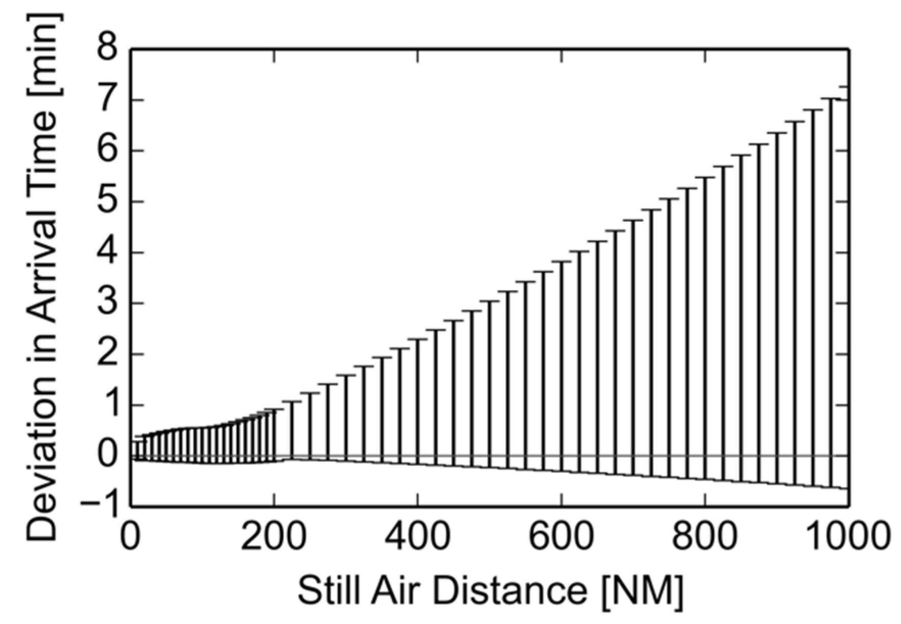
The ATU is the most significant uncertainty for ATM applications [8], since it defines the ability to arrive at an ATM-relevant reference point within a defined timeframe. In this case study, however, the method is exemplified on the VTU during climb phase, where large uncertainties have been identified. Furthermore, a long-term forecast of the ATU shows the expected accuracy in TP using the applied method.

The VTU characterizes the deviation in altitude at a certain point in the 4D trajectory. Since the actual climb performance of an aircraft is sensitive to flight performance parameters, the VTU is widely prominent during climb and descent. The XTU is defined as the lateral deviation from the desired flight track, an issue widely addressed by the RNP concept introduced in the PBN Manual [12]. However, the XTU is not affected by those uncertainties analyzed in this study.

1.3. Interferences as Sources of Position Uncertainty

Position uncertainties are the result of various interferences with different causes and a particular impact on the 4D trajectory. For interferences, which are clearly distinguishable and enable a definite causal link between cause and effect, so-called cause-and-effect models can be developed to include the interference in the TP. The approach has been already applied to trajectory uncertainties [14]. From the perspective of TP, interferences have been categorized similarly, e.g., by Mondoloni [11] or Casado et al. [15]. When further abstracted to an operative perspective, interference as cause of the uncertainties may be distinguished between external (e.g., atmospheric and ATM-related) and internal (e.g., human factors, technical and flight performance).

External interferences directly affect the aircraft’s track. Therefore, the uncertainty in the georeferenced position depends on interference, which directly disturbs the Ground Speed (GS).

Internal interferences, however, originate inside the aircraft itself, so the impact to the 4D trajectory arises indirectly from the airframe through aerodynamics, i.e., resulting in a deviation in the True Air Speed (TAS). Moreover, technical systems, like the autopilot or the flight management system (FMS) may reduce or increase the aircraft position uncertainty. Furthermore, the exact flight control logic is often unknown to TP applications, so higher-level modelling errors for internal interferences are expected.

Additionally, external and internal interferences are distinguished between pre-flight interferences (uncertainties in the aircraft state before departure, so-called initial conditions in [11,15]) and in-flight interferences (dynamic uncertainties throughout phases of the flight).

The behavior of uncertainties in flight dynamics can be handled in different ways, depending on the characteristics of the uncertainties. Especially for external interferences, an analytical conversion of the input PDF to the output PDFs is often possible. An example for this approach is the conversion of uncertainties in the headwind component to the resulting ATU [16,17]. Considering a set of random input variables, a straightforward way to handle the problem analytically is the transformation of the stochastic behavior of the input variables into a probability density function of the output variables, e.g., by using a bivariate transformation [18]. However, this approach is only possible for a restricted number of independent uncertain variables. If the input variables are described by a PDF, the Polynomial Chaos method can be applied to calculate mean values and standard deviations of the output variables [6,19]. Both approaches assume independent stochastic input variables. This assumption only covers a part of the identified uncertainties. Considering optimized trajectories, the desired speeds and altitudes depend on ATOM (determining the gross mass), fuel flow and atmospheric conditions, which in turn are burdened with uncertainties themselves. From this, a non-linear optimization problem follows, which cannot be solved analytically. In this study, a method for TP with uncertain ATOM (inducing uncertainties in speeds and altitudes) is presented, which includes uncertain weather conditions.

1.4. Uncertainties in the Actual Take-Off Mass

A central input variable for flight performance calculation and therefore an important internal interference is the actual gross mass of the aircraft [6,9]. According to the previously described categorization, the actual gross mass can be divided into pre-flight interference Actual Take-Off Mass (ATOM) and in-flight interference mass reduction due to fuel burn.

According to ICAO Doc. 4444 PANS-ATM, the ATOM is currently not included in the ATC flight plan [20]. Therefore, the ATOM remains unknown to the ground-based TP. As discussed by Šošovička et al. [21], the actual gross mass, among other FMS-based data, may be communicated via Automatic Dependent Surveillance-Contract Extended Projected Profile (ADS-C EPP) reports in the future. This would increase precision in the actual gross mass for TP applications; some uncertainties will however remain, since weighting is not required for all types of luggage or passengers according to the legal requirements for flight planning.

Additionally, the accuracy of the flight performance model significantly influences the assessment and therewith the impact of ATOM uncertainty on the TP, e.g., fuel burn, flight path, climb and descent angle. For this reason, the flight performance model COALA [8] has been used in this study to provide reliable input for aircraft-related behavior.

1.5. Prediction of the Climb Phase and Top of Climb Locations

TBO enables continuous climb operations (CCO) with significant efficiency-raising potential [22,23]. Optimum CCOs strongly depend on aircraft type-specific aerodynamics (particularly aircraft mass, drag polar as well as speed and altitude intents) and atmospheric parameters (such as wind conditions, pressure- and temperature gradients) [22]. Therefore, CCO is a suitable flight phase for the estimation of those flight-specific variables for TP. Specifically, the current aircraft position as well as the location and time of the Top of Climb (TOC) are related to the aircraft mass, desired cruising altitude and speeds, and the airline intentions on Cost Index (CI).

The usage of a data pool (ADS-B data) of different aircraft types and gross masses at a single airport to predict the current climb phase of a reference flight has been already applied in [24,25,26] with a LAT of five minutes. Here, the flight performance language AIDL (aircraft intent description language) [27] is used to model aircraft performance, which is restricted to constant speeds and climb rates per flight segment. We enhance this method to the whole flight, considering several uncertainties (gross mass, non-constant speeds and altitudes) by using a reliable flight performance model with real weather conditions, considering uncertainties in wind direction and wind speed. The data pool for the TP is generated by a Monte Carlo simulation under conditions of the International Standard Atmosphere (ISA).

2. Cause-And-Effect

The impact of several interferences on the aircraft position uncertainty is estimated by a cause-and-effect model that can be applied to any type of interference, if this interference can be represented by an uncertainty source using a continuous PDF. Therefore, the cause-and-effect model transforms the PDF of the interference into an aircraft position uncertainty before the actual flight event. The aircraft position uncertainty itself is represented by up to three output PDFs, describing the behavior of ATU, VTU, and XTU depending on the Look-Ahead Time (LAT).

$$f_{\mathrm{input}}\left(\mathrm{x},t\right)\to \left[\begin{array}{c}ATU\left(x,t\right)\\ VTU\left(x,t\right)\\ XTU\left(\mathrm{x},t\right)\end{array}\right]$$

(1)

As shown in Equation (1), the input PDF $f_{\mathrm{input}}$ also depends on the LAT. For pre-flight interference, i.e., error in the initial state, the input PDF simplifies to $f_{\mathrm{input}}\left(x\right)$.

By using this cause-and-effect model, multiple interferences can be merged to one overall position uncertainty by a convolution of probability distributions as long as the resulting position uncertainties are probabilistically independent. Furthermore, the final cause-and-effect model is analytically solvable, since all computationally expensive calculations have been done before the actual flight, thus increasing its efficiency. The general principle of a cause-and-effect model is illustrated in Figure 2.

In this study, the ATOM is assumed as unknown, thus a cause-and-effect model for an internal interference with an uncertain pre-flight state is developed. Therefore, the impact of the ATOM to the movement relative to the air mass in form of an uncertainty in the resulting TAS needs to be analyzed first.

Afterwards, the resulting uncertainty in the TAS is converted to a GS considering uncertain weather scenarios. The following two steps are applied on assuming an uncertain ATOM (compare Figure 3).

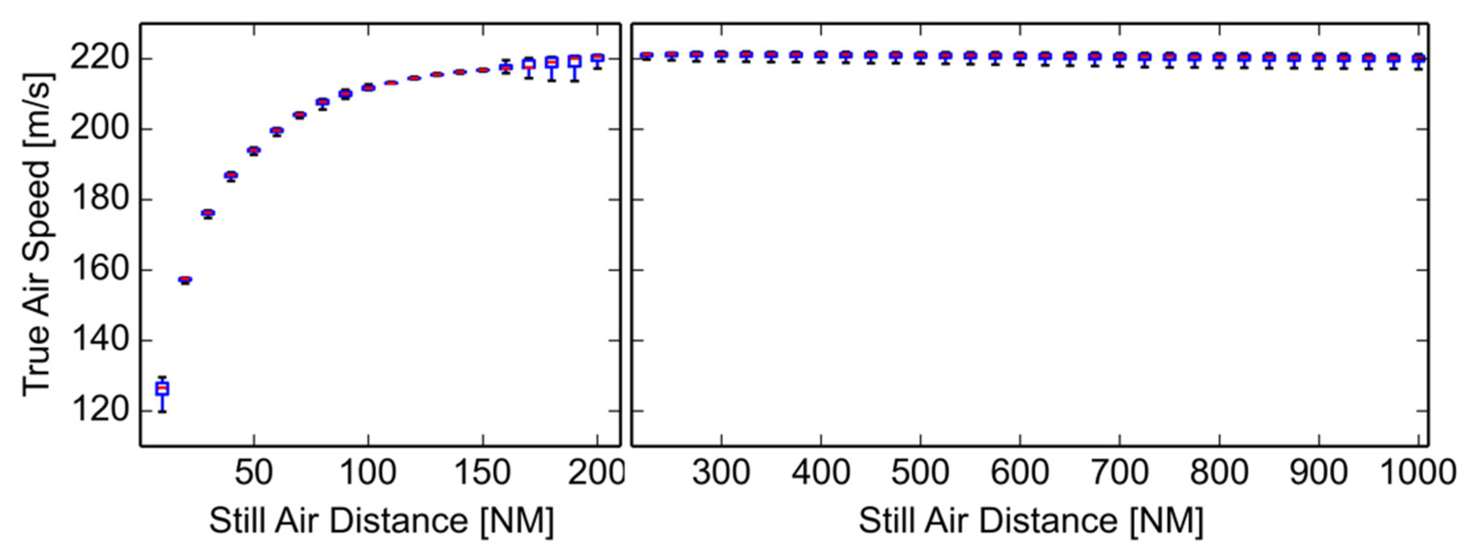
In the pre-flight uncertainty impact assessment, all other factors that may contribute to a probabilistically dependent position uncertainty are excluded to quantify the impact of the ATOM on ATU and VTU elaborately. Therefore, a Monte Carlo simulation with stochastically distributed ATOM is established and analyzed regarding observed differences in ATU and VTU. To ensure a high statistic reliability, 11,000 simulation runs are proceeded. Although the true air speed is non-constant and optimized in each simulation run, the convergence of the results to a constant value is ensured more than 8000 simulation runs (Figure 3). ATU and VTU are additionally burdened with uncertainties of the TAS, because the TAS is used as optimization target function in the flight performance model. Other related uncertainties, such as an uncertain mass change over flight time, are neglected. In this state, weather interferences are also excluded; thus, all calculations are conducted in an ISA atmosphere with zero wind.

The in-flight uncertainty calibration provides a method to predict future aircraft positions by applying the previously generated results of the cause-and-effect model (i.e., the observed ATU and VTU distributions of the Monte Carlo simulation) to real-weather scenarios. Here, the weather interferences are added to demonstrate the application in the TP algorithm, while a demanding Monte Carlo simulation run is no longer required in real weather conditions.

For application of the cause-and-effect model, further assumptions are made: To avoid ATOM-specific instabilities in the first climb segment (i.e., differences in take-off distance), e.g., interferences due to aerodrome conditions (obstacles, runway conditions) and operator procedures (thrust rating, safety margins, preferred climb-out procedure), the analysis starts at approximately flight level (FL) 100, i.e., 10,000 ft altitude. During climb, the trajectories are sliced every 10 NM, where values for ATU and VTU are calculated. During cruise, the trajectories are sliced every 25 NM, where ATU value is calculated; the VTU can be excluded since a static cruising altitude is assumed. The location of the TOC (still air distance from take-off) and the time until TOC are also analyzed, since the TOC characterizes the transition between phases of the two flights. In this study, the Top of Decent and the descent phase are excluded for reasons, which are limited by the modelling process [28]. Furthermore, XTU is not analyzed, because no significant impact of ATOM on XTU is expected. The impact of uncertainties in weather on XTU is compensated by the FMS, since PBN procedures [12] already require the aircraft to remain within the RNP boundaries of the airway in today’s ATM system.

2.1. Pre-flight Uncertainty Impact Assessment

The pre-flight uncertainty impact assessment quantifies the impact of the interference, characterized by the input PDF, to the aircraft position uncertainty. It is assumed that the aircraft has fairly accurate knowledge regarding the most significant interference on aircraft position accuracy, while the TP application on the ground remains unaware of this knowledge. This assumption is acceptable due to the FMS feedback control laws, which react based on the actual aircraft behavior. Thereby, the aircraft is requested to select its preferred speed based on the current aircraft state instead of a fixed speed assumed in comparable research [6,9,19]. The freedom to select the speed will increase the impact of internal interferences significantly. However, a free choice of speed is a prerequisite for a TBO environment, so that the ecologic and economic goals of SESAR can be reached [1].

Based on this assumption, a numerical conversion is ruled out, since the optimized speeds need to be calculated continuously. Because the uncertain gross mass causes uncertainties in the selected speed, the established Polynomial Chaos method cannot be applied. Therefore, a Monte Carlo simulation is applied. Here, 11,000 complete trajectories are calculated utilizing the same aircraft type Airbus A320 [29].

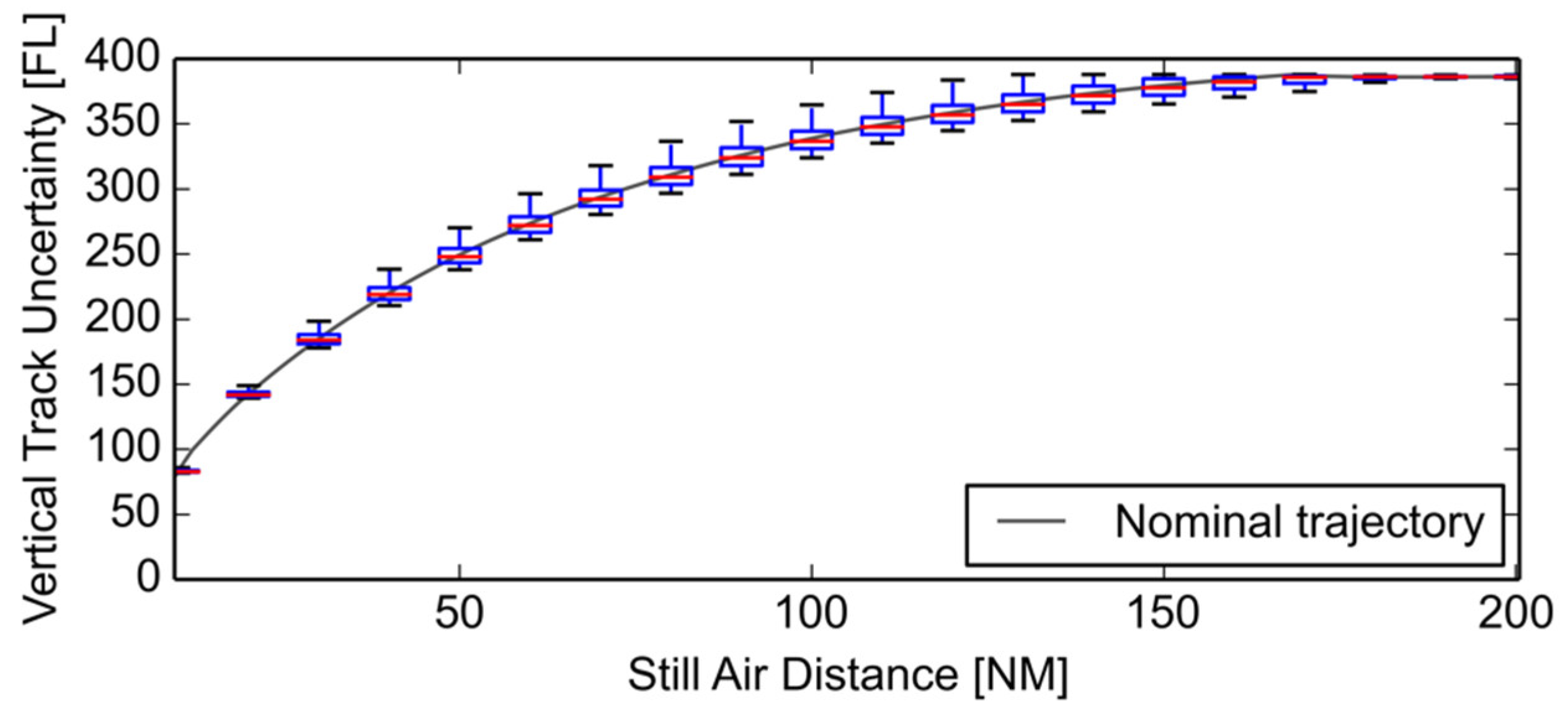
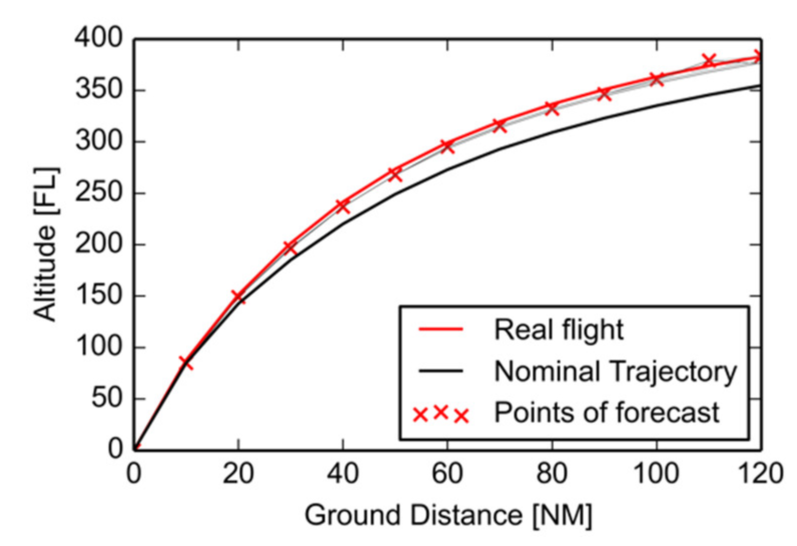
To characterize the impact of the interference clearly, a nominal trajectory is generated using the expected value $E\left(X\right)=ATOM$ of the input ATOM PDF (compare Figure 4).

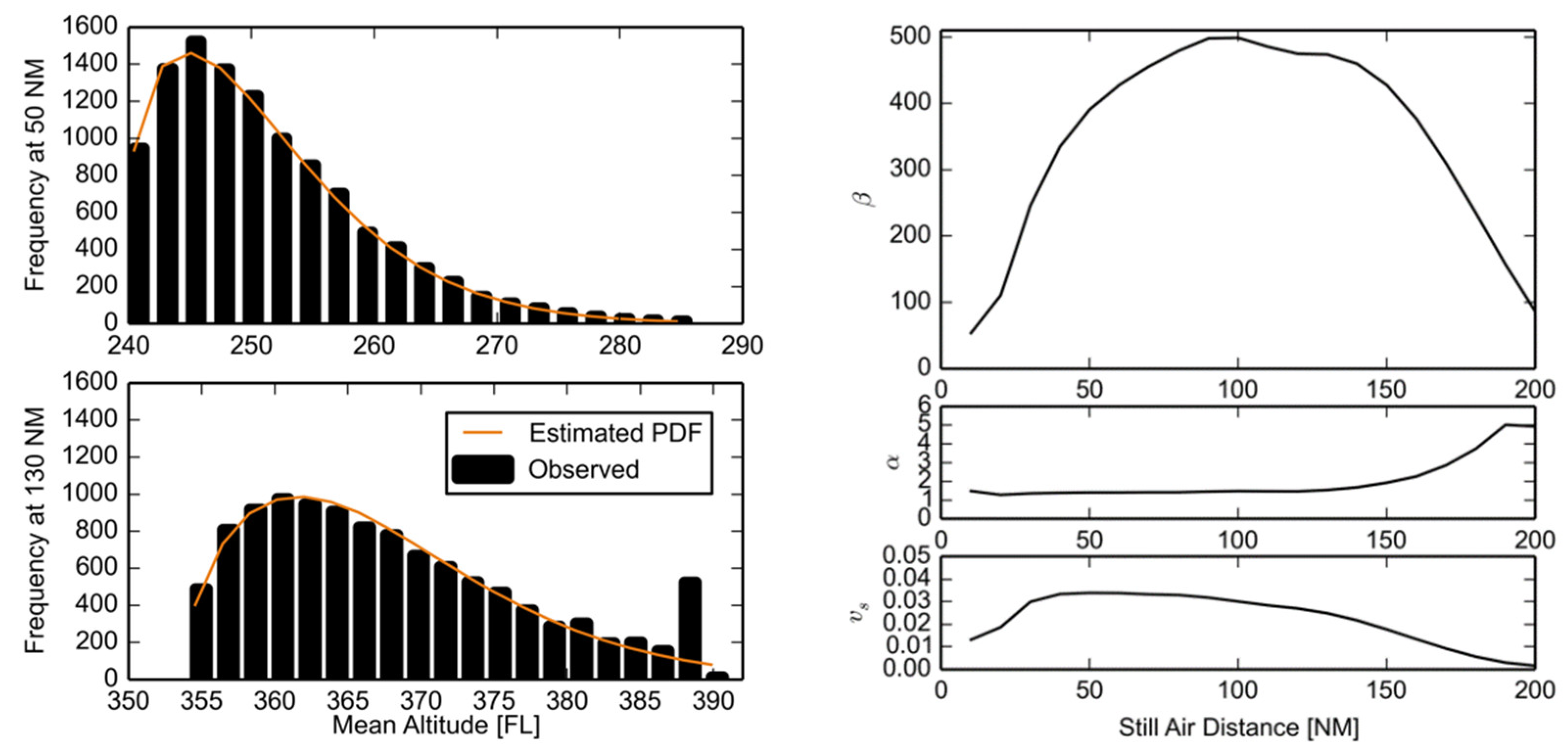
For the impact assessment, points of interest are defined along the trajectory at fixed still air distances (slices), measured from the take-off location. At each slice for each flight, the along-track error ATE [s] and vertical-track error VTE [ft] are calculated with reference to the nominal trajectory. Based on the errors observed for all flights, the parameters of the ATU and VTU distributions can be determined through classification and parameter estimation with a goodness-of-fit test (Pearson Chi-square test) assuming a Weibull distribution (with parameter α and β for shape and scale, respectively). Furthermore, a regression analysis of the distribution parameters provides information concerning the propagation over the LAT.

2.2. In-flight Uncertainty Calibration

If the relation between the input PDF and output PDF is established and proven, ATU and VTU can be handled deterministically without additional Monte Carlo simulations. Therefore, the further path of a flight with a random ATOM following the previously parametrized PDF, e.g., $X\left(x;\alpha ,\beta \right)$, will be predicted. Therewith, the actual ATOM is considered as unknown to ATM and its TP applications, but the proven relation between input PDF (of ATOM) and output PDF (of ATU and VTU), derived from the pre-flight uncertainty impact assessment (i.e., the Monte Carlo Simulation under ISA conditions), is applied.

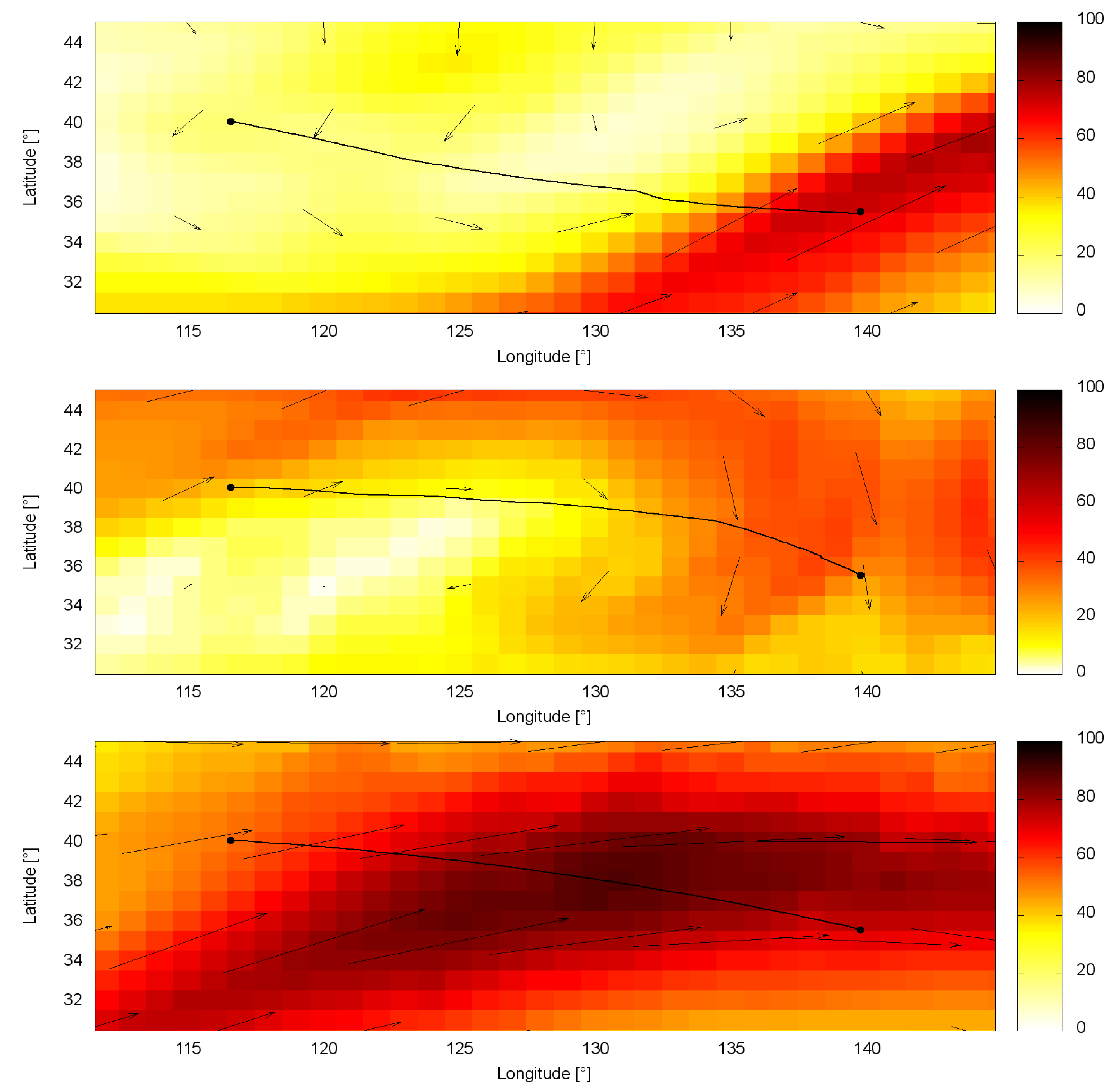
As a starting value at $k=1$, the expected value $E\left(X\right)$ of the input PDF is used to compute the initial predicted trajectory $T_{E\left(x\right),k=1}$ in the real weather taken from the Global Forecast System (GFS) [30], provided by the National Oceanic Atmospheric Administration. The weather data sets are chosen according to significant differences between each other (compare Section 3.2). The GFS weather data used for the calculation of the real flight trajectory, however, is additionally burdened with normal distributed uncertainties in both wind components of ${\sigma }_u={\sigma }_v=5$ m/s. Details of this procedure are described in [28]. As soon as the real flight reaches the first slice (i.e., 10 NM still air distance), the initial predicted trajectory $T_{E\left(x\right),k=1}$ is compared with the observed real trajectory $T_{X,k}$ by calculating the errors $AT{E}_{k,Weather}$ and $VT{E}_{k,Weather}$ in real and uncertain weather conditions with unknown ATOM (Figure 4).

At each slice, $AT{E}_{k,Weather}$ and $VT{E}_{k,Weather}$ between the previously predicted trajectory $T_{E\left(x\right),k}$ and the real flight $T_{X,k}$ are estimated. Assuming that relative values of $AT{E}_{k,Weather}$ and $VT{E}_{k,Weather}$ are equal to those relative values in ISA, we transform them in absolute values in ISA and determine a new estimated $ATOM (AT{U}_{k,Weather}$, $VT{U}_{k,Weather}$) using the derived relationship between input PDF of the mass and output PDFs $AT{U}_{k,ISA}$ and $VT{U}_{k,ISA}$. Based on the updated $ATOM (AT{U}_{k,Weather}$, $VT{U}_{k,Weather}$) estimation, a new predicted trajectory $T_{E\left(x\right),k}$. is calculated with the GFS weather forecast. In the same procedure, $AT{U}_{k+1,Weather}$ and $VT{U}_{k+1,Weather}$ between $T_{E\left(x\right),k+1}$ and $T_{X,k}$ at the next slice $k+1$ are used to incrementally adjust ATOM to the unknown value of $T_{X,k}$. The procedure is illustrated in Figure 4.

2.3. Modelling of the ATOM Uncertainty

For impact assessment, the following assumptions are made: The aircraft type is set to an Airbus A320-212 with CFM56-5A3 engines, with static Operating Empty Mass $OEM=39,000\mathrm{kg}$ [29]. The trip fuel is set to $m_{\mathrm{f}}=7,000\mathrm{kg}$. The payload varies following a Weibull-distribution.

$$f\left(x;\alpha ,\beta \right)=\{\begin{array}{rr}\frac{\alpha }{{\beta }^{\alpha }}{\mathrm{x}}^{\alpha -1}{e}^{-{\left(x/\mathsf{\beta }\right)}^{\alpha }},& x\ge 0\\ 0,& x<0\end{array}$$

(2)

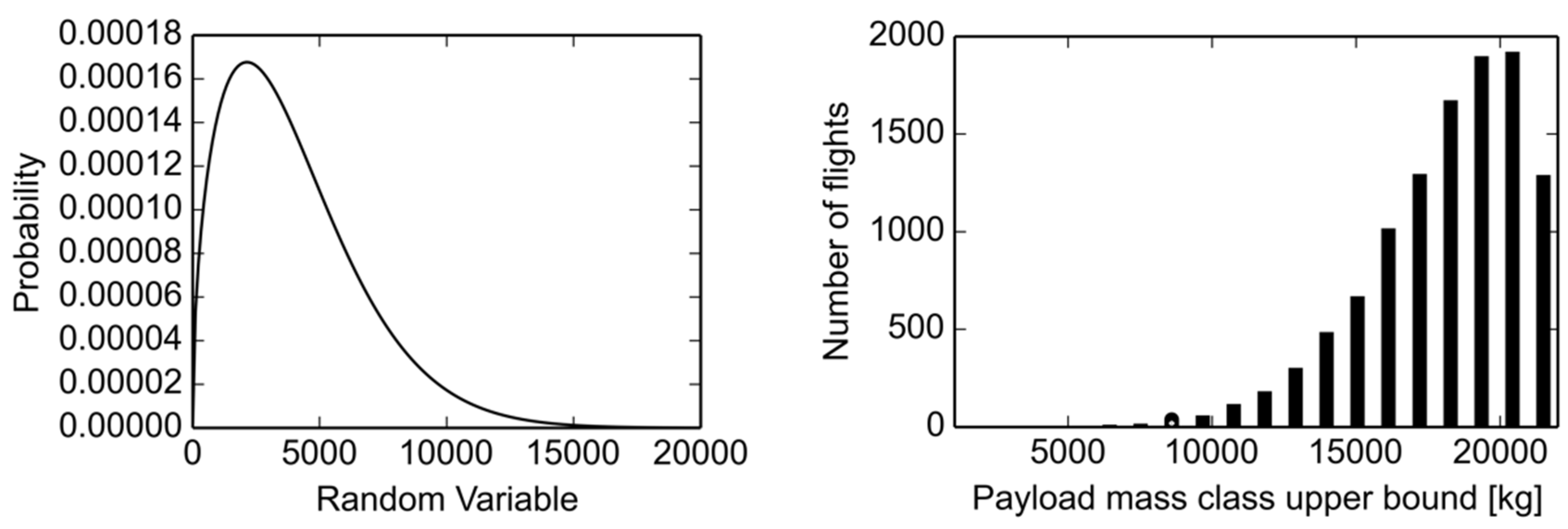
As shown in Equation (2) and Figure 5 left, the advantage of the Weibull-distribution is that it is zero for x < 0. This characteristic of the PDF is used to ensure that the payload never exceeds the maximum permitted payload of $m_{\mathrm{p},\max }=21,500\mathrm{kg}$ [29]. Furthermore, the expected value for the payload should be close to the maximum permitted payload. To cope with these requirements, the shape parameter is set to $\alpha =1.5$, while the scale parameter is set to $\beta =4444$, resulting in a positive skew with a sharp incline in the beginning and a smooth reduction after the mode. To meet the proposed assumptions, the resulting random numbers $X_{\mathrm{i}}$ are mirrored, leading to an ATOM for each flight $i$ calculated as:

$$ATO{M}_{\mathrm{i}}=OEM+m_{\mathrm{f}}+m_{\mathrm{p},\max }-X_{\mathrm{i}}$$

(3)

with the Weibull-distributed unused payload $X_{\mathrm{i}}$ [kg]. With this approach, the probability for a payload above the maximum permitted payload is $p_{m_{\mathrm{p}}>m_{\mathrm{p},\max }}=0$, while the probability for a payload below zero remains low ($p_{m_{\mathrm{p}}<0}=0.00002$, compare Figure 4).

For the calculation of the nominal trajectory, the expected value E(X) of the Weibull distribution is determined by:

$$E\left(X;\alpha ,\beta \right)=\beta ·\mathsf{\Gamma }\left(1+{\alpha }^{-1}\right)$$

(4)

utilizing the Gamma function $\mathsf{\Gamma }$, which yields $E\left(X\right)=4,011.8$ kg. With Equation (3), the ATOM for the nominal trajectory is set to $ATO{M}_{\mathrm{nominal}}=63,488.2\mathrm{kg}$.

Note, these assumptions are chosen solely to demonstrate and validate the methodology, which is adaptable to any kind of PDF.

For the analysis of the Monte Carlo simulation, the Weibull parameters β and α of the observation sample have been estimated following Gumbel’s [31] procedure:

$$\alpha =\frac{1.25}{v_s}-0.45\mathrm{for}{v}_s\le 0.4651\mathrm{and}$$

(5)

$$\beta =\frac{\overline{x}}{\mathsf{\Gamma }\left(1+\frac{1}{\alpha }\right)}$$

(6)

where $\mathsf{\Gamma }$ and $\overline{x}$ denote the Gamma function and the mean of the observed data, respectively. For the Chi-squared test of goodness of fit, the observed values have been classified according to Sachs [32] in $k$ classes with $k=5\log n=20$, where $n=11,000$ denotes the total number of observations. 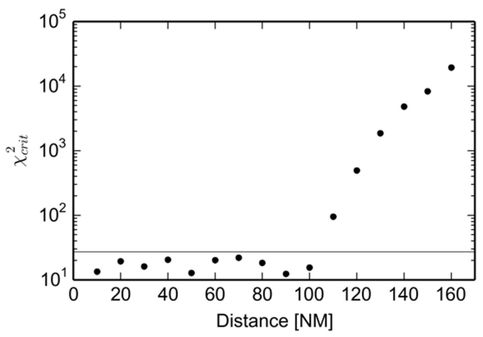Following [33], $k=20$ is near to the maximum number of classes for Pearson’s Chi-squared test of goodness of fit [34]. The critical value ${\chi }_{crit}^2$ is derived from the inversion of the Chi-squared distribution density function:

$$f\left({\chi }_{crit}^2,\lambda \right)=\frac{x^{\frac{\lambda }{2}-1}{e}^{-\frac{x}{2}}}{2^{\frac{\lambda }{2}}\mathsf{\Gamma }\left(\frac{\lambda }{2}\right)},$$

(7)

where $f\left({\chi }_{crit}^2,\lambda \right)$ estimates the significance level $a$ (which is set to $a=0.05$) and $f\left({\chi }_{crit}^2,\lambda \right)$ depends on the degrees of freedom $\lambda =k-m-1=17$, where $m$ denotes the number of parameters, which is in case of the Weibull distribution. The critical value ${\chi }_{crit}^2$ is compared with the test statistic ${\chi }^2$

$${\chi }^2={{\displaystyle \sum }}_{i=1}^k\frac{{(x_i-m_i)}^2}{m_i}.$$

(8)

Here, $x_i$ describes the observed numbers per class and $m_i$ denotes the expected numbers per class, derived from the probabilities of the sample distribution (i.e., the Weibull distribution). In case of ${\chi }^2\le {\chi }_{crit}^2$, the hypothesis, announcing that the observed values are describable by the sample distribution, does not have to be declined.

2.4. Simulation Environment

The trajectories of the Monte Carlo data pool are calculated with the flight performance model COALA, which allows the prediction (4D position, speed, fuel flow, acting forces) along the flight path. COALA is a point mass model, respecting all acting forces (including acceleration forces) and aircraft type-specific performance envelopes. In order to do so, COALA generates only physically feasible trajectories. Optimized speeds, flight path angles, and cruising altitudes are calculated as target functions and the lift coefficient is used as controlled variable in a proportional–integral–derivative controller. In the current study, the following state variable selection paradigm is assumed [8]: A continuous climb is conducted, first with maximum angle of climb below FL 100, then with maximum climb rate until top of climb (TOC). In the cruise phase, speed and altitude are selected based on the maximum specific range $R_{\mathrm{spec}}=TAS/{\dot{m}}_{\mathrm{f}}$, i.e., with the optimum gain in TAS per unit rate of fuel flow ${\dot{m}}_f$. Continuous descent operations are performed with speeds and descent angles for a maximum lift ($F_L$) to drag ($F_D$) ratio $E=F_L/F_D$.

3. Assessment of Uncertainties

3.1. Assessment of Observed Uncertainties

In the Monte Carlo Simulation, trajectories between Beijing Capital (ZBAA) and Tokyo Haneda (RJTT) with a ground distance of d $\approx 1,120$ NM are generated. For the first trial, the cruising pressure altitude has been defined to $p_{cruise}=200$ hPa. The target TAS during climb nonlinearly depends on ATOM (Figure 5, left). After significant differences in Lift-Off speed ($\Delta TAS=12$ m/s) similar shares of energy are investigated in kinetic energy during ascent. Differences increase again (up to $\Delta TAS=8$ m/s); as soon as light aircraft are already in cruise and heavy ones are still in the climb phase. During cruise, differences in TAS ($\Delta TAS\approx$ 10 m/s) are increasing slightly due to the relative share of mass loss due to fuel consumption (Figure 6, right). The analytical target function for a speed with a maximum specific range gains in higher optimum speeds for heavier aircraft.

Figure 7, Figure 8, Figure 9 and Figure 10 give evidence that Weibull-distributed uncertainties in the ATOM induce a Weibull-distributed VTU, since the observed means (red) in VTU exactly represent the nominal trajectory (grey). Furthermore, the shapes of the classified observed altitudes until 100 NM, e.g., as shown in Figure 8 for 50 NM still air distance, clearly indicate a correct sample distribution. Beyond 100 NM, however, the Chi-squared test for the goodness of fit of the Weibull distribution fails due to a small coefficient of variation $v_s$ (compare also Figure 9). The bottom left histogram in Figure 8 for 130 NM reveals another reason for the failure of the test; with an increasing number of aircraft already in the cruise phase of the flight, the characteristic of the Weibull distribution slowly fades. This effect is also visible in Figure 6, where the solution space for the observed TAS extends significantly between 100 NM and 200 NM. Therefore, the VTU can be used for in-flight uncertainty calibration as long as all aircraft remain in the climb phase.

Further details on the estimated Weibull parameters and the results of all goodness of fit tests for each uncertainty at each slice may be requested from the authors.

The uncertainty in arrival time at certain slices of ground distance shows the expected nonlinear behavior with relatively small values of ATU in the climb phase and increasing differences in cruise. The strong correlation of this estimation with the analysis of TAS (Figure 6 and Figure 10) suggests a distinct relationship between uncertainties in ATOM and ATU. Hence, those uncertainties can be efficiently reduced with in-flight uncertainty calibration, as proposed in the study.

3.2. Assessment of the In-flight Uncertainty Calibration

The proven relationship between input PDF and output ATU and VTU is now used to predict the trajectory with unknown ATOM and unknown non-constant TAS in uncertain weather conditions. The method has been tested on three different weather scenarios from (A): 25^th July 2016; (B): 17^th May 2017 and (C): 29^th November 2017. The dates are chosen according to significant differences in wind speed and wind direction, resulting in differences in ground distance to the TOC up to 60 NM (compare

Table 1. Comparison of the observed ground distances to the Top of climb (TOC) for different weather scenarios and the ISA scenario without wind.

Weather	Observed Ground Distance to TOC [NM]
	Nominal	20,000 kg 1	15,000 kg 1	10,000 kg 1
ISA	168.3	195.8	149.1	121.1
A	213.2	247.8	186.7	152.3
B	148.6	174.2	128.2	106.8
C	209.0	245.7	183.0	149.4

¹ Payload is used to calculate the Actual Take-off mass (ATOM).

). The impact of these weather scenarios on trajectory optimization are shown in Figure 11. The weather data are provided by the National Oceanic and Atmospheric Administration and are used for $T_{\mathrm{Forecast}}\left(ATOM \left(VT{U}_{k+1}\right)\right)$ as available weather data set for trajectory prediction.

To consider the uncertainty in weather forecast with impact on the trajectory acting as the real flight $T_{\mathrm{Real}}\left(X\left(x;\alpha ,\beta \right)\right)$, both wind components are burdened with normal distributed uncertainties with a standard deviation of ${\sigma }_{u,v}=5$ m/s. The TP application, however, remains unaware of the altered weather situation and continues to predict based on the original weather forecast, even when position updates of the real flight trajectory $T_{\mathrm{Real}}\left(X\left(x;\alpha ,\beta \right)\right)$ are available. Hence, the vertical error as a measure to adjust the ATOM is influenced by ATOM and by differences in weather between ISA (no wind), Forecast (µ) and Real~N(µ,${\sigma }_{u,v}$). The developed methodology could be successfully applied to all weather scenarios and to trajectories with three different unknown ATOMs (compare Figure 12 and Figure 13).

Starting 10 NM after take-off, differences in VTU are expected to be small. Nevertheless, the algorithm is able to adjust the ATOM (initially the expected value, represented as “Nominal Trajectory” in Figure 12) efficiently to the real ATOM.

Therewith, the position of the TOC could be predicted in all scenarios. To avoid fluctuations due to real weather data, a threshold of 0.5% in the relative vertical error was implemented to decide on adjusting ATOM in the current iteration loop (i.e., at the current slice) or not. Based on this, the relative vertical errors in the trajectories with 20,000 kg payload remained unchanged in every weather scenario (Figure 13).

4. Conclusions

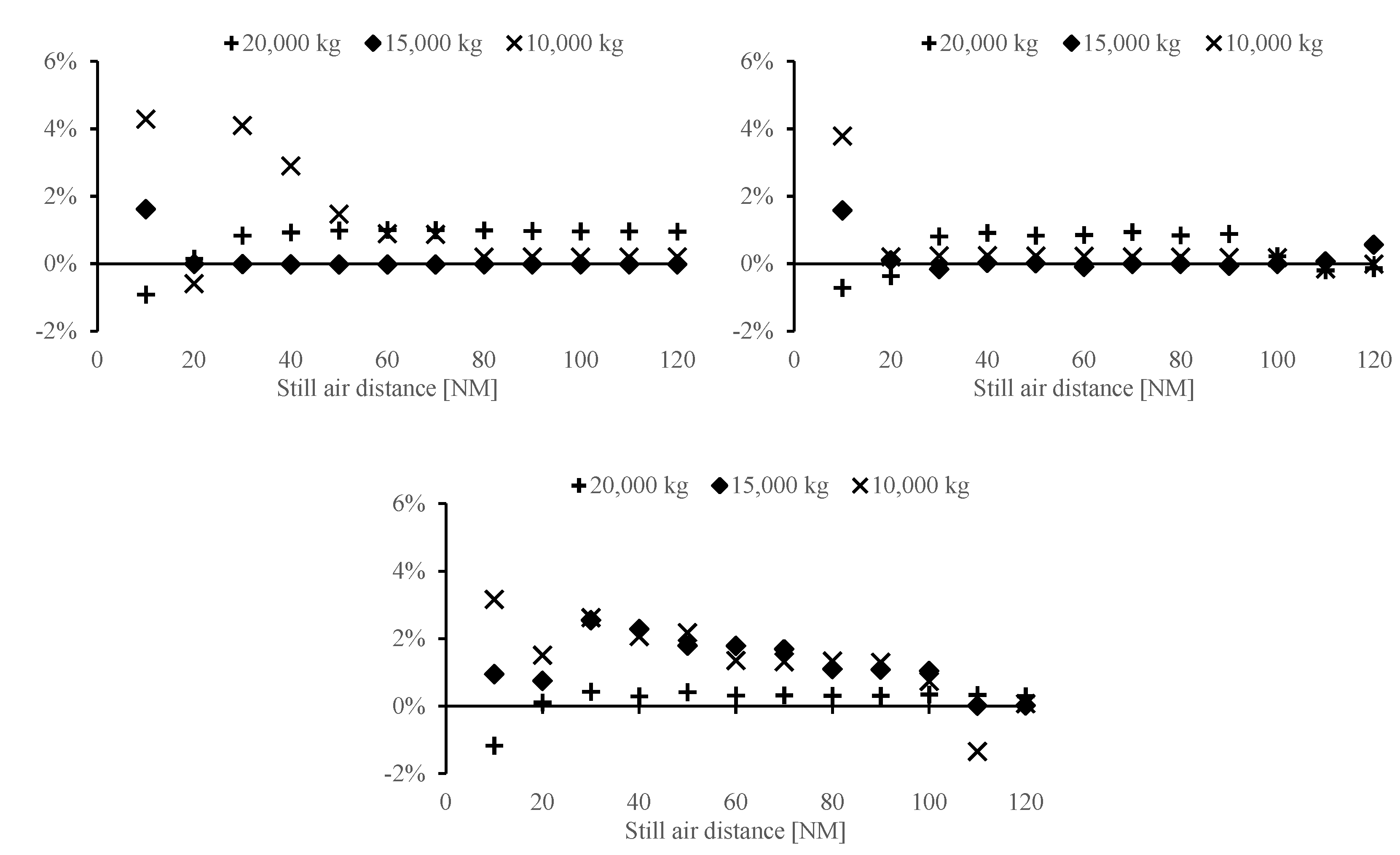
In this case study, a methodology was developed and validated to transform an arbitrary probability density function (PDF) defining a source of uncertainties into a PDF of vertical errors and along track errors, thus describing a 4D aircraft position uncertainty. The numerical transformation of the input PDF to the output PDF has been exemplified along a Weibull-distributed Actual Take-Off Mass with impact on the optimization function for TAS. Thereby, the focus explicitly laid on non-linearly dependent uncertainties (ATOM, TAS), which have been combined with non-classifiable uncertainties, such as real weather conditions with further impact on TAS. The approach has been tested for the TP of the climb phase with significant values of VTU. The method has been applied to three interdependent uncertainties (ATOM, TAS and uncertainties in weather prediction) under three significantly different weather conditions. In each scenario, the in-flight uncertainty calibration has succeeded in five iterations.

In the same way, the algorithm can be applied to the cruise and descent phase, which is of minor scientific interest due to small-expected uncertainties, as far as the speed strategy of the aircraft is known, even different cruising altitudes or continuous cruise climb procedures are easily to detect in the first minutes of the cruise phase.

The approach may be applied to any kind of uncertainty, which is phrase-able as probability density function. In the case of multiple uncertainties, the resultant PDF may be estimated either by a stochastic variation of all uncertainties or, if possible, by identifying most significant relations between uncertainties and interferences. A successful implementation of the developed approach requires the identification of those interferences (e.g., ATU, VTU), which are most affected by the uncertainty (e.g., ATOM, TAS, wind) in question. This can be done by a principle component analysis.

In the future, the approach will be applied to more complex uncertainties. Uncertainties in the cost index as an unknown parameter influencing fuel flow ${\dot{m}}_f$ and ground speed GS by controlling the TAS will be investigated. Furthermore, uncertainties in the fuel flow ${\dot{m}}_f$ (i.e., an uncertain change of mass during flight) will be discussed. The results will be compared with a different approach, developed by Casado et al. [9].