1. Introduction
The fluid-structure interactions (FSI) study is one of the most important steps in the design procedure of deformable flying objects. These interactions could be stable or oscillatory. In oscillatory interactions, the strain that is induced in the solid structure causes it to move, such that the source of strain is reduced, and the structure returns to its former state only for the process to repeat. The aeroelastic problems did not occur if aircraft structures were rigid. However, modern aircraft structures are flexible with respect to weight considerations. Aeroelastic instabilities involve aerodynamic forces that are generated due to the motion of the structure, and may cause structural deflection. The aerodynamic effects, such as buffeting, refer to the fluctuating nature of the wing (and its interaction with the structure) and sometimes cause aerodynamic instability. When buffeting, flutter instability, and etc. occurred, aerodynamic and aeroelastic effects play a major role in the design of flexible structures [
1]. The aerodynamic and aeroelastic effects will cause nonlinearities in the system that result in different dynamic behaviors, like limit cycle oscillations (LCO), infinite increase in the amplitude, and chaotic behavior. Therefore, the study of these effects plays a vital role in the design and analysis of the flying objects. The effect of laminate lay-up on flutter speed of composite missile stabilizers for the subsonic flight conditions is comprehensively investigated in [
2] based on a two-dimensional (2D) flutter model. The authors have used a finite element approach based on the Lanczos method to achieve optimum results in respect to solution accuracy and computational cost.
One of the main limitations of the linearity assumption is the inability to predict the system behavior after starting the instability. In reality, some kind of nonlinearities may prevent the amplitudes from going to infinity. In nonlinear systems, vibration with limited amplitude or chaotic motion occurs in upper or lower of the flutter speed—the speed that the response of domain does not change with time [
3]. Despite the fact that these two types of motions do not lead to destructive failure in structures, these can lead to fatigue failure or destructive effect on control systems. Therefore, the effect of nonlinear phenomena on aerodynamics behavior should be considered in the design process of flying objects.
Generally, the instability in aero-elastic systems can be traced from aerodynamic or structure sources. The nonlinear terms of aerodynamic can be the effects of shock motion, high angle of attack, flow separation, transonic flow, to name but a few. Besides, the nonlinear terms of structures can be inclusive of freeplay between components or control systems, large deformations, material nonlinearity, the effects of friction in control cables or bearings, the limitations in kinetic energy of control surfaces, and concentrated non-linear terms that may be related to elastic deformation in connections.
Kholodar explained why a certain amount of the preload or angle of attack could be the main reason for the unexpected higher-frequency oscillations. This study shows that a certain preload is required to excite limit cycle oscillations [
4]. Marsden and Price have done an experimental analysis to show that, when freeplay nonlinearity is introduced in the pitch degree of freedom, the flutter speed that is estimated by extrapolation of the damping curve decreases with increasing the freeplay size [
5]. A free vibration analysis is performed while using the finite element, and the fictitious mass methods in [
6] in which aero-elastic responses included LCO, unstable LCO, and periodic motion are observed for air speeds below the linear flutter boundary. Moosazadeh, et al. assumed a fully nonlinear structure with nonlinear third order piston theory to show that the stability increases with freeplay in high speed and increasing the velocity will decrease the damping effect in post flutter behavior [
7]. The challenges and characteristics of the flow past the body at critical angles of attack based on modern aerodynamics explained in [
8]. The author showed that the separation starts from the trailing edge and moves towards the leading edge, proportionally to the increase of the angle of attack, although critical angles of attack depends on the type of the airfoil, the local characteristics for the defined conditions of the flow, and the dynamics of the angle of attack. The best actual lift-curve slope of the conventional symmetrical NACA 0012 airfoil according to the Mach and Reynolds flow numbers is obtained in [
9]. Rasuo analyzed the principal factors that influence the accuracy of two-dimensional wind tunnel test results [
10], and the influences of Reynolds number and Mach number on two-dimensional wind-tunnel testing [
11]. Ocokoljić, et al. investigated the requirements for the accuracy of measurements in a wind tunnel, such as calibration of the wind tunnel test section [
12]. Other relevant studies have also focused on stall-induced vibration analysis [
13,
14], bifurcation and chaos analysis [
15,
16,
17], non-linear dynamics [
18], and stability analysis [
19]. It could be concluded that one of the main objectives of all studies in this field is to develop a reliable, precise, and fast method for aero-elastic behavior, stability, and the flutter speed analysis while avoiding numerical integration issues of instability and inaccuracy.
Table 1 lists the main milestones in this field with their advantages and disadvantages.
Gap Analysis
The first step by Theodorsen was limited by this assumption that the harmonic oscillations in inviscid and incompressible flow is subject to small disturbances.
Woolston also just studied a simple aero-elastic system by investigating the effect of freeplay on flutter velocity [
25].
Air Force Wright Aeronautical Laboratories focused on flutter analysis of a NACA 64A006 airfoil (as a case study) pitching and plunging in small-disturbance, un-steady transonic flow.
The steady-state formulations has been used to tackle the indicial lift on a thick-aerofoil response method in the literature. It is practical but still limited.
The method presented by Menon and Mittal is precise and comprehensive (they have used ViCar3D code [
26,
27]) but the huge computational effort is the weakness of this study.
The above analysis confirms the lack of a fast and precise method for predicting and analyzing the effects of freeplay on control surface on the aero-elastic behavior of airfoil. In this paper, a new methodological approach is proposed to predict the aero-elastic behavior, stability, and the flutter speed of an airfoil with very low computational effort and reasonable accuracy in comparison with the published studies. For this purpose, the structural model is developed first while using Lagrange’s equation. Subsequently, using Theodorsen approach, the aerodynamic model is generated. The unstable aerodynamic is also modeled while using Jones approximation. Next, the aero-elastic model is developed by combination of structural and aerodynamic models. After that, the numerical results are generated by numerical integration in state space. Finally, the results analysis, including the flutter speed prediction, stability analysis, sensitivity analysis on freeplay degree, and the effect of freeplay on the time responses are presented and discussed.
2. Equations of Motion and the Proposed Method
For airfoils with high aspect ratio, a two-dimensional modelling approach with equivalent section properly simulates the aero-elastic behavior of 3-D airfoil. The structure is modeled with mass-spring and the aerodynamic is modeled with two dimensional assumptions. Mass-spring structural models have proper accuracy in the most two-dimensional nonlinear structural problems.
The general form of the equations of motion for an elastic system in Laplace domain can be represented, as follows [
28]:
where
is free stream velocity,
is dynamic pressure, and
b is reference length that equal to half of chord of two dimensional airfoil.
,
, and
are mass, damping, and stiffness matrixes, and
is generalized coordinates vector. The
matrix in the generalized aerodynamic forces is defined, as follows:
And
is below dimensionless variable Laplace transform:
where
is equal to
,
is equal to
,
is oscillatory frequency, and
is the rate of decline in transient motion.
There are different methods to obtain eigenvalues of Equation (1) and analyze the instability of system behaviors. In this study, the unsteady aerodynamic and p-method is used because of having more general applications than other method.
Table 2 shows the itemized steps of the proposed method. These steps are described in detail in the next sections.
2.1. Two-Dimensional Structural Modeling of Airfoil
In this paper, the Lagrange’s equations are used in the modeling of structural system. These equations are the form of equations of motion that includes kinetic and potential energy, and have many applications, especially in the analysis of dynamical systems. The general form of Lagrange equation is as follows:
where
is kinetic energy,
is potential energy,
are independent generalized coordinates of system,
are the vectors of generalized forces that include conservative and non-conservative forces, whereas this forces achieved by principle of virtual work, and
n is the number of independent degrees of freedom of the system. The difference between kinetic and potential energy is called the system’s Lagrangian. Kinetic and potential energy parts of the Equation (4) will both be calculated in the next sections.
2.1.1. Kinetic Energy of Two Dimensional Airfoil with Control Surface
First, the coordinate of each point of airfoil is explained to calculate the velocity. According to
Figure 1, the location of each point in the X-Z coordinates system that origin of this coordinate system located in elastic axis is as follows:
Additionally, coordinates of each point of the control surface is calculated, as follows:
By taking the first time derivative of Equation (6), the velocity of each point is obtained, so the kinetic energy of airfoil with control surface given, as follows:
2.1.2. Potential Energy of Two Dimensional Airfoil with Control Surface
According to
Figure 1, based on [
29], the potential energy of airfoil is composed of two parts: The first part is derived from displacement in Z-direction that modeled with spring
, and the second part is torsional potential energy of airfoil that modeled with torsional spring
. Additionally, the potential energy of control surface derived from torsion of control surface about hinge axis that is stored in torsional spring
. Accordingly, the potential energy of airfoil with control surface is calculated, as follows:
2.2. Control Surface Freeplay Modelling
It is assumed that the control surface has freeplay. This eventuates to this assumption that the torsional spring (connection of the control surface to the airfoil) cannot carry forces for some angles of control surface’s displacement. Hence, spring stiffness would be a nonlinear function of angle of torsion. This non-linear behavior is shown in
Figure 2 that approximated into multi-sections.
Hence, restoring moment of control surface
has been shown in (9):
3. The Aerodynamics Model
The aerodynamic forces that are caused by unsteady flow for airfoil are calculated by Theodorsen in [
20]. For airfoil displacement modelling in Z-direction, airfoil torsion, and control surface torsion three springs
,
, and
are used, as shown in
Figure 1. In this model, chord length of airfoil is 2 b and elastic axis located at point that airfoil rotates about it. The center of mass from this airfoil is located at
distance from elastic axis and the hinge axis of control surface is located at
distance from elastic axis. In addition, the center of mass of control surface considered at
distance from hinge axis.
Theodorsen calculated lift
, aerodynamic moment
, and restoring moment
with the assumption of complete oscillatory motion, as follows:
where
ρ is flow density and
is flow velocity. Additionally,
h,
, and
are displacement in Z-direction, airfoil pitch, and pitch degree of control surface. Positive directions of X, Z,
, and
are shown in
Figure 1. The origin of coordinate system XYZ located at elastic axis. The constants
to
that are used in Equations (10)–(12) are as follows:
Additionally,
in Equations (10)–(12) is called Theodorsen function, given as follow:
where
is called the Hankel function of the second kind introduced based on Bessel functions, as follows:
Modeling of Unstable Aerodynamic Using the Jones Approximation
Using the assumption of oscillatory motion with frequency of
ω, it can be written for system coordinate:
As a result, by substituting Equation (16) in Equations (10)–(12), aerodynamic force and moment in Laplacian domain are obtained, and, by using the inverse Fourier transform, Wagner function
and Duhamel’s integral, aerodynamic forces in time domain can be achieved with the oscillatory motion assumption for the system coordinate:
Hence, we can obtain unstable aerodynamic equations by substituting proper Wagner function. Reference [
31] represented a proper approximation for Wagner function, as follows:
The amount of downwash is calculated in ¾ of chord in order to use the Jones approximation. For two-dimensional airfoil with control surface downwash has been obtained, as follows:
The aerodynamic relations for two-dimensional airfoil with control surface are given in Equations (22)–(24) by using the Jones approximation:
where:
Additionally, the below equation should be satisfied by Equations (22)–(24):
5. Numerical Solution Result
No general analytical method has been provided yet for nonlinear problems; and, complex solving methods are being used instead.
In this paper, a new simple approach is proposed to decrease the computational efforts of the current complex approaches. This method is based on the state space integration approach. The initial conditions for airfoil in small increments of time have been calculated by an estimation technique, and these increments are added together during the solution. This procedure is repeated until the solution reaches steady-state or converges to infinite value. The accuracy of this method depends on the used estimation technique and the interval of time increments both of them are related to the type and level of the system nonlinearity.
There are two common estimation methods:
The main advantage of the Runge-Kutta algorithms is that this method eliminates the need for partial differential calculations.
In the next subsections, the solution methods and results of two-dimensional airfoil with unsteady aerodynamic with and without freeplay on freeplay is presented and discussed.
5.1. Method of Solution
For two-dimensional airfoil and with using of unsteady aerodynamics, the governing equations on aero-elastic of the system can be presented, as follows:
where:
To solve this equation using the Runge–Kutta method, it should be rewritten in state space domain. The state variables are defined, as follows:
Accordingly, we have:
where:
The values of to , to , and to are geometric parameters that their relationships are given in the appendix.
Having the initial conditions, Equation (32) or Equation (33), which are nonlinear first order ordinary equations, could be solved by the numerical integration method. The initial conditions of the system are:
The initial conditions , , and m have been assumed in solving procedure. The initial conditions for derivatives of these parameters are achieved based on the desired speed for each mode. and are assumed zero value.
Moreover, the geometric parameters, inertia, stiffness, and mass of the airfoil and its control surface are shown in
Table 3.
Figure 3 shows the flowchart of the flutter speed analysis procedure that is used in this paper with and without freeplay. As it is shown in this figure, in the absence of the freeplay, the equations are linear and, therefore, the P-method could be used. However, adding the freeplay results in nonlinear equations that could not be dealt with the P-method anymore. In this case, time response analysis is being used to find the flutter speed for the system. The numerical results for both cases are presented here.
5.2. Numerical Results without Freeplay Effect
The results of numerical solution without control surface freeplay are described in this section. In this case, the flutter happened when one of the branches in the damping figure goes above zero. It means that the instability is started and the amplitude will be increased. It is observed that the flutter speed is equal to 23.9 m/s by plotting the time response of the system and the speed variations in generalized coordinates (
Figure 4).
To confirm this conclusion, the time response of α, β, and h in generalized coordinates are shown in
Figure 5,
Figure 6,
Figure 7,
Figure 8,
Figure 9,
Figure 10,
Figure 11,
Figure 12 and
Figure 13.
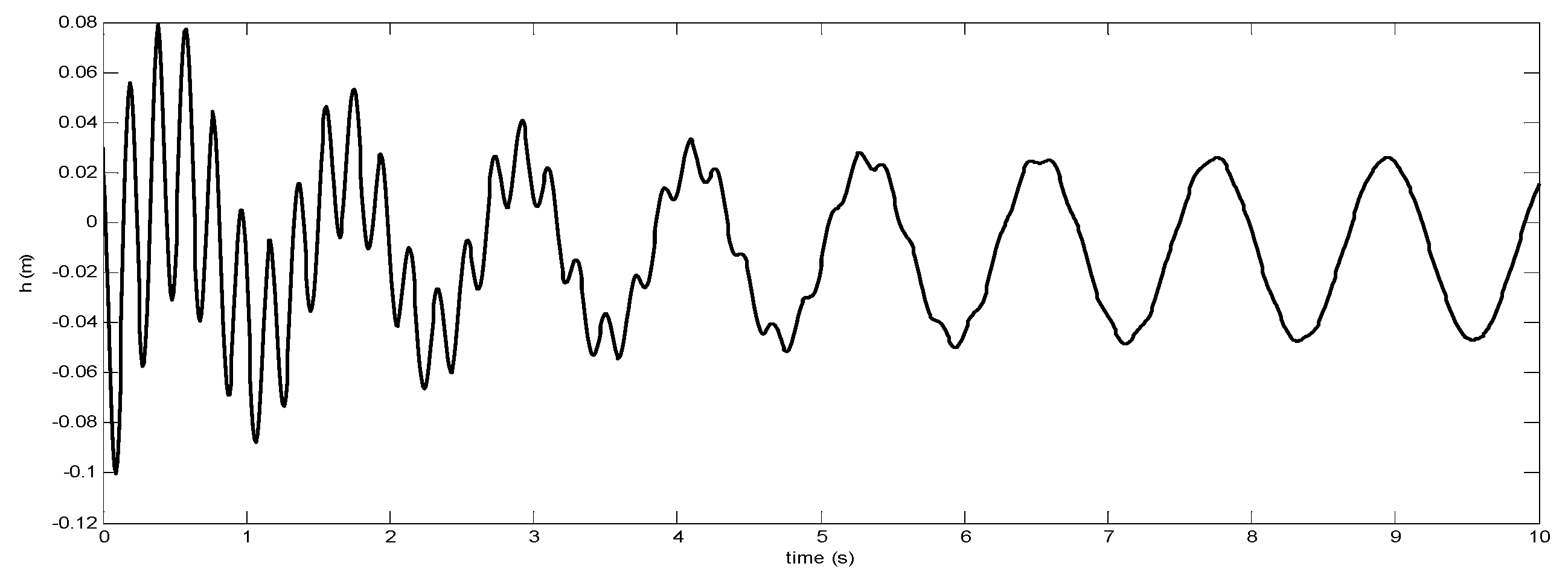
Figure 5,
Figure 6 and
Figure 7 show the results for the speed of 20 m/s, as shown in these figures the results are converging for all three variables.
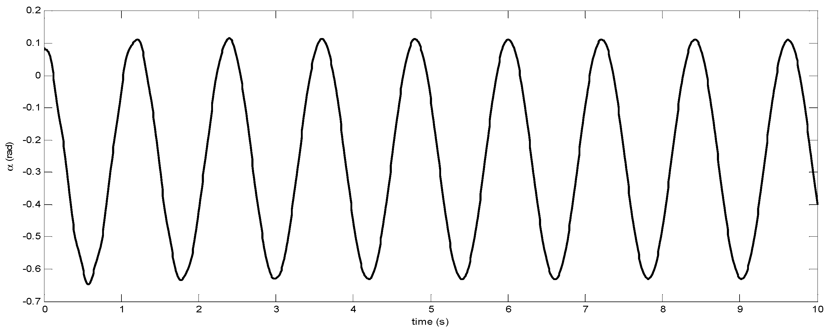
Figure 8,
Figure 9 and
Figure 10 show the oscillatory time responses with constant amplitude (which occurs in the flutter speed) for the speed of 23.9 m/s.
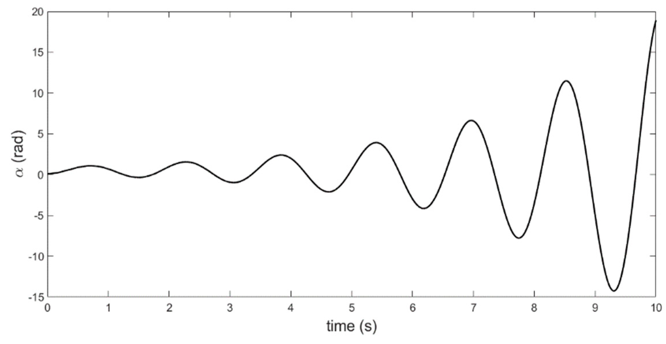
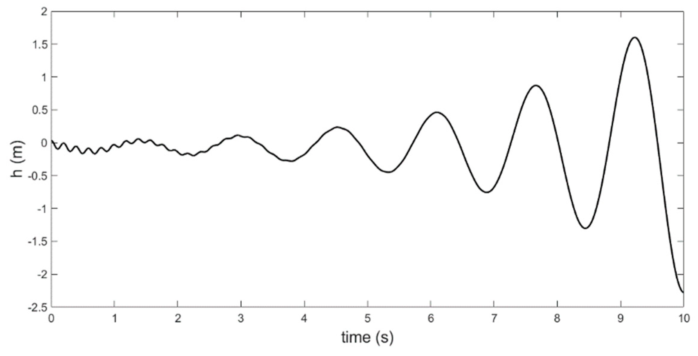
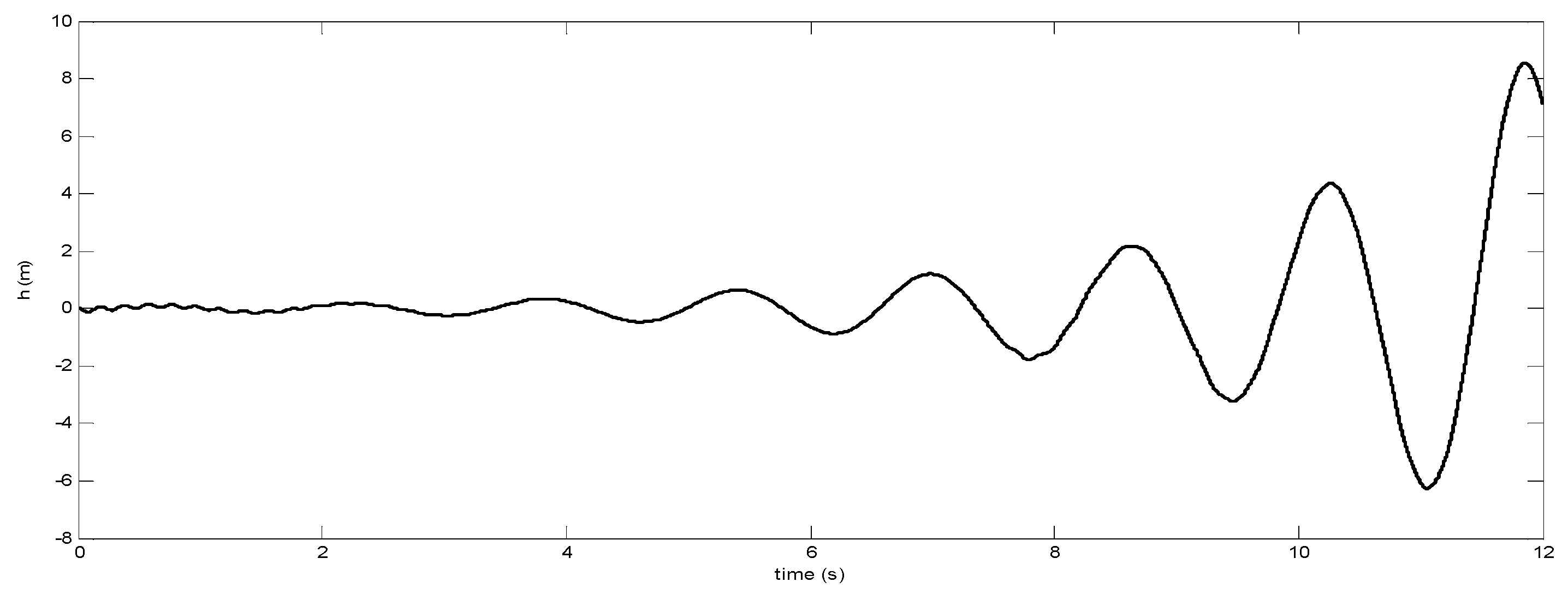
Figure 11,
Figure 12 and
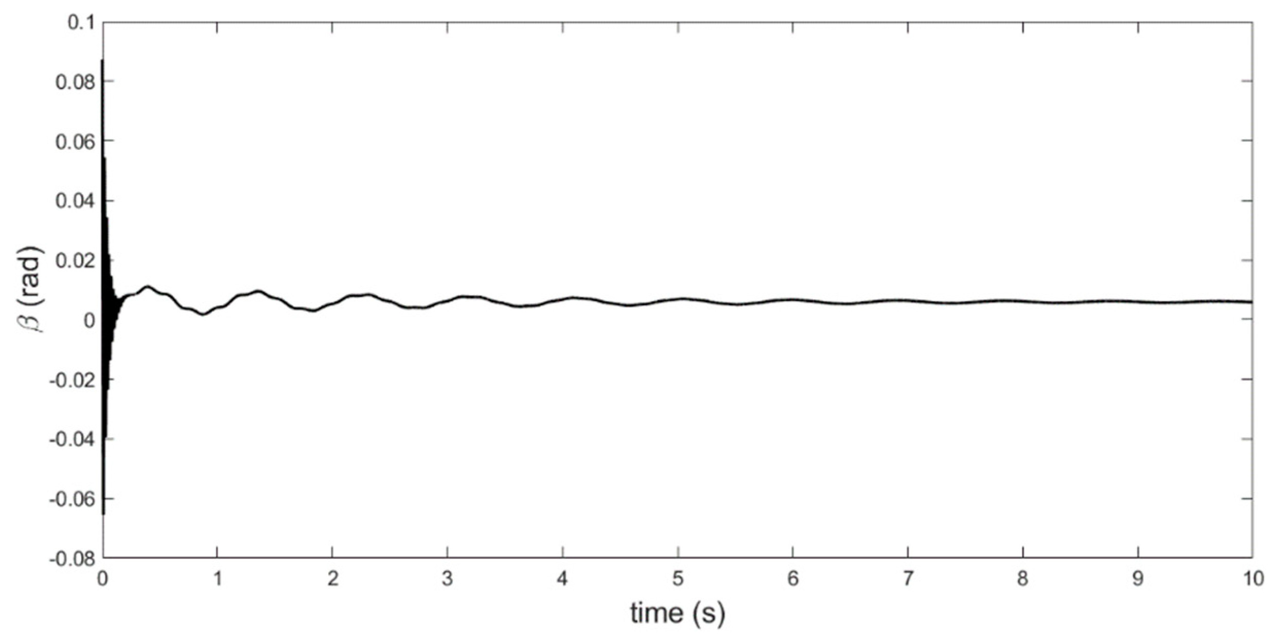
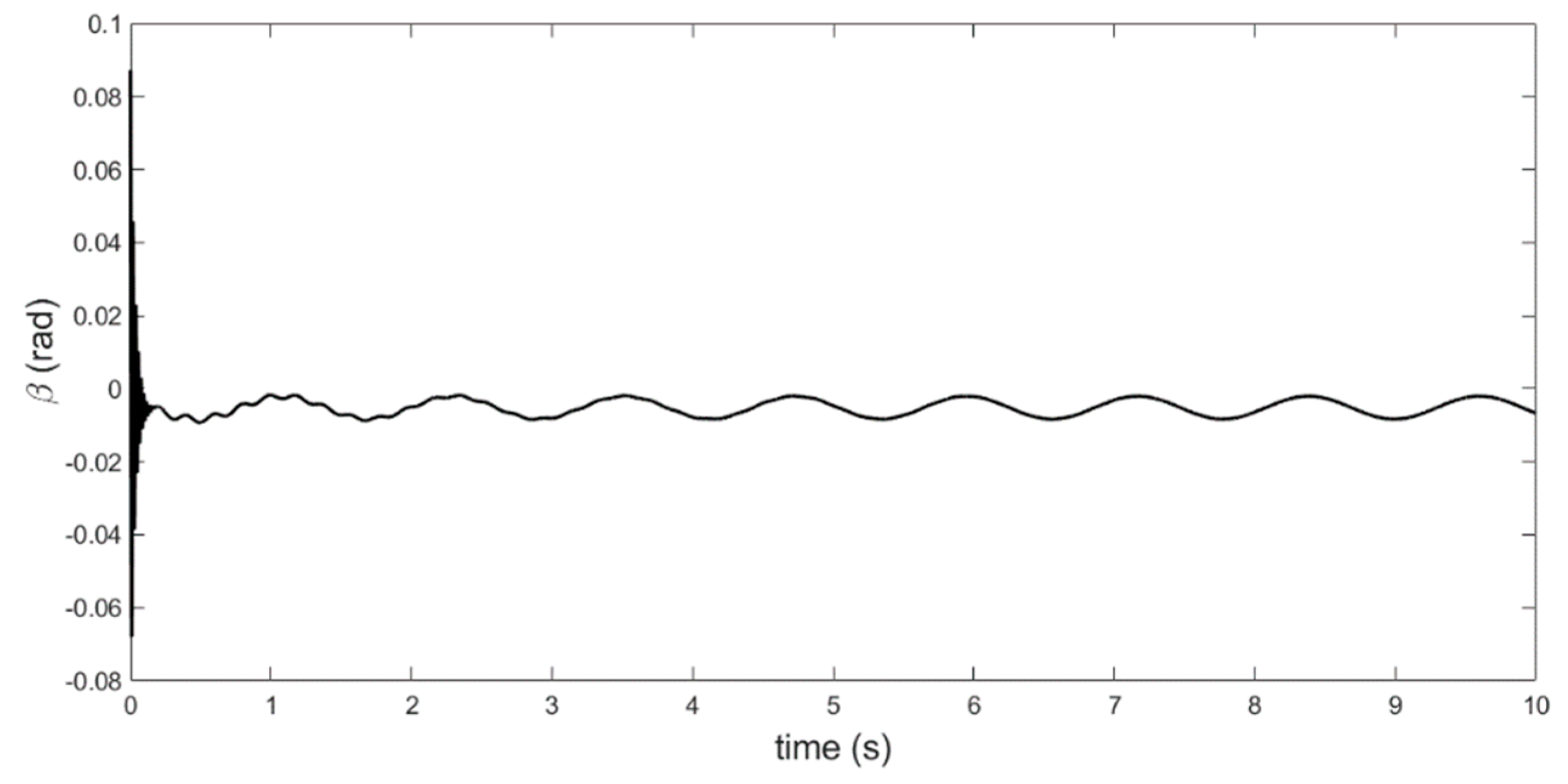
Figure 13 confirm that the time response results of all three variables diverged for the speed of 35 m/s.
It is worthwhile to mention that the amount of amplitude of α or torsional mode of airfoil is predominated toward the bending mode or torsional mode of control surface. The results of this section confirm the validity of the used method in modeling and aero-elastic behavior prediction of the airfoil using the concept of flutter speed. Accordingly, the effects of the control surface freeplay will be discussed in the next section.
5.3. The effect of Control Surface Freeplay
The results of numerical simulation considering the freeplay effects are presented in this section. For the flutter analysis with respect to the freeplay effect, the system response time is plotted. As expected, the surface freeplay decreases the flutter speed due to decreasing the equivalent strength of the flap. The flutter speed for two-dimensional airfoil with the freeplay effect became lower with increased LCO up to 23.9 m/s.
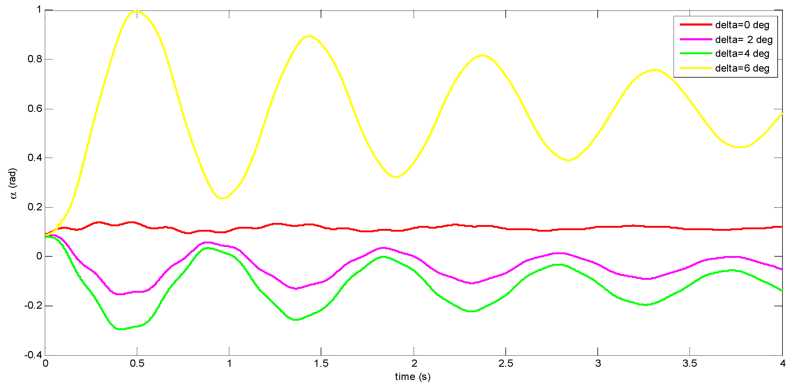
More results are shown in
Figure 23 for different degrees of freeplay to investigate the sensitivity of the results to freeplay degrees. This figure shows that:
the amplitude of oscillation of response in case of freeplay is a bit more than normal;
if the degree of freeplay is more than the response of the primary domain (4 deg for the in hand problem), the time responses change dramatically and create large domain; and,
for freeplay degrees of less than primary domain of response of control surface the time response results are close together, and all of them converged in the lower flutter speed.
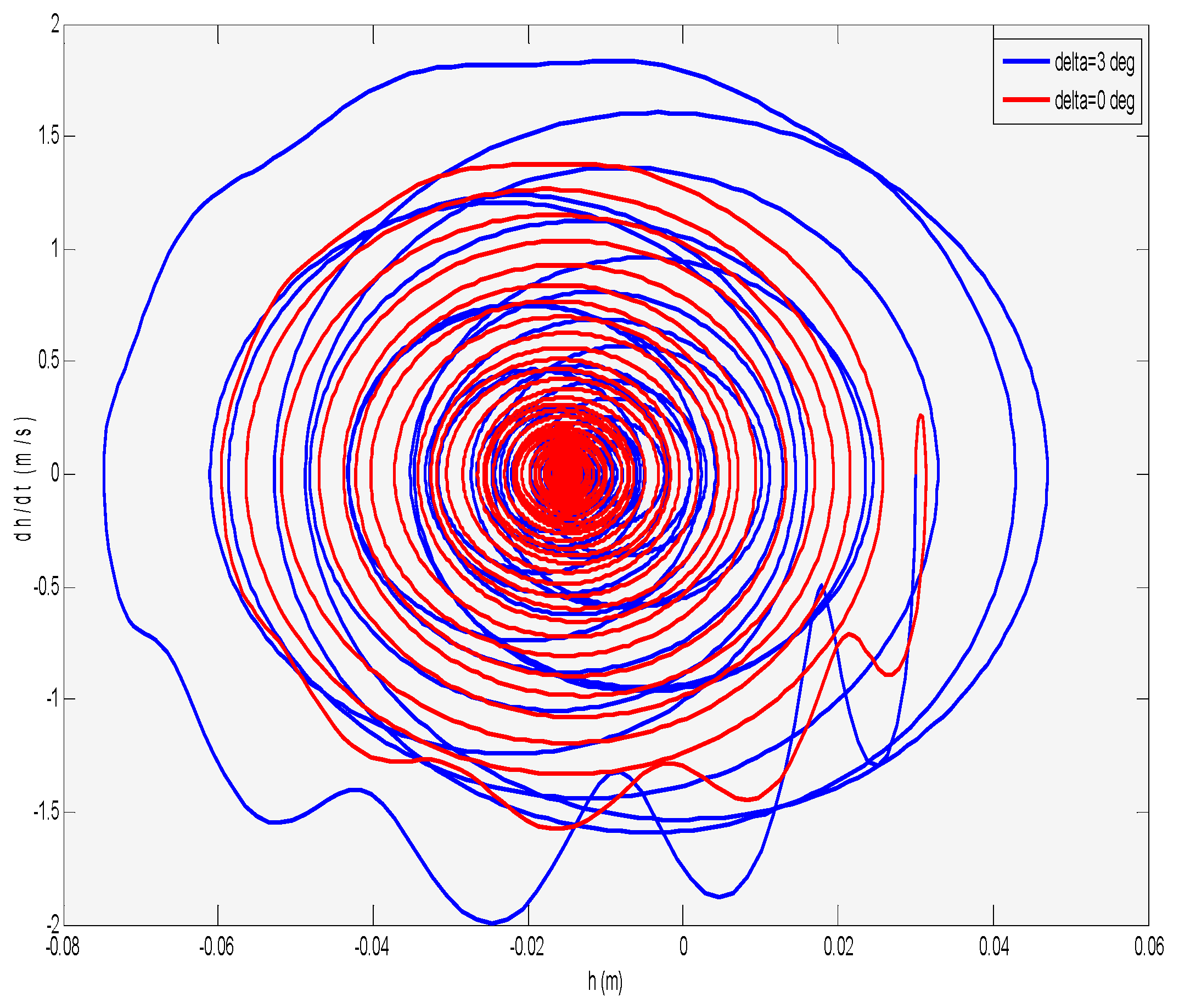
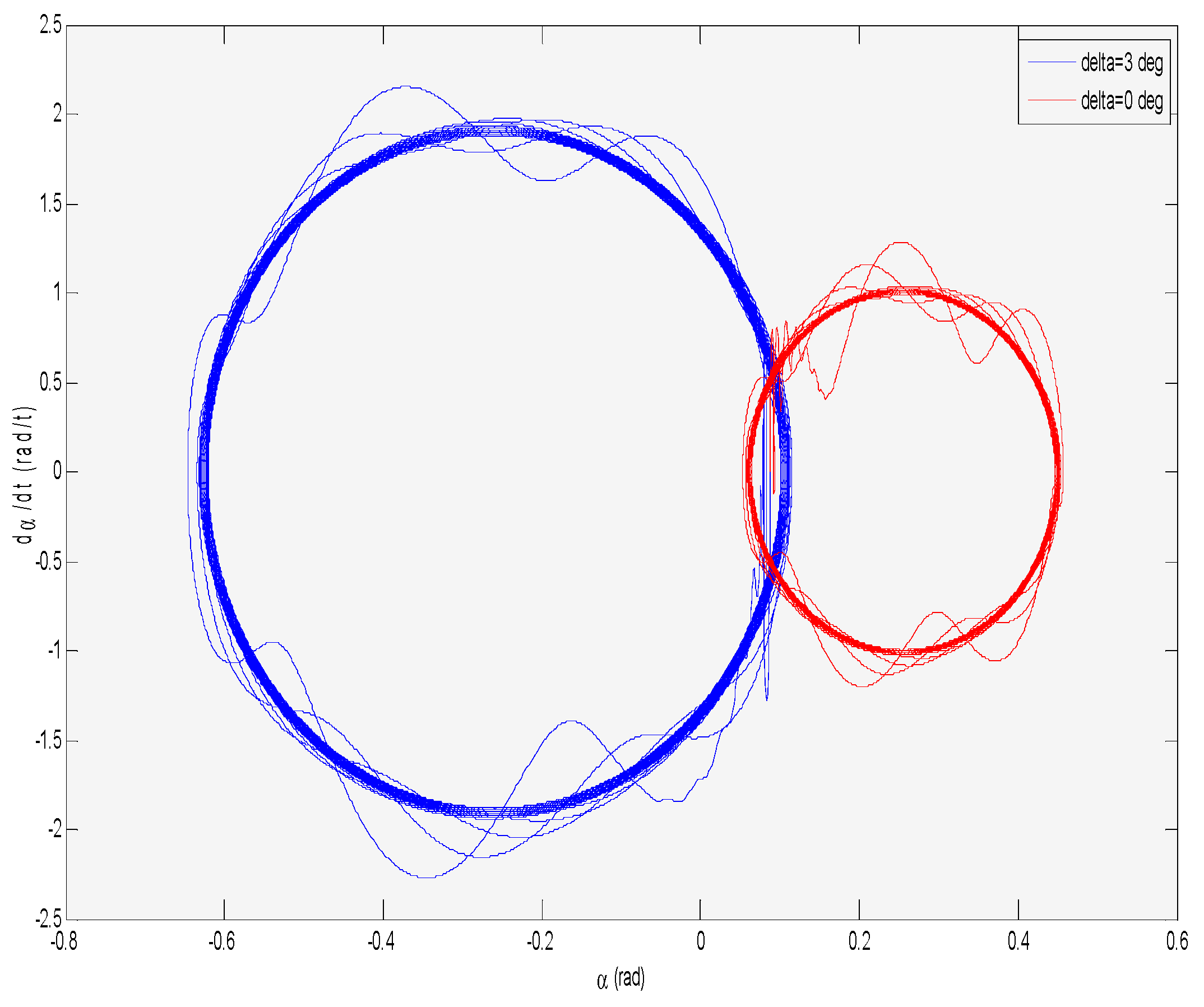
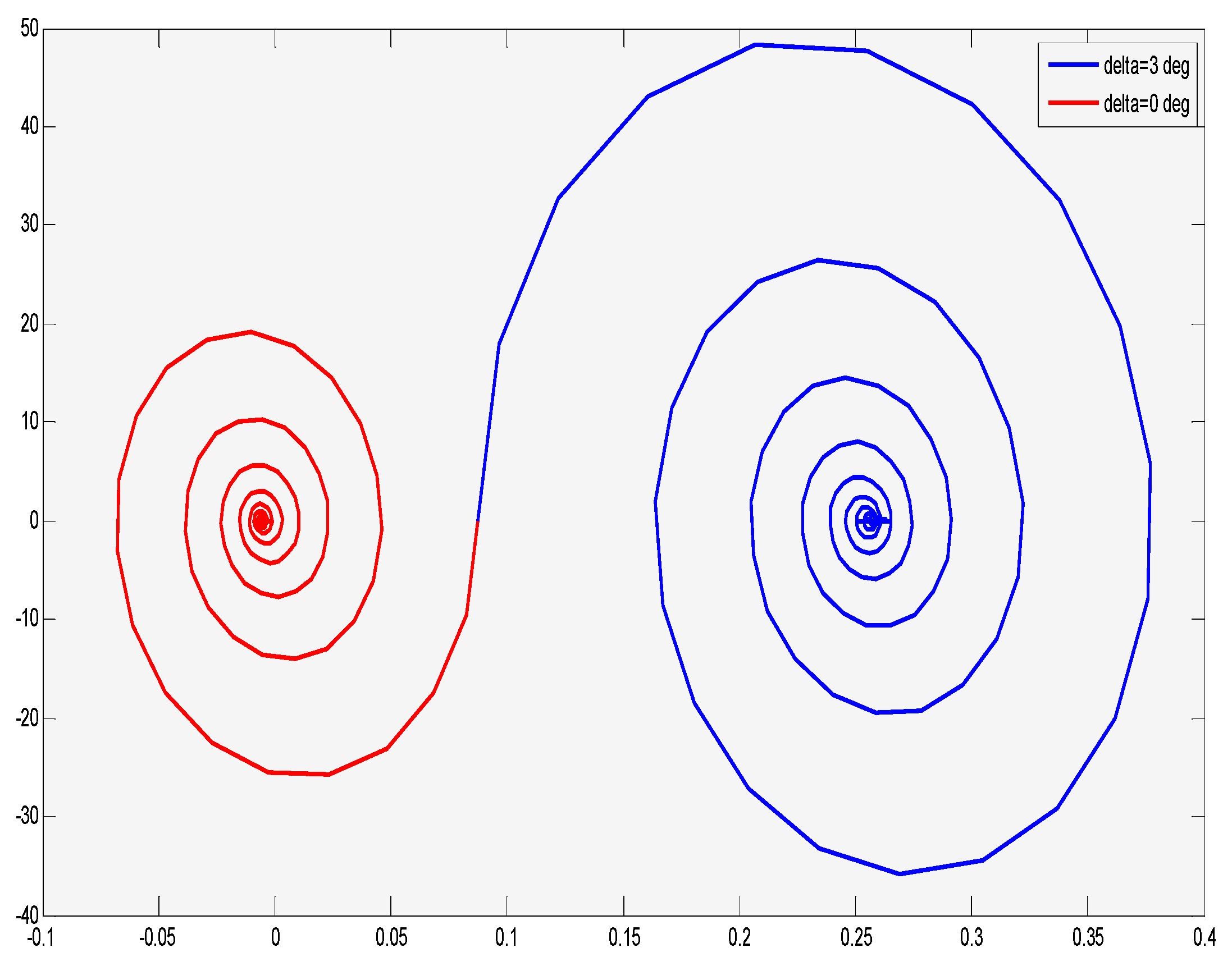
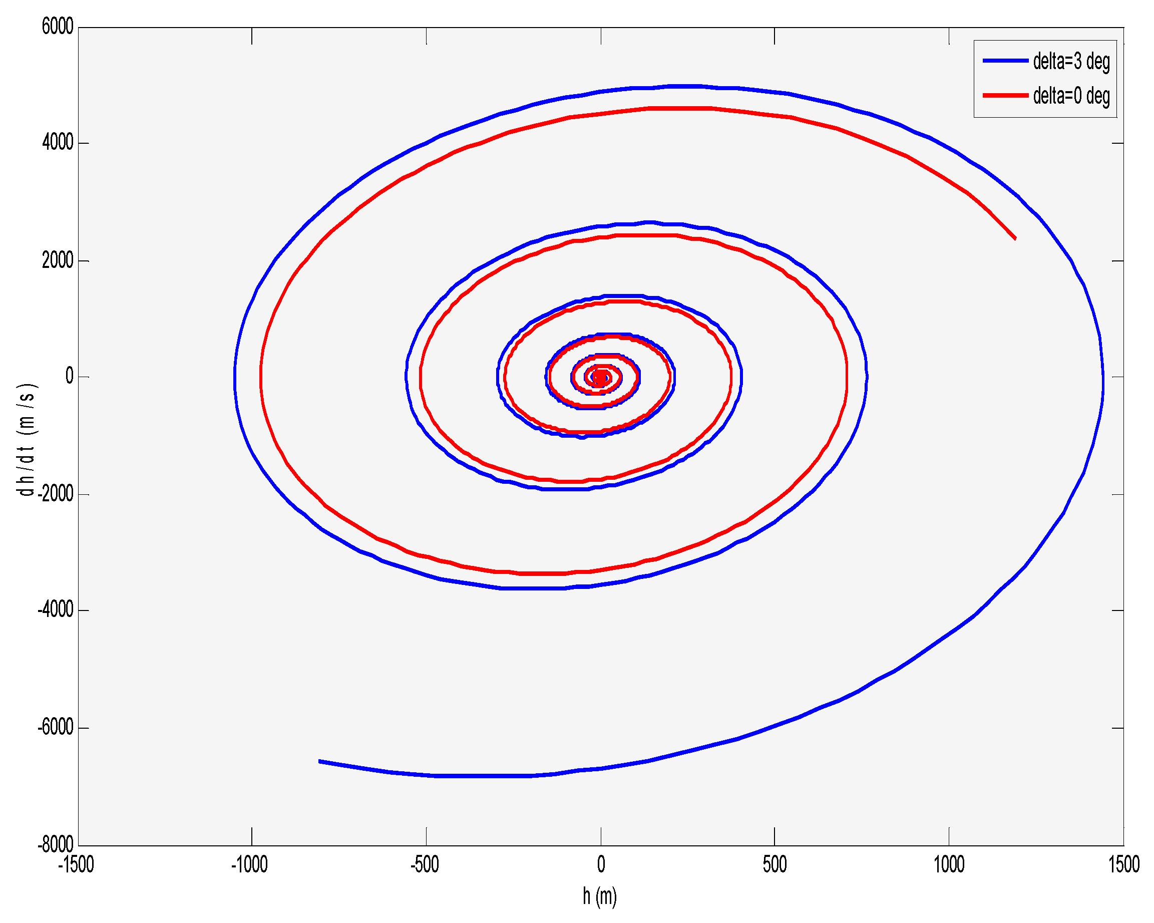
5.4. Stability Analysis
The state space representation is used, as shown in
Figure 24,
Figure 25,
Figure 26,
Figure 27,
Figure 28,
Figure 29,
Figure 30,
Figure 31 and
Figure 32, which presents the responses of α, β, and h for lower, upper, and in the flutter speed in order to study the stability of time responses (without freeplay and with
freeplay). In a lower speed of flutter (
Figure 24,
Figure 25 and
Figure 26), the responses started from the initial value, and converged in the equilibrium point. In the flutter speed (
Figure 27,
Figure 28 and
Figure 29), the response of β has been converged, but the responses of α and h became like rings. This phenomenon occurred, because, in this case, the responses have oscillation, but the domain of oscillations has remained constant. Additionally, in upper speed of flutter (
Figure 30,
Figure 31 and
Figure 32), the responses diverged over time and trend to infinite.
5.5. Validation of the Results
This section compares the results that were obtained from the current work with those of other published studies in order to confirm the validity of the proposed approach.
Table 4 shows the summary of this comparison. This table clearly confirms that the proposed approach can predict the aero-elastic behavior of complex geometry in incompressible flow with reasonable accuracy in comparison with other huge and complex algorithms and experimental methods.
6. Conclusions
This paper focused on a new low-cost method for prediction of aero-elastic behavior of complex geometry in incompressible flow with a reasonable level of accuracy. First, a two-dimensional aero-elastic airfoil model with control surface freeplay (based on Theodorsen method, Lagrange method, and Jones approximation) was developed and the generated equations were solved while using numerical integration. After checking the validity of the generated model (converging behavior in lower flutter speed, oscillatory response with constant amplitude at flutter speed, and diverging at speeds upper than flutter), the freeplay was added to the equations. In the absence of the freeplay, the P-method could be used to find the flutter speed, as the equations are linear. In the case of the freeplay effect, the time response approach is used for flutter analysis. The results showed that the flutter speed for two-dimensional airfoil without freeplay is 23.9 m/s, which is in a very good agreement with publicly available studies. In the presence of freeplay, the oscillations start at a lower speed and the amplitude of the oscillation for a particular initial condition is strongly dependent on the amount of free-play. It is also worthwhile to mention that the system response could be flutter, LCO, or chaotic, depending on the geometrical property, system inertia, and the initial velocity of the system.


