Article

A Generalized State-Space Aeroservoelastic Model Based on Tangential Interpolation

by
David Quero
1,*,
Pierre Vuillemin
2 and
Charles Poussot-Vassal
2
1
Institute of Aeroelasticity, DLR (German Aerospace Center), 37073 Göttingen, Germany
2
DTIS (Information Processing and Systems), ONERA (French Aerospace Lab), Université de Toulouse, 31055 Toulouse, France
*
Author to whom correspondence should be addressed.
Aerospace 2019, 6(1), 9; https://doi.org/10.3390/aerospace6010009
Submission received: 27 November 2018 / Accepted: 11 January 2019 / Published: 15 January 2019
(This article belongs to the Special Issue Aeroelasticity)

Abstract

:
In this work, a new approach for the generation of a generalized state-space aeroservoelastic model based on tangential interpolation is presented. The resulting system of differential algebraic equations (DAE) is reduced to a set of ordinary differential equations (ODE) by residualization of the non-proper part of the transfer function matrix. The generalized state-space is of minimal order and allows for the application of the force summation method (FSM) for the aircraft loads recovery. Compared to the classical rational function approximation (RFA) approach, the presented method provides a minimal order realization with exact interpolation of the unsteady aerodynamic forces in tangential directions, avoiding any selection of poles (lag states). The new approach is applied first for the generation of an aerodynamic model for the bidimensional unsteady incompressible flow in the time domain. Next, an application on the generation of an aeroservoelastic model for loads evaluation of the flutter reduced order assessment (FERMAT) model under atmospheric disturbances is done, showing an excellent agreement with the reference model in the frequency domain. The proposed aeroservoelastic model of minimal order is suited for loads analysis and multivariable control design, and an application to a gust loads alleviation (GLA) strategy is shown.

Graphical Abstract

1. Introduction

One of the major tasks for aircraft certification is the consideration of dynamic load cases, in particular those caused by gust and continuous turbulence encounters. The scenarios to be considered are specified by the regulatory agencies [1,2]. Typically, the sizing of the aircraft components is determined by different loadings corresponding to different excitations and both discrete gust and continuous turbulence are of major importance. In order to reduce the internal loads caused by these atmospheric disturbances without compromising the structural weight, different load alleviation schemes are applied. For modern transport aircraft configurations, an accurate model suited for the design of advance control laws covering the complete flight envelope is of most relevance, as the physical effects governed by the subsonic and transonic flow surrounding the aircraft structure must be precisely described. Thus, the need arises for an accurate but at the same time efficient model description over the complete flight envelope in order to design suitable control laws for an appropriate load reduction when encountering atmospheric disturbances. Moreover, modern transport aircraft are becoming more flexible and, as a result, the low frequency flexible modes tend to interact with the rigid-body behaviour of the structure. Thus, a model description containing the rigid and flexible effects should be taken into account for an effective control design.
Modern approaches of control theory require a description of the model in the time domain. However, the aerodynamic models describing the flow over the aircraft are provided within the frequency domain in tabular form as they cannot usually be obtained in an explicit form and, if they are, they contain transcendental functions which cannot be transformed in the time domain by a direct application of an inverse Laplace transform. Thus, there is a need for converting the frequency-domain description into time-domain models. For the application of the control theory techniques, it is moreover desirable that the size of the time-domain description is kept minimal.
Historically, the unsteady subsonic air forces for three-dimensional configurations have been determined for pure harmonic motion. For analytic functions in the frequency domain, the function in the whole complex plane defined by the Laplace variable s can be then deduced from the values over the imaginary axis i ω for pure harmonic motion [3]. The method of Roger [4] and Abel [5], based on a rational function approximation (RFA), represents the three-dimensional subsonic aerodynamic by means of a least-squares technique with a series of poles which represent the aerodynamic lags due to the presence of the wake. All elements of the transfer function matrix share the same poles, which in turn have to be chosen in advance. Note that the least-squares fit is ill-conditioned when increasing the number of real poles and is prone to numerical instabilities [6,7]. When applied at a half-generalized level in an effort not to increase the size of the state-space model, the least-squares fit for the gust excitation shows additional issues related to the time delay behaviour of the input. To overcome this problem, some authors divide the gust input in different zones along the flight direction and thereby increase the number of effective inputs [8,9]. Other authors apply an interpolation for the distributed aerodynamic loads, avoiding the delay term to be included in the frequency-domain description at the cost of drastically increasing the number of states [10,11]. In order to take into account the poles as free parameters to the least-squares fit, they can be further considered in an optimization problem [12,13], ensuring a minimum error of the least-squares for a fixed number of poles. Karpel presented the minimum-state method [14], where an iterative least-squares process is applied to the aeroelastic system, reducing the total number of augmented states. This iterative process leads to a significant increase of the computational effort which may be of up to three orders of magnitude [3].
Regarding the load alleviation strategies, the objective function to be minimized for a controller synthesis is a set of cut loads acting at specific aircraft locations. There are two common ways to compute the nodal loads acting over the airframe, namely the mode displacement method (MDM) and the force summation method (FSM) [15]. Several authors [15,16] showed that the FSM method has a superior convergence with respect to the number of structural modes retained for the projection of the aeroelastic equation. As discussed by Castrichini et al. [11], the MDM is not appropriate for cases where the loads are not smoothly distributed over the aircraft structural model, as the load distribution is not close to orthogonal for high frequency structural modes in that case, as they are characterized by significant spatial waviness. The structural modes selected for the projection of the aeroelastic equation correspond to the unloaded structure and therefore they are not influenced by the applied loads, leading to the selected modal basis to be not suitable to represent generic load distributions. It is common practice to consider the generalized and not the distributed aerodynamic forces for the aeroservoelastic system in the time domain in order to improve the least-squares solution by a reduced number of quantities to be fitted [8], leading to the application of the MDM for the cut loads recovery as a unique option, requiring the FSM method the knowledge of the aerodynamic loads distribution. As a consequence, modern techniques of the control theory are applied to aeroelastic systems where the loads recovery is done by means of the MDM [17], even though the FSM method has a superior convergence of the cut loads’ values with respect to the number of structural modes considered. For the FSM method, the challenge consists of properly modeling the unsteady distributed aerodynamic loads and this is achieved by the present method.
In general, all the RFA methods introduce an error in the description of the aerodynamic loads due to the least-squares fit. In order to avoid this error, different techniques based on rational interpolation may be used. More recently, the Eigensystem Realization Algorithm (ERA) algorithm [18] has been widely used for system identification and model reduction [19,20] in the time domain. As stated by Ma et al. [21], the ERA algorithm produces theoretically the same reduced-order models as balanced proper orthogonal decomposition (POD) [22] with no need of an adjoint system. It can also be regarded as the data-driven approximation to balanced truncation [23]. As a rational interpolation technique, it can be considered as a rational interpolant at infinite frequency [24]. There are two main difficulties associated with the ERA application. Firstly, its application is limited to proper systems and thus only the MDM method can be considered for the loads recovery. Secondly, if the system under consideration has a large number of inputs and outputs, then a big computational effort is required to compute the singular value decomposition (SVD) of the dense and large-size Hankel matrix [23].
For the consideration of linear time-invariant (LTI) multi-input multi-output (MIMO) systems with a non-proper transfer function matrix, a more general setting, namely that of the linear descriptor systems, is needed [25]. Additionally, the approach presented in this work is based on the Loewner framework, which is an extension of the rational interpolation at infinite frequency to a set of frequencies available at particular values [24].
In this work, a novel approach to generate an aeroservoelastic state-space model suited for loads computation and control design which overcomes the above limitations is presented. The proposed approach shall fulfill the following properties:
  • There is no need for poles selection (lag states). On the one hand, the classical selection of real poles for the RFA techniques does not allow for describing phenomena which present resonance behaviour or peaks in the frequency-domain description at frequencies higher than zero. On the other hand, the set of real poles causes the RFA least-squares fit to be ill-conditioned, and care must be taken when increasing the number of poles. To overcome these limitations, within the present approach, neither a pole selection is required nor the transfer function is limited to a set of rational functions with real poles (see Section 3.1).
  • It provides a small-size generalized state-space representation. The term generalized refers here to the fact that the theory of linear descriptor systems is needed for the present approach (see Section 2.1). This term should not be confused with the term generalized of the aeroelastic equation, where the physical equation is projected onto the set of generalized coordinates corresponding to the modes of the structure in vacuum. The proposed approach can be a regarded as providing a reduced order model (ROM) in the time domain, as it enables solving the aeroservoelastic system in a very efficient way. This is achieved by the condition of minimality of the rational interpolant within the Loewner framework theory [25].
  • It is applicable to (input) delay systems, in particular when the excitation is due to gust disturbances. As described above, RFA techniques based on a least-squares fit of the frequency-domain data are not suited for a gust disturbance input. Two practical solutions in order to avoid this limitation of the RFA techniques, namely dividing the gust excitation in zones or applying a least-squares fit to the distributed aerodynamic nodal loads, may dramatically increase the size of the aeroelastic model in the time domain.
  • It includes rigid-body modes, explicitly dealing with the singularity caused by the translational aircraft motion at zero frequency. This problem has been considered by Karpel et al. [26] in the frequency domain. In this work, the aerodynamic transfer function matrix is modified to include the derivatives of the translational motion previous to the time-domain realization.
  • It is computationally efficient when generating the state-space. Unlike classical approaches where the precision is increased at the cost of an iterative approach [14], the current approach does not require any iterative process. In addition, the computational effort is drastically reduced compared to the ERA method by the consideration of tangential interpolation data within the Loewner pencil [25], avoiding the use of the dense and large-size Hankel matrix.
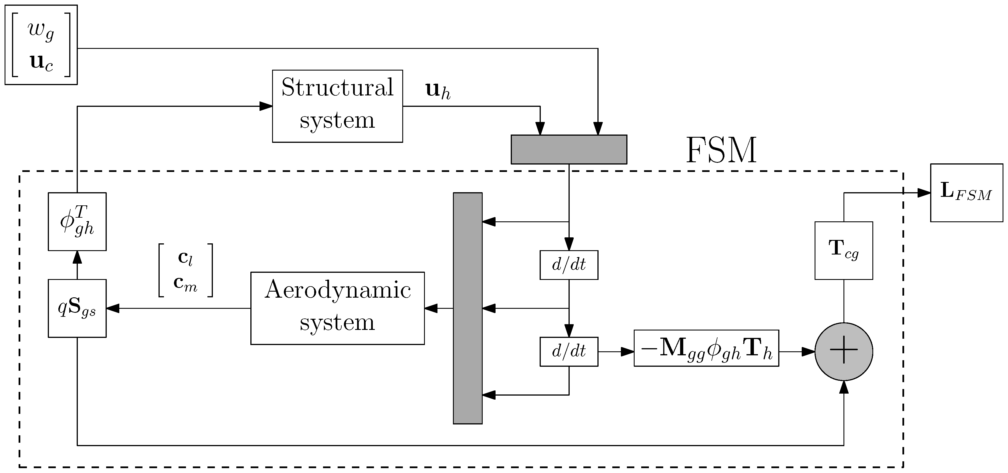
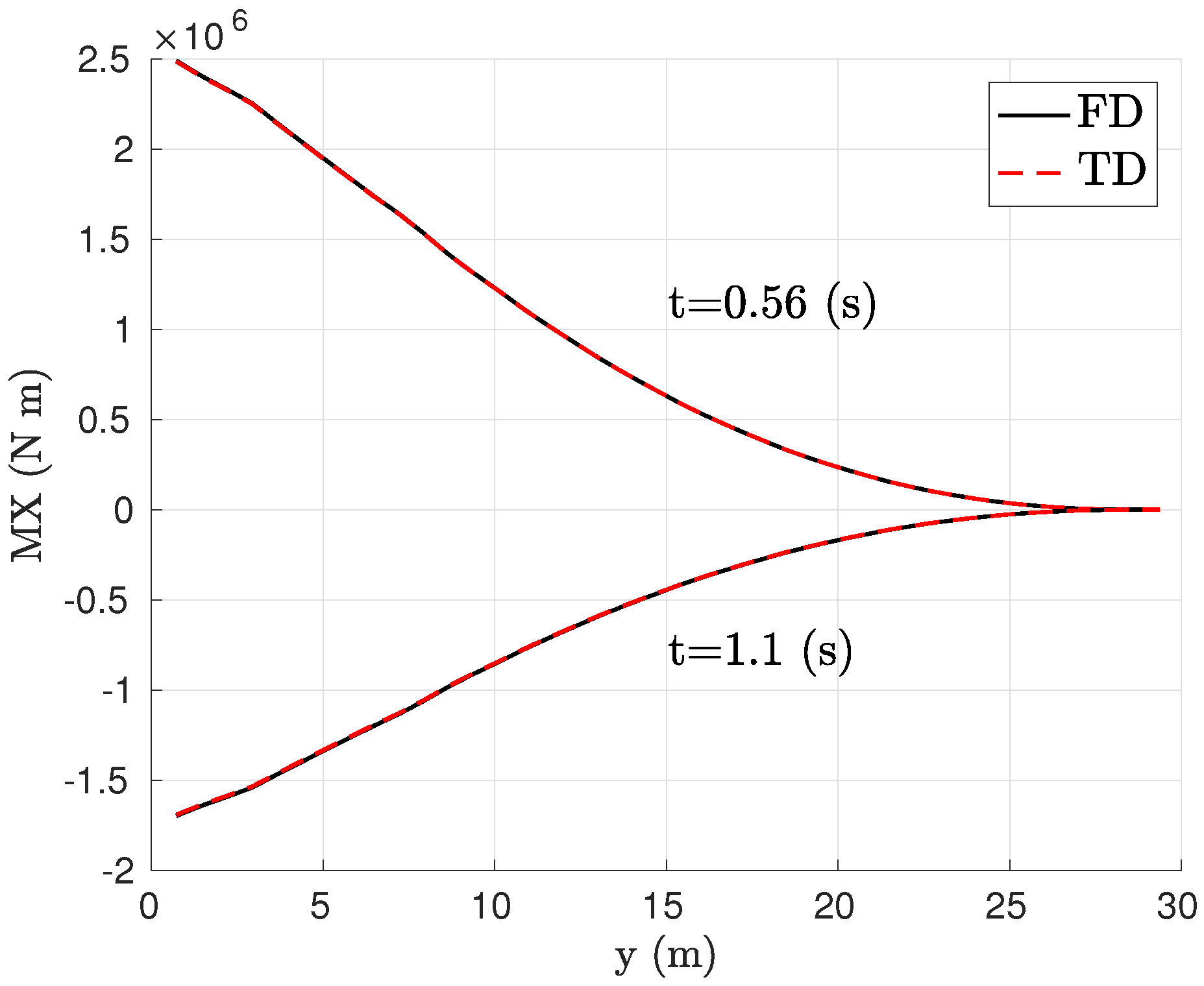
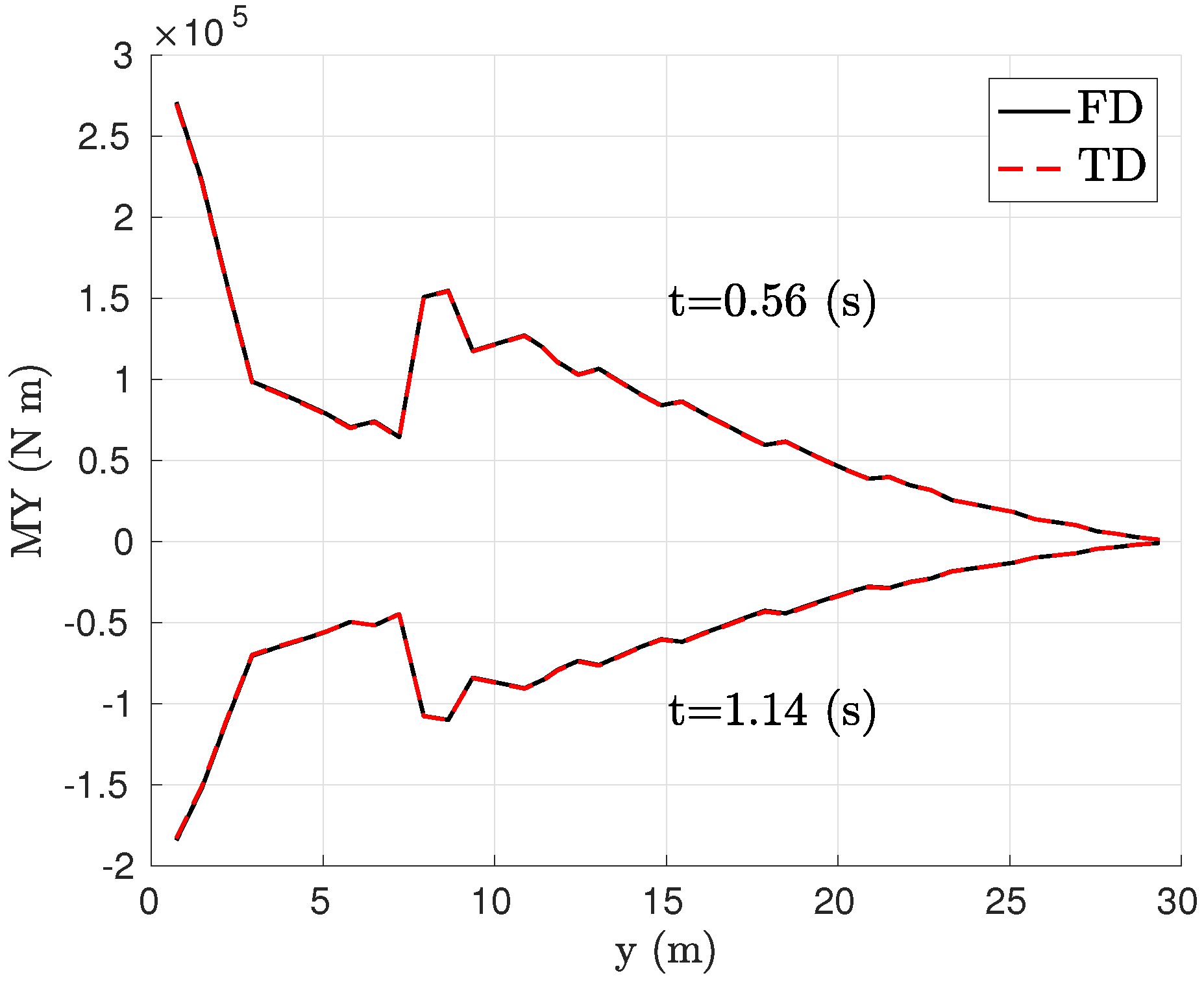
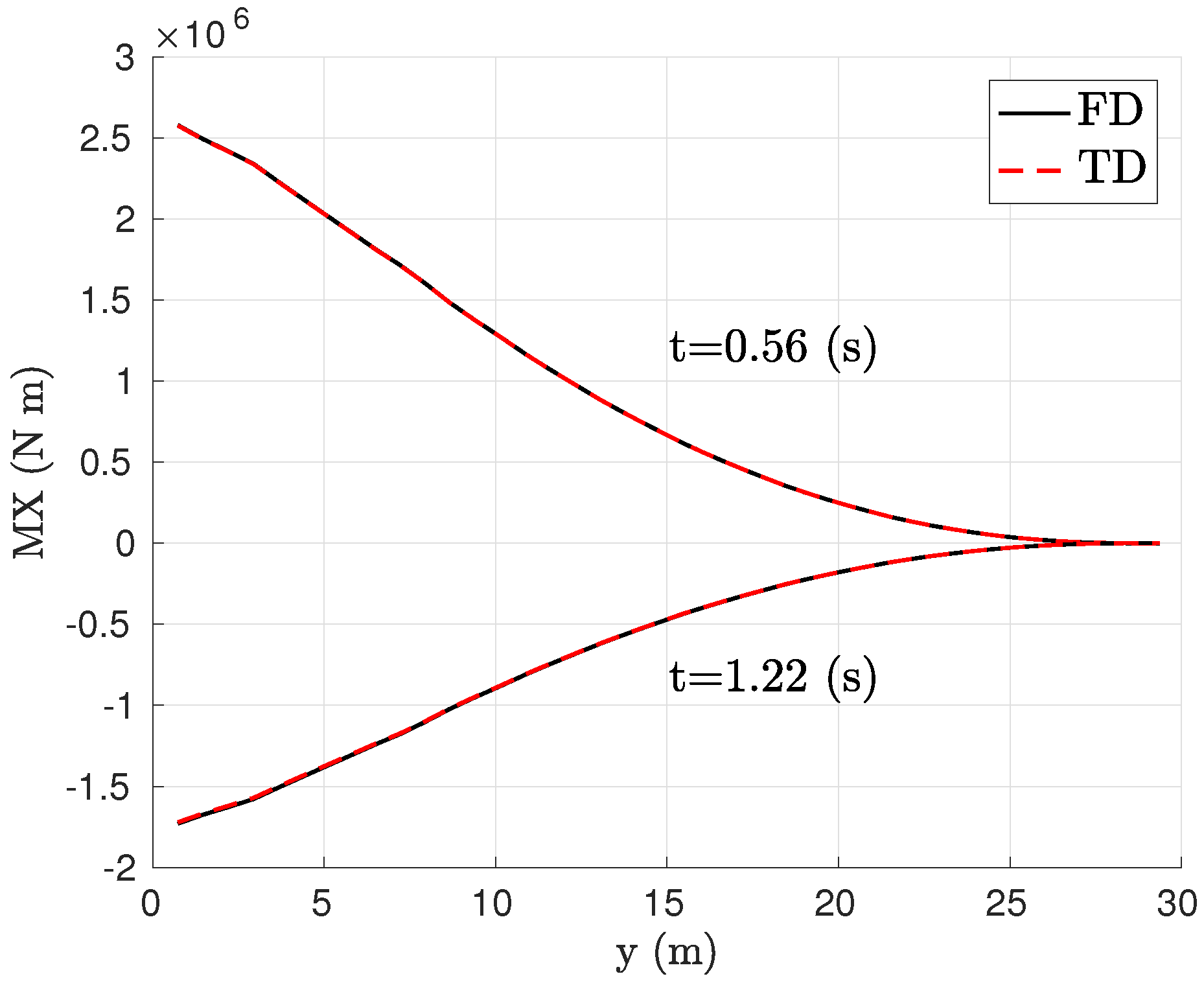
  • It recovers the cut loads by means of the FSM. In order to achieve this, the unsteady aerodynamic loads distribution over the aircraft must be represented in the time domain. As described above, the FSM method is known to have a superior convergence for the cut loads prediction compared to the MDM method commonly used in applications for gust load alleviation (GLA) design [27].
In Section 2, the Loewner realization in connection with the theory of descriptor linear systems is presented and an application to the bidimensional unsteady incompressible flow over an airfoil is shown. A generalization to general three-dimensional aeroservoelastic systems is then presented in Section 3 with special focus on the representation of the distributed unsteady aerodynamic forces in the time domain. In Section 4, applications to the flutter reduced order assessment (FERMAT) model are shown and finally conclusions and future work are pointed out in Section 5.

2. Generalized Realization Problem

2.1. Tangential Interpolation

A linear time-invariant descriptor system S n = E , A , B , C , D is described in the time domain by a set of differential and algebraic equations (DAE), also denoted as a generalized state-space system:
S n : E x ˙ t = A x t + B u t , y t = C x t + D u t ,
where x t R n is the state vector, u t R n u the input vector, E , A R n × n , B R n × n u , C R n y × n and D R n y × n u are constant matrices with E possibly singular. In this work, regular systems are considered, that is, det s E A 0 , except for a finite number of eigenvalues (which may have an infinite value), denoted by the set σ E , A . The resolvent set ρ E , A is given by ρ E , A = C \ σ E , A .
The transfer function matrix H S n s of the system S n is:
H S n s = C s E A 1 B + D .
For the sake of clarity, the transfer function H S n s for the system S n is also denoted as H s . The transfer function is said to be proper if lim s H s is bounded (< for each of its components) and strictly proper if lim s H s = 0 . If the DAE system is split into the fast H s (including only the poles with infinite value) and slow subsystems H p s (including only the poles with finite value) and restricted system equivalence relations are applied so that H s = H p s + H s , the non-proper part of the transfer function matrix H s can be written as a Neumann series expansion [28]:
H s = C s N I 1 B + D = D C B j = 1 υ 1 s j C N j B ,
where N is a nilpotent matrix with nilpotence index υ . This provides a direct relation between the also called DAE index υ and the non-proper part of the transfer function matrix H s , with ν one order less than that of the highest polynomial term.
The set of all possible minimal realizations of H S n of size n is denoted by S n such that S n = E , A , B , C , D S n . The minimal realization of size n used here is based on the rational interpolation for tangential data [25] and the description of the tangential interpolation problem is based on that provided by Lefteriu et al. [29]. Tangential interpolation is a form of rational interpolation where the data is interpolated along particular directions. In particular, the data consist of the right interpolation data:
λ i , r i , w i λ i C , r i C n y × 1 , w i C n u × 1 ,
for i = 1 , , n r :
Λ = diag λ 1 , , λ n r C n r × n r , R = r 1 , , r n r C n u × n r , W = w 1 , , w n r C n y × n r ,
and the left interpolation data:
μ j , l j , v j μ j C , l j C 1 × n u , v j C 1 × n y ,
for j = 1 , , n l :
M = diag μ 1 , , μ n l C n l × n l , L = l 1 T , , l n l T T C n l × n y , V = v 1 T , , v n l T T C n l × n u .
The transfer function matrix is evaluated at the values λ i , μ j and the vectors r i , l j are referred to as right and left tangential directions, while w i , v j are the right and left tangential data. The rational interpolation problem for tangential data aims at finding a realization S n = E , A , B , C , D S n such that the associated transfer function H satisfies the right and left constraints,
H λ i r i = w i , i = 1 , , n r , l j H μ j = v j , j = 1 , , n l ,
which is achieved by means of the Loewner and shifted Loewner matrices. Next, the structure of these two matrices is described.
A set Z of points in the complex plane Z = z 1 , z n r + n l and the corresponding values of the transfer function matrix is partitioned into the left and right data:
Z = λ 1 , , λ n r μ 1 , , μ n l ,
where the total number of sample points is n r + n l . The Loewner matrix is built as:
L = v 1 r 1 l 1 w 1 μ 1 λ 1 v 1 r n r l 1 w n r μ 1 λ n r v n l r 1 l n l w 1 μ n l λ 1 v n l r n r l p w n r μ n l λ n r ,
and satisfies the Sylvester equation:
L Λ M L = L W V R .
The Loewner matrix can be also expressed in terms of the tangential controllability and observability matrices [29]. If the directions r i , l j are selected generically (random in practice), the rank of the Loewner matrix L is equal to the rank of the underlying matrix E . The shifted Loewner matrix is the Loewner matrix corresponding to s H s and is built as:
L σ = μ 1 v 1 r 1 λ 1 l 1 w 1 μ 1 λ 1 μ 1 v 1 r n r λ n r l 1 w n r μ 1 λ n r μ n l v n l r 1 λ 1 l n l w 1 μ n l λ 1 μ n l v n l r n r λ n r l n l w n r μ n l λ n r ,
and satisfies the Sylvester equation:
L σ Λ M L σ = L W Λ M V R .
Assuming that n r = n l and that det L σ s L 0 a minimal realization S n = E , A , B , C , D S n for the linear descriptor system is given by [25]:
E = L , A = L σ , B = V , C = W , D = 0 ,
and the associated transfer function H s = W L σ s L 1 V satisfies the right and left interpolation conditions of Equation (3). An additional SVD factorization of the Loewner matrix L allows for the further size reduction of the system, generating a reduced order model (ROM) of the descriptor system:
L = Y 1 Y 2 Σ 1 0 0 Σ 2 X 1 * X 2 * ,
where * denotes the conjugate transpose, Σ 1 R r × r , Σ 2 R n r × n r and X 1 , X 2 , Y 1 , Y 2 are of appropriate dimensions. The reduced system of size r defined by S r = E r , A r , B r , C r , D r S r is obtained by a Petrov–Galerkin projection and represents the best approximation to the full Loewner matrix in the Frobenius or 2-norm:
E r = Y 1 * L X 1 , A r = X 1 * L σ X 1 , B r = Y 1 * V , C r = W X 1 , D r = 0 .
As a remark, note that the rational interpolation problem is different from the classical one of rational approximation. In the framework of rational interpolation presented here, the generalized system obtained by the Loewner realization exactly interpolates the transfer function matrix H given at the sample points in tangential directions, satisfying the conditions given in Equation (3). The rational approximation instead provides a least-squares fit to the data and thus a systematic error is introduced. As a result, some authors impose additional constraints (usually at zero or flutter frequencies) to improve the fit [13]. In order not to deteriorate the fit at other frequencies, the number of terms for the least-squares fit must then be increased.
Once the system S r = E r , A r , B r , C r , D r S r has been determined, it may contain unstable poles. Assuming that the aeroservoelastic system under consideration is stable, the system is then approximated by a stable one. This is done by means of an approximation in the space of rational functions contained in the Hardy space H as described in Section 2.2.

2.2. Optimal R H Approximation

The following classes of descriptor systems are defined:
S 0 = E r , A r , B r , C r , D r S r ρ E r , A r i R = ϕ , S + = E + , A + , B + , C + , D + S r ρ E + , A + C + , S = E , A , B , C , D S r ρ E , A C ,
where ϕ is the empty set, ρ E , A the resolvent set as described in Section 2.1, S r represents all realizations of size r as in Equation (7), S + represents the class of stable descriptor systems and S represents the class of unstable descriptor systems, both of size r. The system obtained from tangential interpolation as specified in Equation (7) may contain artificial unstable poles, in the sense that the original system is stable, as the method described in Section 2.1 does not preserve stability. Assuming that the reduced system S r obtained by Equation (7) does not contain any poles in the imaginary axis ( S r S 0 ), the problem of finding the best approximation of the system S r by a stable system S ^ r + S + minimizes the distance between the transfer function matrices H :
S ^ r + = arg min S S + H S r H S p .
This continuous-time problem has been explicitly solved by Köhler [30], requiring additionally that the matrix E + for the class of stable descriptor systems S S + be invertible, that is, with a proper transfer function matrix such that lim s H S s is bounded (< for each of its components). The subindex p 2 , represents the norm to be minimized in the corresponding Hardy space H p . The space R H includes all stable bounded rational transfer function matrices H in the Hardy space H ( p = ) of analytic functions in the (open) right half of the complex plane C + :
H = H : C C n y × n u H < , H = sup s C + H s = sup ω R σ m a x H i ω ,
with σ m a x the maximum singular value of the transfer function matrix H i ω .
The optimal solution in the R H space is given by Köhler [30]:
S ^ r + = S r + P S r , σ 1 Q ,
where the system S r + corresponds to the original system S r but keeping solely the stable poles (with negative real part). The system S r , σ 1 S is S r , σ 1 = E r T R 1 , A r T R 1 C r T C 1 , E r T Q B r , C r P E r T , D r with:
C 1 = C r P E r T , R 1 = Q E r P E r T σ 1 2 I ,
and P and Q are the unique infinite gramians that satisfy the following generalized Lyapunov equations:
A r P E r T + E r T P A r T + B r B r T = 0 , A r Q E r + E r T Q A r T + C r T C r T = 0 .
The optimal solution S ^ r + in the R H space verifies that H S r H ( S ^ r + ) = σ 1 , where σ 1 = S r = max P Q is the greatest Hankel singular value of the system S r S which results from the original system S r but keeping solely the unstable poles (with positive real part).

2.3. Application to Unsteady Incompressible Flow

As it is clear from Section 1, the main task for the application of the FSM method for the cut loads recovery in an aeroservoelastic framework remains to properly describe the distributed unsteady aerodynamic forces in the time domain. In order to show the convenience of the tangential interpolation method described in Section 2.1, an application for the incompressible unsteady flow over a bidimensional airfoil with heave and pitch degrees of freedom is presented, showing the connection between the DAE theory or descriptor systems and the unsteady aerodynamic model.
The classical unsteady model of Theodorsen [31] provides the lift and pitch moment coefficient (excluding the added-mass terms) to arbitrary input motions of the airfoil. The Wagner model in the time domain is equivalent to that of Theodorsen in the frequency domain, which uses the physical assumptions of inviscid flow, incompressibility and planar wake. As described by Brunton [32], several authors have constructed state-space models corresponding to the Theodorsen formulation. Note that excluding the models obtained by Peters [33], which requires eight states for an appropriate system representation, these state-space formulations do not include the added-mass terms. In this section, a time-domain model including also the added-mass terms is obtained.
The local lift c l (positive upwards) and local pitch moment at the quarter chord c m (positive nose up) can be described as a function of the heave u z (positive down) and pitch u θ (positive nose up) motion in the frequency domain by means of an aerodynamic transfer function matrix:
c l ω c m ω = H ω u z ω u θ ω ,
where the system output is y = [ c l c m ] T , the system input is u = [ u z u θ ] T and the transfer function matrix is [34]:
H ω = ω 2 π L r e f U 2 + i ω 2 π U C k ω 2 π a L r e f 2 U 2 + i ω π L r e f U 1 + 1 2 a C k + 2 π C k ω 2 π L r e f 4 U 2 ω 2 1 8 a 2 π L r e f 2 2 U 2 i ω π L r e f 2 U ,
where k is the reduced frequency k = ω L r e f / U with L r e f a reference length (the half-chord) and U the true airspeed. The parameter a represents the pitch axis location with respect to the half-chord and ranges between 1 for the leading edge and 1 for the trailing edge. The Theodorsen function C k is given by:
C k = H 1 2 k H 1 2 k + i H 0 2 k ,
with H 0 and H 1 the Hankel functions of first and second kind [31]. Interestingly, the pitch moment at the quarter chord position is independent of the Theodorsen function. Note that, in this work, all time-dependent dynamic variables such as c l , c m , u z and u θ are incremental variables in the sense that they refer to deviations with respect to a steady-state reference.
It is clear from Equation (9) that the aerodynamic system is not proper, as the values lim s H s are not bounded. According to Equation (2), the corresponding time-domain description must be in the form of a descriptor system of index ν 1 = 2 , that is, of index υ = 3 . The generalized realization based on tangential interpolation of Section 2.1 can then be applied. However, it is well known that the numerical time-domain solution of DAE systems becomes very difficult for index values higher than 2 [35] and thus a procedure to reduce the DAE index for this particular aerodynamic system is proposed. With the transfer function matrix given by Equation (9), the DAE index can be reduced by simply reducing the polynomial order at s . Even though the coefficients corresponding to the non-proper polynomial terms in Equation (9) are explicitly known, a general method based on the evaluation of the polynomial coefficients by means of the derivatives of the transfer function matrix H ω with respect to the circular frequency ω is given. This results in a more general setting, as typically the aerodynamic system description is provided at a finite set of frequency values, without the explicit knowledge of the transfer function matrix. The resulting transfer matrix function H 2 ω which excludes the second order polynomial part can be obtained as:
H 2 ω = H ω ω 2 2 Re lim ω d 2 H ω d ω 2 .
For the present case, the derivatives of H ω with respect to ω have been computed by (central) finite differences and the maximum reduced frequency value considered is k m a x = 10 . Note that the high frequency values required for the proper estimation of the limit behaviour when ω may involve frequencies beyond the range of interest for the application under consideration. Now, the tangential interpolation method can be applied to H 2 ω and a realization E 2 r , A 2 r , B 2 r , C 2 r , D 2 r as given by Equation (7) is obtained. For the tangential interpolation method, the set Z of Equation (4) is obtained as Z = λ 1 , , λ n r μ 1 , , μ n l , where λ i = i ω i (the running index i and the complex number i should not be confused) and μ j = i ω j . Evaluating the transfer function matrix at this set of frequencies provides H λ i and H μ j . The tangential directions r i , l j have been selected randomly, as the realization does not depend on them. In order to take into account the term corresponding to the coefficient of the ω 2 term in H ω , the input vector is expanded including the second derivative terms as well, u ¨ = [ u ¨ z u ¨ θ ] T . Thus, the matrices B 2 and D 2 as obtained by Equation (7) are further modified to accommodate the second derivative term u ¨ and the resulting DAE system of reduced index 2 is:
E 2 r x ˙ 2 = A 2 r x 2 + B 2 r 0 u u ¨ , c l c m = C 2 r x 2 + 0 1 2 Re lim ω d 2 H ω d ω 2 u u ¨ ,
where the number of states or size of the matrix A 2 r can be controlled by the number of singular values retained in the SVD decomposition given in Equation (6).
In a natural way, the same procedure can be applied to further reduce the system to a DAE of index 0 or set of ordinary differential equations (ODE). In that case, the transfer function is required to be strictly proper:
H 0 ω = H ω 1 2 Re lim ω d 2 H ω d ω 2 Im lim ω d H 2 ω d ω Re lim ω H 1 ω ,
where:
H 1 ω = H 2 ω i ω Im lim ω d H 2 ω d ω .
Applying the tangential interpolation technique to the strictly proper transfer function H 0 ω , the set of matrices A , B , C , D representing an ODE system is obtained:
A = E 0 r 1 A 0 r , B = E 0 r 1 B 0 r , C = E 0 r 1 C 0 r , D = E 0 r 1 D 0 r = 0 .
In case any unstable poles exist in this system, a projection into the R H space is done by applying Equation (8).
Additionally, the system input vector is expanded to include the first and second time derivatives u ˙ and u ¨ and the matrices B and D are accordingly modified to account for the terms substracted in Equation (11):
x ˙ 0 = A x 0 + B 1 0 0 u u ˙ u ¨ , c l c m = C x 0 + Re lim ω H 1 ω Im lim ω d H 2 ω d ω 1 2 Re lim ω d 2 H ω d ω 2 u u ˙ u ¨ ,
where B = [ B 1 0 0 ] and D = [ Re lim ω H 1 ω Im lim ω d H 2 ω d ω 1 2 Re lim ω d 2 H ω d ω 2 ] . Note that even though the system described by Equation (12) can be solved as an ODE, it is not an ODE in the classical sense as it includes the input time derivatives, which (opposite to the input time integrals) cannot be represented in a regular state-space system.
In order to show the suitability of this method, both the DAE of index 2 (DAE2) and ODE systems described by Equations (10) and (12) respectively have been solved numerically for the input:
u t = 4 u z 0 t / t 0 2 e 2 1 / 1 t / t 0 4 u θ 0 t / t 0 2 e 2 1 / 1 t / t 0 T , 0 t t 0 , u t = 0 0 T , t > t 0 ,
with u z in (m), u θ in (rad), u z 0 = 0.01 (m) and u θ 0 = π / 180 (rad) as shown in Figure 1. The reference length is L r e f = 0.5 (m) and the elastic axis is slightly behind the center of gravity as given by the parameter a = 0.1 . The respective solutions are compared against the reference solution obtained in the frequency domain and labeled as FD in Figure 2. For the numerical solution of the DAE of index 2, a solver [36] based on the algorithms described by Petzold [37] has been used and a total number of three states has been kept for the ODE representation. The time-domain results of the frequency domain (FD) solution correspond to the inverse Fourier transform of the output vector. Note the excellent agreement between the three solutions. The solution corresponding to the ODE requires less computational time and is the preferable option when computing the output response with a generalized state-space model in the time domain.
Note that, in the case of incompressible flow, the apparent mass is represented in the limit of s as a polynomial in s of order 2. For the case of compressible flow, the aerodynamic forces due to a sudden change in the structural motion are no longer impulsive but finite and time dependent [38]. Miles [39] indicated that the concept of added-mass is applicable in compressible flow only for the steady state case, but not for the unsteady compressible case. Instead of referring to the added-mass concept, the behaviour of the aerodynamic forces in the limit s can be considered. This limit has been analyzed by Vepa [40] for the more general doublet lattice method (DLM). He showed that the DLM method does not converge uniformly for all frequencies due to the lattice integration scheme. In particular, the DLM method does not converge to the results predicted by piston theory for increasing reduced frequencies and for certain mode shapes. For convergence, the distance between the sending and receiving point on each panel must vanish according to the piston theory. This would require, theoretically, an infinite number of boxes in the chordwise direction. He also showed that, for three-dimensional subsonic flow, there exists a Padé approximant sequence with max i , j d e g n i j d e g d i j = 1 (where n i j and d i j are respectively the components of the numerator and denominator of the aerodynamic transfer function matrix), which converges to the exact aerodynamic loads for an infinite number of terms. Thus, the behaviour of the subsonic aerodynamic loads may be described by a polynomial term in s in the limit s . For the incompressible case, the highest order term in the denominator becomes zero and max i , j d e g n i j d e g d i j = 2 , requiring a second order polynomial expansion in s to describe the behaviour in the limit s , see Equation (9).
However, the dependence of the unsteady aerodynamic forces on the second time derivative resulting from the classical RFA fit [4] for compressible flow may be seen as a low frequency residualization of its high frequency behaviour [41]. In this work, a residualization of the aerodynamic forces is also done in the limit of s when considering compressible flow, see Section 3.1.

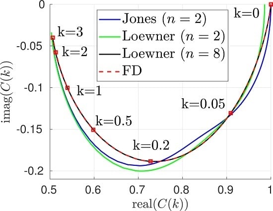
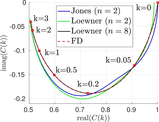
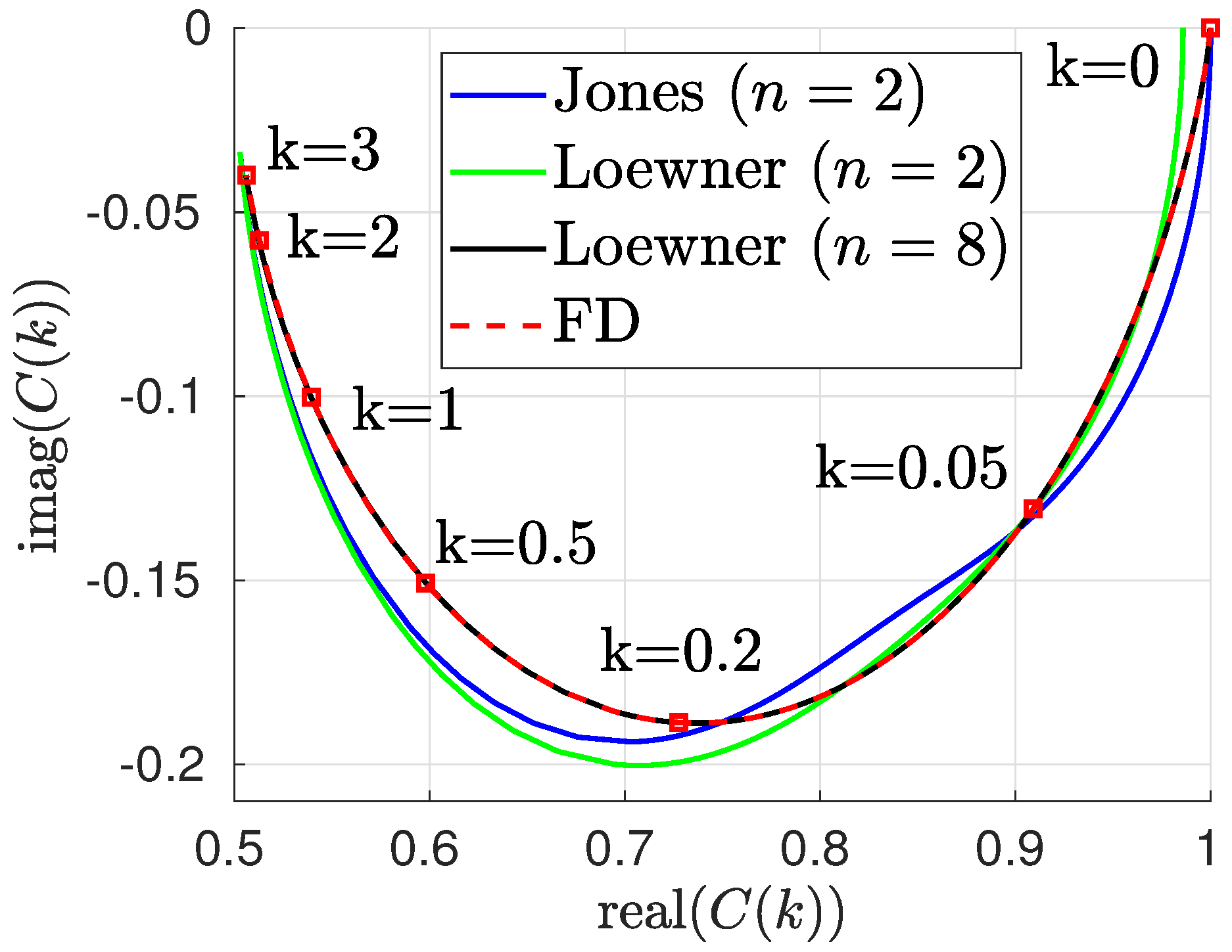
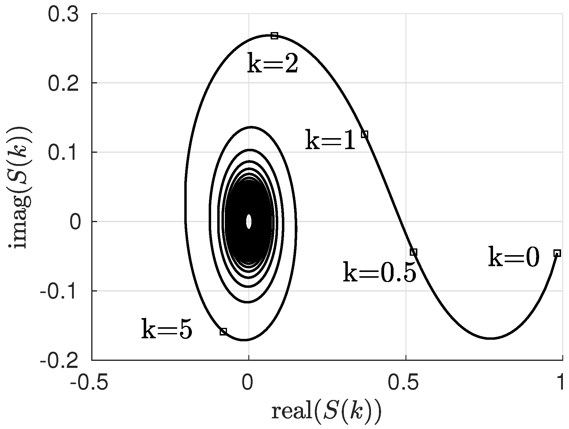
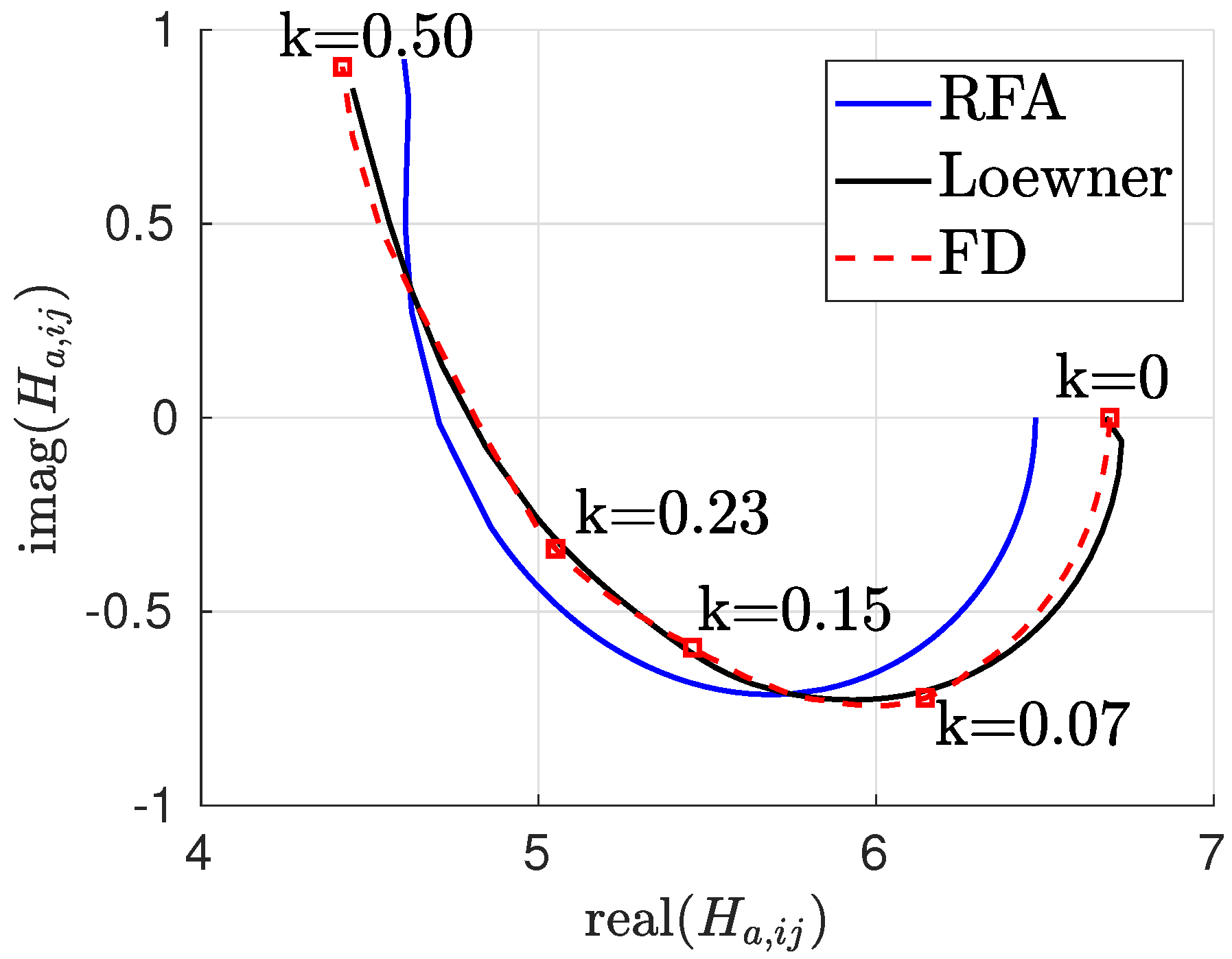
Application to the Theodorsen Function

In the case of bidimensional unsteady incompressible flow, a more general realization can be obtained which is then valid for all values of the parameters involved in Equation (9), namely U , L r e f and a. This is not possible for the more general three-dimensional unsteady compressible flow and an extension of the method presented in Section 2.3 involving a residualization of the aerodynamic matrix transfer function at high frequency values will be applied in Section 3.1.
For a realization of the Theodorsen function, the following strictly proper aerodynamic transfer function is defined:
H c k = C k 1 2 ,
where C k represents the Theodorsen function which depends on the reduced frequency k. Next, the Loewner and shifted Loewner matrices are built and a realization is carried out:
A c = E c r 1 A c r , B c = E c r 1 B c r , C c = E c r 1 C c r , D c = E c r 1 D c r = 0 ,
where the system E c r , A c r , B c r , C c r , D c r is obtained after applying Equations (5) and (7) for a reduction on the number of states and Equation (8) for the suppression of possible unstable poles. The resulting generalized state-space system is:
x ˙ c = A c x c + B c 2 π U 0 U 1 L r e f 1 2 a 0 0 u u ˙ u ¨ c l c m = C c 0 x c + 0 π π U π L r e f U 3 2 a π L r e f U 2 π a L r e f 2 U 2 0 0 0 π L r e f 2 U π L r e f 4 U 2 1 8 a 2 π L r e f 2 2 U 2 u u ˙ u ¨ .
Figure 3 shows different realizations of the Theodorsen function C k in the complex plane for different values of the reduced frequency k. The Jones approximation requires two states. For the Loewner realization, the cases corresponding to a number of states equal to that of Jones ( n = 2 ) and eight are depicted. It becomes clear that the Loewner realization for an increasing number of poles is in agreement with the reference Theodorsen function computed directly in the frequency domain (FD). The number of poles in the Loewner realization is increased by simply modifying the truncation after the SVD decomposition of Equation (6). Note that, unlike for the classical interpolation techniques [42], the Loewner realization does not require the selection of any poles and no iterative optimization is involved. The matrices A c , B c , C c and D c obtained for the case where up to eight states are retained after the SVD decomposition of the Loewner matrix L are provided in Appendix A.

3. Aeroservoelastic System for Loads Analysis

In this section, the tangential interpolation method presented in Section 2.1 is applied to the more general case of an aircraft flying in subsonic compressible flow. Once the aerodynamic system has been obtained in generalized state-space form in Section 3.1, the structural model is also considered and a coupled aeroservoelastic system for dynamic loads prediction including both the MDM and the FSM methods is obtained in Section 3.2.

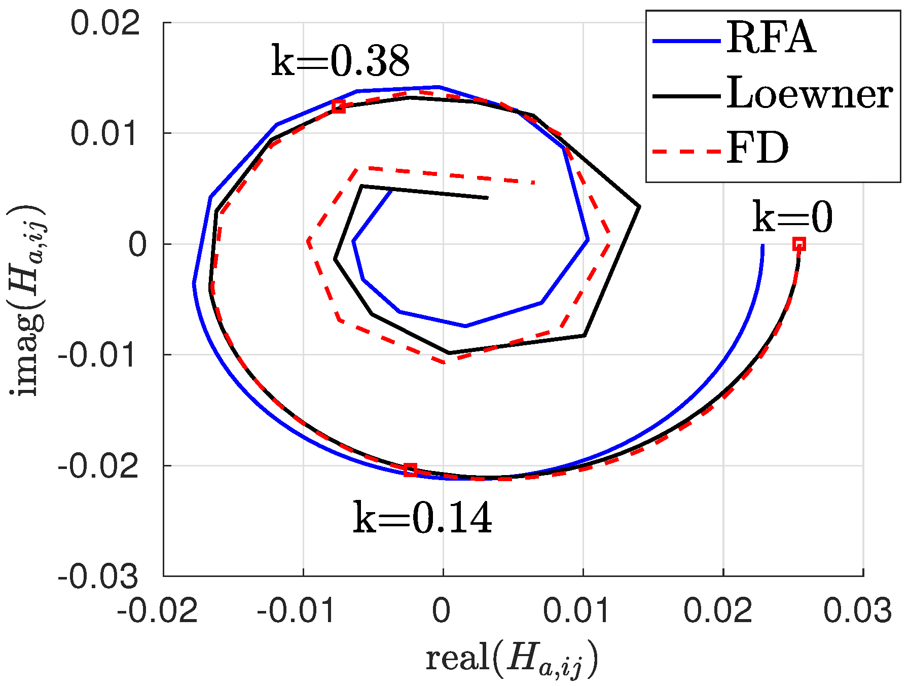
3.1. Generalized Realization of the Aerodynamic System

For the general case of three-dimensional unsteady compressible flow, the transfer function matrix describing the aerodynamic forces cannot be explicitly obtained as for the bidimensional incompressible case, given by Equation (9). A common technique for the computation of the subsonic compressible aerodynamic forces for dynamic loads applications is the doublet lattice method (DLM), which provides the matrix of aerodynamic influence coefficients (AIC) at a set of particular frequencies. Due to the assumption of linear and inviscid flow, the DLM method is not appropriate to describe the transonic flow. In this region, other methods such as the correction of the AIC matrices [43] or linearized computational fluid dynamics (CFD) solvers in the frequency domain can be used [44]. An application including CFD data considering a gust disturbance as input has been shown by Poussot-Vassal et al. [45].
The input of the aerodynamic system is given by the vertical atmospheric disturbance w g at a particular spatial location (the aircraft nose) and a set of generalized coordinates corresponding to the control surfaces u c and the structural modes u h of the aircraft structure (in vacuum) including the rigid-body and flexible modes, as the aeroservoelastic system is reduced by projection into the eigenvalues of the structure (modal truncation). Other directions of the atmospheric disturbance can be included by considering a linear combination of disturbances along three orthogonal axes. Within the usual assumptions for aeroservoelastic modeling, the translational degrees of freedom u t of the aircraft structure do not cause any change in the aerodynamic forces and thus their time derivative is considered here as input to the aerodynamic system. The vector u r f contains the generalized coordinates corresponding to rotational rigid-body motions and to the flexible modes. The aerodynamic forces due to the control surfaces are evaluated by means of a transpiration boundary condition by applying a local variation of the downwash velocity on the related aerodynamic panels but keeping the original panel geometry.
As output y a of the aerodynamic system, the (incremental) local lift and local pitch moment coefficients for the aerodynamic strips defined over the lifting components y a = [ c l T c m T ] T are chosen (see Section 4). With the aerodynamic distribution provided by these coefficients, the cut loads distribution can be recovered over the load reference axis (LRA) by means of the FSM. The aerodynamic transfer function matrix relates the input and output vectors in the frequency domain:
c l ω c m ω = H g ω H t ω H r f ω H c ω w g ω i ω u t ω u r f ω u c ω ,
where H t ω ) = H ω T H / i ω for ω > 0 with T H a matrix selecting the columns from H ω corresponding to the translational degrees of freedom u t . In this way, the singularity caused by the translational motion at frequency zero as described in Section 1 is dealt with systematically.
Within the DLM method, the integrals required to solve the AIC matrices have to be approximated [46]. When considering the aerodynamic transfer function matrix H ω in the limit ω , the polynomial coefficients cannot be obtained from the derivatives of H ω with respect to the circular frequency ω as done in the incompressible case (see Section 2.3). Figure 4 shows a typical element of the transfer function matrix H ω computed numerically for increasing values of the reduced frequency k. Note that the high reduced frequency values shown are beyond the applications of practical interest but would allow for the numerical determination of the non-proper part. It is clear that, for a common DLM aerodynamic model discretization, the method is not able to handle very high frequencies. Indeed, a very high number of panels would be required to properly describe the behaviour at increasing reduced frequencies. Another approach would be to compute the values at very high reduced frequency by means of the piston theory [47]. In this work, a residualization of the transfer function matrix at high frequency values is done by representing it as the sum of a proper and a non-proper part instead.
First, a realization on the aerodynamic transfer function matrix as given in Equation (5) is done. Once the realization E ^ , A ^ , B ^ , C ^ , D ^ has been obtained the eigenvalues of the system are obtained by solving det s E ^ A ^ = 0 . Note that, at this stage, there is no need for an SVD decomposition as this realization is not the final one representing the aerodynamic system. Similarly, no stabilization as described in Section 2.2 is enforced yet. The possible infinite poles due to the non-properness are excluded by setting a tolerance value S . The remaining finite poles are collected in the set S f :
S f = s σ E , A s S .
The column of the aerodynamic transfer function matrix H ω in Equation (14) corresponding to the gust input w g is proper and no split into proper and non-proper part is required. This is coherent with the fact that the Sears function for the gust input problem in the incompressible unsteady case tends to zero for s [48] (see Figure 5). Similarly, no residualization is required when considering the gust disturbance as unique system input [45]. In order to split the proper and non-proper parts for the rest of the columns of the aerodynamic transfer function matrix H ω in a numerical stable way, a least-squares fit of a rational proper transfer function together with a polynomial part is done for each component of the transfer function matrix data (see Equation (16)):
H i j ω = k = 1 N c , i j R i j i ω + p k , i j + P 0 , i j + P 1 , i j i ω P 2 , i j ω 2 ,
where p k , i j , R i j can either be real or come in conjugate pairs, P 0 , i j , P 1 , i j , P 2 , i j R and the sum runs over the number N c , i j of finite poles p k , i j given by Equation (15) and which belong to the set S f , p k , i j S f . The dependence of the finite poles with the indices i j in N c , i j and p k , i j refers to the fact that each component of the transfer function matrix H ω is dealt with separately. Note that, compared to the classical least-squares fit of the RFA technique which uses real coefficients [3,4,14], Equation (16) is able to represent peaks of the aerodynamic transfer functions in the frequency domain which appear in the transonic flow regime [49] by the presence of conjugate pair poles [6]. Additionally, the fit of Equation (16) does not suffer the ill-conditioning present when using an increasing number of real poles. In addition, the use of different poles for each element of the aerodynamic transfer function matrix H ω as done here would lead to a prohibitive number of additional states if the classical approach of a least-squares fit were directly transformed into the time domain [50].
In the next step, the actual data after subtraction of the polynomial non-proper part instead of the strictly proper part of the fit given by the first term of Equation (16) is used. Thus, there is no error introduced in the proper part of the aerodynamic transfer function matrix and the representation of the non-proper part by the polynomial part can be seen as a residualization of the high frequency behaviour of the aerodynamic transfer function matrix H ω , as it is not available from the common aerodynamic solvers in the frequency domain (see Figure 4).
Next, the proper transfer function matrix H a ω is obtained, H a ω = H ω P 0 P 1 i ω + P 2 ω 2 . Similarly as done for the incompressible flow case, now the tangential interpolation method is applied to the proper transfer function matrix H a ω and the realization E a = I , A a = E r 1 A r , B a = E r 1 B r , C a = C r , D a = D r is obtained, where the SVD decomposition and the stabilization enforcement of Section 2.2 are applied afterwards. The matrices B a and D a together with the input vector have to be properly completed to accommodate the non-proper polynomial part (see Equation (17)). The matrices corresponding to the polynomial part have been split in column blocks corresponding to the translational motion ( P 0 t , P 1 t , P 2 t ), rotational and flexible generalized coordinates ( P 1 r f , P 1 r f , P 2 r f ) and control surface deflections ( P 0 c , P 1 c , P 2 c ). The term corresponding to the third time derivative of the translational motion u t is explicitly neglected by setting P 2 t = 0 . The submatrices in [ B a u 1 B a h 2 B a h 1 B a u 2 0 0 0 0 0 0 ] have been defined for convenience in a subsequent reordering of terms:
x a ˙ = A a x a + B a u 1 B a h 2 B a h 1 B a u 2 0 0 0 0 0 0 u a c l c m = C a x a + 0 P 0 t P 0 r f P 0 c P 1 t P 1 r f P 1 c 0 P 2 r f P 2 c u a ,
where u a = [ w g u ˙ t T u r f T u c T u ¨ t T u ˙ r f T u ˙ c T u t T u ¨ r f T u ¨ c T ] T . Dropping the terms corresponding to zero submatrices and reordering, the generalized state-space model for the unsteady aerodynamic loads is:
x ˙ a = A a x a + B a u 1 B a u 2 0 0 w g u c u ˙ c u ¨ c + B a h 1 B a h 2 u r f u t ˙ c l c m = C a x a + 0 P 0 c P 1 c P 2 c w g u c u ˙ c u ¨ c + P 0 r f D a h 2 D a h 3 u r f u ˙ h u ¨ h ,
where u h = [ u t T u r f T ] T and:
D a h 2 = P 0 t P 1 r f D a h 3 = P 1 t P 2 r f .

3.2. Aeroservoelastic System

In this section, the interaction between the aerodynamic and structural parts is considered in order to obtain a complete aeroservoelastic formulation. According to the virtual work principle, the forces transfer from the aerodynamic grid to the structural grid may be done with the corresponding transpose of the spline matrix which transfers the structural deformation to the aerodynamic grid [51]. However, and depending on the spline method for the transfer of forces from the aerodynamic grid to the structural grid, a set of nodal forces which is not smoothly distributed over the airframe but concentrated at particular positions can be obtained with such a transpose matrix. This is not a limitation when computing the generalized aerodynamic forces, but may lead to non realistic cut load distributions when applying the MDM method for the loads recovery. Assuming that the introduced error for not using the transpose of the spline matrix is negligible, the transfer of the aerodynamic forces to the structural grid is done by the summation matrix S g s , which transfers the aerodynamic coefficients acting over the lifting components to the nearest structural grid in the form of dimensional force and moment vectors. In order to obtain the total aerodynamic force acting over the aircraft structure, the resulting aerodynamic forces and moments are multiplied by the dynamic pressure q. The aeroservoelastic problem can be formulated in the time domain as:
M h h u ¨ h + B h h u ˙ h + K h h u h = q ϕ g h T S g s C a x a + 0 P 0 c P 1 c P 2 c w g u c u ˙ c u ¨ c + P 0 r f D a h 2 D a h 3 u r f u ˙ h u ¨ h ,
where M h h , B h h and K h h represent the generalized mass, damping and stiffness matrices, respectively. The matrix ϕ g h contains a number N h (due to modal truncation) of the aircraft structural modes u h (in vacuum) including the rigid-body and flexible modes. As in Section 3.1, the vector u h = [ u t T u r f T ] T represents the total number of generalized coordinates (including rigid-body and structural flexible modes) and u c the control surfaces. The subset u t u h represents the translational rigid-body degrees of freedom and the subset u r f u h the rotational rigid-body degrees of freedom together with the flexible modes. With no generalized stiffness corresponding to the translational degrees of freedom u t , the relation K h h u h = K h r u r f = K h f T f u r f can be used, where the subindex in the submatrix K h f corresponds to the columns related to the subset of generalized coordinates representing the flexible modes u f , obtained with the matrix T f from u r f .
In order to include the translational motion in the system output, the state vector x is augmented, x ^ = [ u t T u r f T u ˙ h T x a T ] T , and the following equation of first order in the time derivatives is obtained:
d d t u t u r f u ˙ h x a = 0 0 T t 0 0 0 T r f 0 0 A h 1 A h 2 A h 3 0 B a h 1 B a h 2 T t A a u t u r f u ˙ h x a + 0 0 0 0 0 0 0 0 0 α 1 T h s P 0 c α 1 T h s P 1 c α 1 T h s P 2 c B a u 1 B a u 2 0 0 w g u c u ˙ c u ¨ c ,
with:
T h s = q ϕ g h T S g s , α = M h h T h s D a h 3 , A h 1 = α 1 k h f T f + T h s P 0 r f , A h 2 = α 1 B h h + T h s D a h 2 , A h 3 = α 1 T h s C a ,
where the matrix T r f selects the non translational degrees of freedom u r f from the generalized coordinates u h (that is, excluding the subset u t corresponding to the translational motion) and the matrix T t selects the translational degrees of freedom from the vector of generalized coordinates u h .
Once the aeroservoelastic system has been written in a generalized state-space form of first order, the loads can be recovered by [52]:
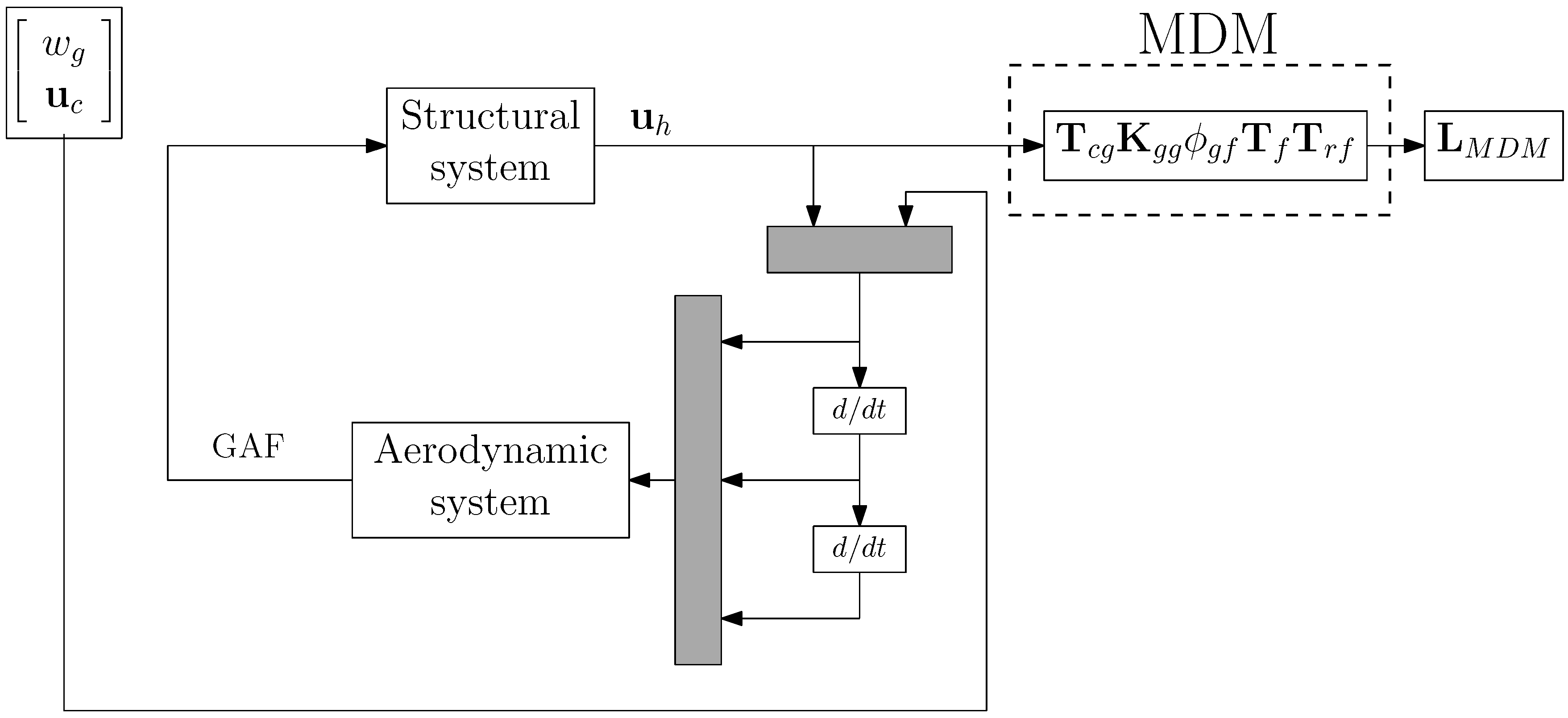
  • Mode displacement method (MDM), where the cut loads are given by:
    L M D M = T c g K g g ϕ g h u h = T c g K g g ϕ g t ϕ g r ϕ g f u t u r u f = T c g K g g ϕ g f u f ,
    where the matrix K g g corresponds to the physical stiffness matrix, ϕ g f includes the columns corresponding to the flexible modes and u f their generalized coordinates. The matrix T c g is a summation matrix which considers the nodal loads adding up to a particular location in order to obtain the resulting (incremental with respect to a steady-state reference) cut loads such as the shear forces together with the bending and torsional moments.
  • Force summation method (FSM), where the cut loads are recovered by the equilibrium of forces:
    L F S M = T c g M g g ϕ g h u ¨ h + q S g s y a ,
    where the matrix M g g represents the physical mass matrix. For the FSM method, not only the generalized aerodynamic forces but also the aerodynamic distribution y a = [ c l T c m T ] T is required.
Both load recovery methods can be included in the output equation of the generalized state-space formulation of first order together with the aircraft response and the aerodynamic distribution:
u t u r f y a L M D M L F S M = I 0 0 0 0 I 0 0 0 P 0 r f + D a h 3 A h 1 D a h 2 + D a h 3 A h 2 C a + D a h 3 A h 3 0 T c g K g g ϕ g f T f 0 0 0 q T c g S g s P 0 r f + β A h 1 q T c g S g s D a h 2 + β A h 2 q T c g S g s C a + β A h 3 u t u r f u ˙ h x a + 0 0 0 0 0 0 0 0 0 P 0 c + D a h 3 α 1 T h s P 0 c P 1 c + D a h 3 α 1 T h s P 1 c P 2 c + D a h 3 α 1 T h s P 2 c 0 0 0 0 0 Γ P 0 c Γ P 1 c Γ P 2 c w g u c u ˙ c u ¨ c ,
where L M D M and L F S M represent the cut loads obtained by the MDM and FSM methods respectively and:
β = T c g M g g ϕ g h + q T c g S g s D a h 3 , Γ = β α 1 T h s + q T c g S g s .
Equations (19) and (20) represent the generalized state-space and output equations for the aeroservoelastic model description in the time domain.
In Figure 6 and Figure 7, the block diagrams corresponding to Equations (19) and (20) for both the MDM and FSM methods are shown respectively. In Figure 7, the matrix T h selects the subset u h from [ u h T u c T ] T .

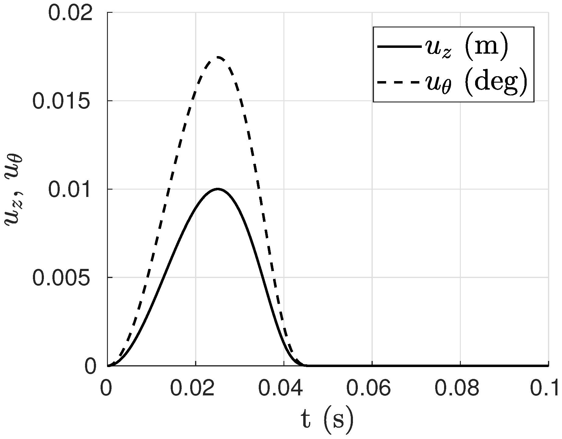
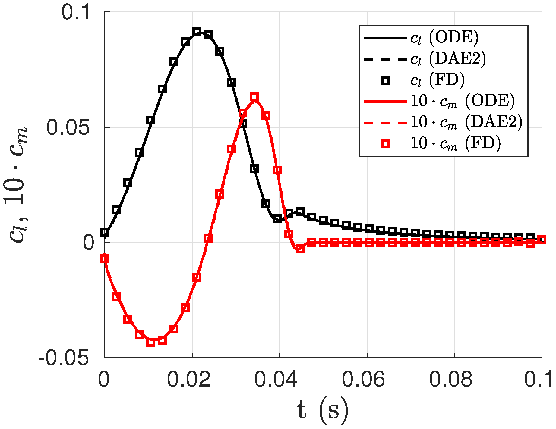
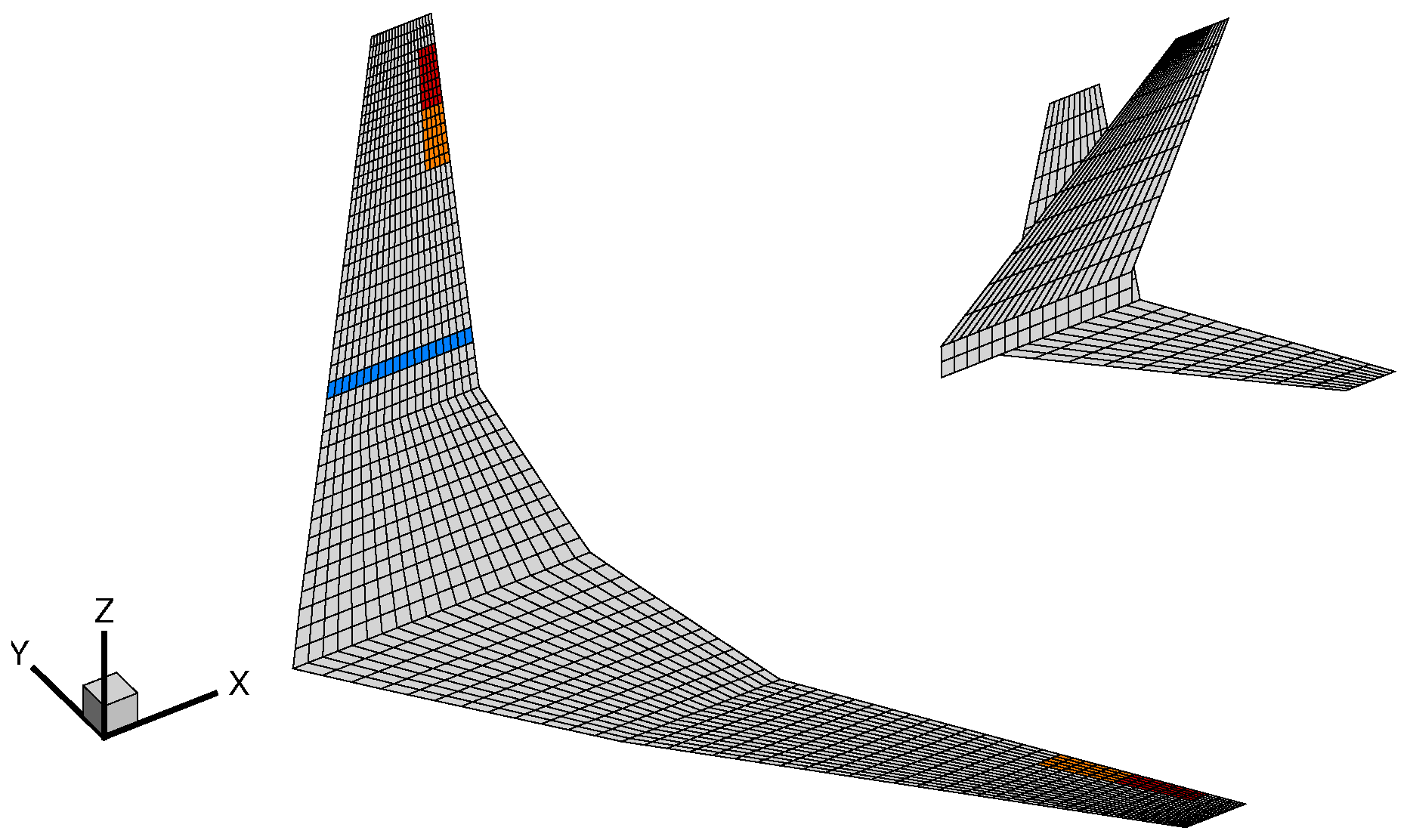
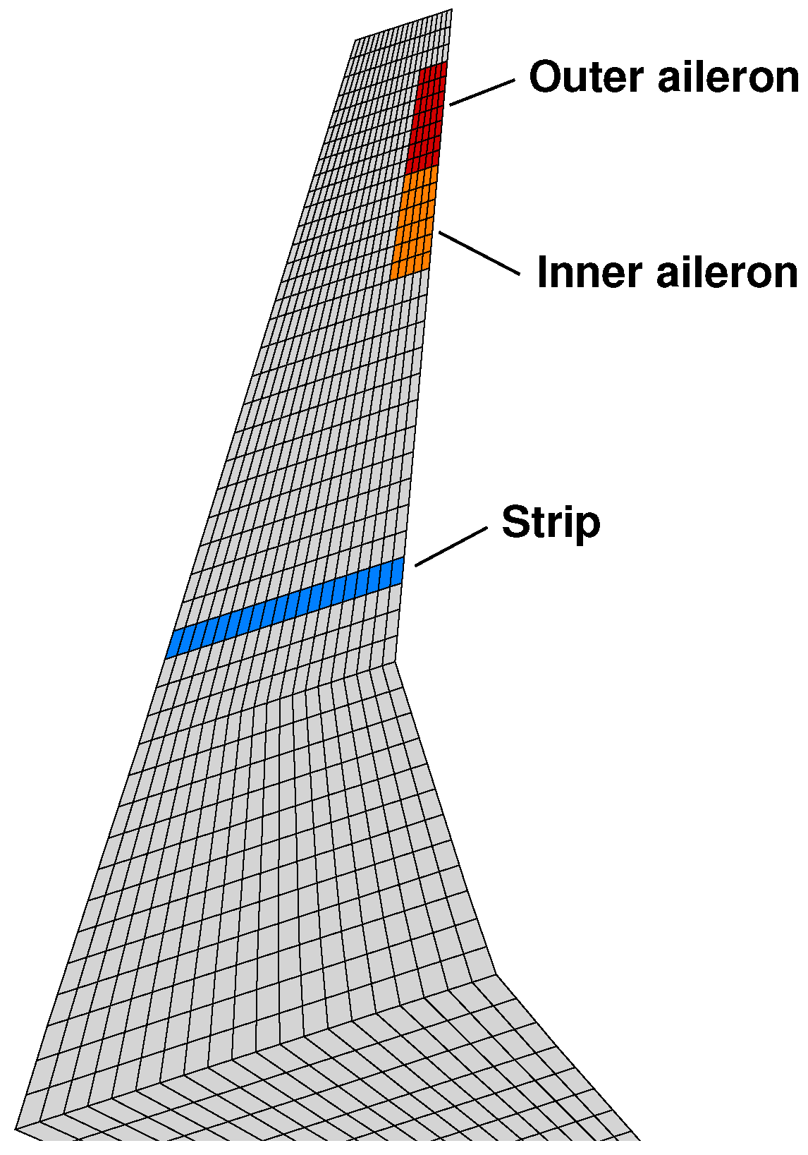
4. Application to the FERMAT Configuration

In this section, the FERMAT model created by Klimmek [53] has been used. The mass case C6 corresponding to a 100% of the fuel mass with a mass equal to the maximum takeoff weight MTOW = 260,000 (kg) and a center of gravity position in the x-direction (see Figure 8 for axes definition) with respect to the aircraft nose position x 0 of x c g x 0 = 33.716 (m) is considered. The spline from the structural model deformation to the aerodynamic grid is carried out by a thin-plate spline (TPS) method [54]. As described in Section 3.2, the TPS method generates a force transfer which may not smoothly distributed over the aircraft structure and thus the summation matrix S g s from Equation (20) is used for the application of the FSM for the cut loads recovery. The cut loads presented in this section are incremental and do not include the loads acting at the 1g or level flight condition.
For the computation of the summation matrix S g s , the lifting surfaces are split up into strips, which are segments of constant width including all panels at a constant y , z position, see Figure 8, where a typical strip aerodynamic element for the right wing component is shown and the panels conforming the control surface panels (ailerons) are highlighted. Neglecting the aerodynamic modeling of the fuselage component, there are a total of 1910 aerodynamic panels representing the complete configuration. The wing semi-span is 29.36 (m). A view of the right wing component is provided in Figure 9. Note that a strip can include panels from the wing component as well as from the aileron if they are topologically connected. The ailerons are taken into account in Section 4.2, where the effect of a gust loads alleviation (GLA) strategy is evaluated using the proposed aeroservoelastic model. In that case, the control surface modes corresponding to the ailerons are modeled with the transpiration approach as described in Section 3.1.
Regarding the dynamic structural model, two symmetric rigid-body modes corresponding to the heave and pitch (around the center of gravity) motion together with the 16 flexible modes ranging in frequencies from 2.03 (Hz) up to 7.30 (Hz) have been taken into account. The structural damping matrix has been set to zero, B h h = 0 . The heave forms the vector u t and the pitch together with the flexible modes form the vector u r f in Equations (19) and (20). The aeroservoelastic system as described in Section 3.2 has been generated for the flightpoint corresponding to a Mach number of M = 0.85 and an altitude h = 7640 (m). The true airspeed is U = 263.147 (m/s) and the reference length for the reduced frequency definition is L r e f = 7.005 (m). The selected set of reduced frequencies for the Loewner realization has been chosen as k = k 1 k 2 k 3 , where k 1 = 0 , , 0.25 with spacing Δ k 1 = 0.005 , k 2 = 0.29 , 0.335 , 0.575 , 0.415 , 0.46 , 0.5 , 0.585 , 0.665 , 0.75 , 0.8350 , 0.915 , 1 and k 3 = 1.165 , 1.335 , 1.5 , 1.665 , 1.835 , 2 , 2.165 , 2.335 , 2.5 , 2.665 , 2.835 , 3 . The interpolation of the precomputed AIC matrices to this set of reduced frequencies is done using a special linear interpolation technique [54]. The tolerance in Equation (15) has been set to S = 10 U / L r e f .
Figure 10 shows the element of the aerodynamic transfer function matrix corresponding to the (incremental) lift coefficient over the strip element at the wing station y = 13.48 (m) shown in Figure 8 and Figure 9 in the complex plane due to a gust disturbance input for the different values of the reduced frequency k. In Figure 11, the pitch motion around the center of gravity is taken as input. For comparison purposes, the results obtained with six real poles applying the classical Roger’s approach (RFA) is also shown [4,5], where the poles p j have been computed as p j = k m a x / j for j = 1 , , 6 with k m a x = 3 . The data labeled as Loewner shows the present method and FD refers to the reference data in the frequency domain. It is clear from Figure 10 and Figure 11 that the present approach shows a better match compared to the Roger’s approach. Because of the finer resolution for the low reduced frequency range in the set of reduced frequencies selected, this better match is more evident in this region, which is of significant importance for aeroelastic applications.

4.1. Open Loop

In this section, the aeroservoelastic model is validated in open loop against the reference model available in the frequency domain. The model is excited by a 1-cosine gust w g t in (m/s) given by (at the aircraft nose) [1]:
w g t = w 0 2 1 c o s π U H t , 0 t 2 H / U , w g t = 0 , t 2 H / U ,
with w 0 the maximum gust amplitude (m/s), U the translational speed (m/s) and H the gust gradient or half length (m). For this application, the gust amplitude has been set to α e q = w 0 / U equivalent to 1 (deg) and the gust gradient to H = 106.68 (m) or H = 350 (ft), the longest according to the regulations [1].
First, the rigid-body modes corresponding to the heave and pitch rotation about the center of gravity have been considered together with the first flexible mode of the structure (in vacuum) representing the symmetrical wing bending and with a natural frequency of 2.03 (Hz), resulting in an aeroservoelastic model in the time domain with a total of 81 states. Even though the ailerons on the wing have been considered in the time-domain realization, they have been set to zero for the open loop validation. The corresponding incremental bending M X and torsional M Y moments obtained by the FSM over the right wing component as predicted by both the aeroservoelastic model in the time domain (labeled as TD) and the reference model in the frequency domain (labeled as FD) are shown in Figure 12 and Figure 13 for the time instants at which the maximum and minimum vales are reached at the wing root location. It can be seen that the aeroservoelastic model with 81 states is able to reproduce the complete time history of the incremental cut loads distribution along the entire wing component.
Next, and in order to show the suitability of the present method for the cut loads recovery by means of the FSM, the effect of considering more flexible modes on the cut loads has been analyzed and a total number of 16 flexible modes ranging from frequencies 2.03 up to 7.30 (Hz) has been retained, obtaining a generalized state-space aeroservoelastic model with 231 states. Figure 14 shows the incremental bending moment M X obtained in time domain (TD) with the resulting aeroservoelastic model with 231 states compared with the reference values computed in the frequency domain (FD) at the time instants where the maximum and minimum values are reached at the wing root. Again, both formulations are in agreement, which is due to the fact that the aerodynamic distribution can be represented in the time domain by the present method as detailed in Section 3.2, as shown in Figure 15 where the incremental lift coefficient distribution c l along the complete wing component is represented at the corresponding time instants.

4.2. Closed Loop

Once the aeroservoelastic model has been validated, the implementation of a simple GLA strategy is shown. An aeroservoelastic model including heave and pitch rigid-body modes, 16 flexible modes together with four ailerons (two inner and two outer) over the wing component has been chosen. As in Section 4.1, the same flightpoint has been selected and the total number of states used for the time-domain realization is 231. A simple proportional law between the gust speed at the aircraft nose and the outer ailerons, which are deployed symmetrically, has been implemented. An additional time delay between the gust speed detection and the aileron command of t d = 0.06 (s) has been taken into account. Thus, the vector u c containing the control surface deflections is given in radian units by:
u c t = 0 P w g t t d 0 P w g t t d T ,
where the constant gain has been set to P = 1 / 50 (s/m) and the zero entries correspond to the inner ailerons. The maximum outer aileron deflection produced with this gain is 5.15 (deg). It is clear from Figure 16 that the maximum value of the incremental wing root bending moment M X can be reduced in 19.01% at the expense of increasing the incremental torsional moment M Y in 14.01% (see Figure 17). Furthermore, the proposed aeroservoelastic model enables the evaluation of the effects of the applied GLA strategy on the cut loads over the complete aircraft structure.

5. Conclusions

In this work, an aeroservoelastic model for the prediction of the aeroelastic response together with the dynamic loads over the complete aircraft structure has been presented. It represents an interpolation instead of an approximation of the reference model in the frequency domain. The distributed aerodynamic forces created by the gust disturbance and induced by the aircraft motion can be obtained in the time domain and coupled with the structural model to obtain an aeroservoelastic state-space model of first order which includes the effect of control surfaces deflection. The force summation method can be used for the loads recovery, taking advantage of its superior convergence with the number of generalized coordinates in comparison with the mode displacement method.
The presented aeroservoelastic model can be used for further implementation of GLA strategies, including multivariable control design. As an application, a simple GLA logic with a proportional feedback closed loop architecture has been implemented to demonstrate the suitability of the present approach for aeroservoelastic design.
Related future work includes:
  • Different GLA control law strategies. Within the presented method, the complete aerodynamic distribution together with the cut loads and combinations thereof can be chosen as objective functions.
  • Consideration of different aerodynamic theories in the frequency domain which are appropriate for the transonic flow, such as the correction of the AIC matrices or linearized CFD solvers in the frequency domain. In particular, the piston theory as limit of the DLM method for high reduced frequency values may also be considered. In this case, the residualization could be eliminated by substracting the values predicted by the piston theory from the aerodynamic transfer function matrix.
  • Inclusion of parametric generalized state-space aeroservoelastic models as an alternative to the classical gain scheduling approach.
  • Extension to a nonlinear generalized state-space formulation for nonlinear aeroservoelastic systems. In this case, the Loewner framework in connection with a functional or Volterra series expansion theory can be followed.

Author Contributions

D.Q. developed and implemented the aeroservoelastic formulation and wrote the manuscript, P.V. and C.P.-V. implemented the Loewner framework algorithms and reviewed the manuscript.

Funding

This work has been funded within the frame of the Joint Technology Initiative JTI Clean Sky 2, AIRFRAME Integrated Technology Demonstrator platform “AIRFRAME ITD” (contract N. CSJU-CS2-GAM-AIR-2015-15-01 Annex 1, Issue B04, 2 October 2015) being part of the Horizon 2020 research and Innovation framework programme of the European Commission.

Conflicts of Interest

The authors declare no conflict of interest.

Appendix A. Theodorsen Function Realization

Here, the matrices obtained after applying the Loewner realization given by Equation (5) to the Theodorsen function, followed by an SVD truncation retaining eight states, see Equation (7), and a projection into the R H space in order to avoid the possible appearance of unstable poles, see Equation (8), are given:
A c = 70.2475 15.2084 4.3860 1.5667 0.6656 0.2916 0.1426 0.0659 127.6550 60.8706 23.0820 8.5669 3.5625 1.5389 0.7418 0.3415 168.3215 105.6100 59.3595 26.9511 11.5870 4.9825 2.3544 1.0755 225.3710 146.1488 100.3562 60.3945 30.6229 13.8770 6.5170 2.9615 315.4916 200.8967 143.6691 101.8372 64.7094 34.1741 16.5753 7.5699 451.2802 282.2752 200.3830 148.7585 109.8055 72.2007 40.6074 19.7354 681.3672 420.8463 294.1354 217.1403 167.1839 127.0703 87.6431 50.0344 967.5574 594.0846 411.6020 301.1651 232.6729 187.3735 150.9202 108.2737 ,
B c = 5.7098 8.1427 11.6790 16.7748 24.4703 35.7673 54.6494 78.0051 ,
C c = 5.7516 0.9726 0.3074 0.1170 0.0521 0.0233 0.0115 0.0054 .
These matrices can then be used in Equation (13) to obtain a complete representation of the unsteady bidimensional incompressible flow over an airfoil with heave and pitch degrees of freedom. For an approximation with a number of states lower than eight, n < 8 , the first n rows and columns of the matrix A c above should be taken. Similarly, the first n entries of the vectors B c and C c should be considered.

References

  1. European Aviation Safety Agency. Certification Specifications and Acceptable Means of Compliance for Large Aeroplanes; Technical Report CS-25, Amendment 16; European Aviation Safety Agency: Cologne, Germany, 2015. [Google Scholar]
  2. Federal Aviation Regulations Part 25: Airworthiness Standards: Transport Category Airplanes. Web Resource for Research. 2015. Available online: http://www.risingup.com/fars/info/25-index.shtml (accessed on 15 March 2012).
  3. Eversman, W.; Tewari, A. Consistent rational-function approximation for unsteady aerodynamics. J. Aircr. 1991, 28, 545–552. [Google Scholar] [CrossRef]
  4. Roger, K.L. Airplane Math Modeling Methods for Active Control Design. In Proceedings of the 44th AGARD Structures and Material Panel (AGARD-CP-228), Lisbon, Portugal, 21 April 1977. [Google Scholar]
  5. Abel, I. An Analytical Technique for Predicting the Characteristics of a Flexible Wing Equipped with an Active Flutter-Suppression System and Comparison with Wind-Tunnel Data; Technical Report, NASA Technical Paper 1367; NASA Langley Research Center: Hampton, VA, USA, 1979.
  6. Gustavsen, B.; Semlyen, A. Rational approximation of frequency domain responses by vector fitting. IEEE Trans. Power Deliv. 1999, 14, 1052–1061. [Google Scholar] [CrossRef]
  7. Gustavsen, B.; Semlyen, A. A robust approach for system identification in the frequency domain. IEEE Trans. Power Deliv. 2004, 19, 1167–1173. [Google Scholar] [CrossRef]
  8. Karpel, M.; Moulin, B.; Chen, P. Dynamic response of aeroservoelastic systems to gust excitation. J. Aircr. 2005, 42, 1264–1272. [Google Scholar] [CrossRef]
  9. Mor, M.; Livne, E. Sensitivities and approximations for aeroservoelastic shape optimization with gust response constraints. J. Aircr. 2006, 43, 1516–1527. [Google Scholar] [CrossRef]
  10. Pusch, M.; Knoblach, A.; Kier, T. Integrated optimization of ailerons for active gust load alleviation. In Proceedings of the International Forum on Aeroelasticity and Structural Dynamics (IFASD), St. Petersburg, Russia, 28 June–2 July 2015. [Google Scholar]
  11. Castrichini, A.; Cooper, J.; Benoit, T.; Lemmens, Y. Gust and Ground Loads Integration for Aircraft Landing Loads Prediction. In Proceedings of the 58th AIAA/ASCE/AHS/ASC Structures, Structural Dynamics, and Materials Conference, Grapevine, TX, USA, 9–13 January 2017. [Google Scholar]
  12. Dunn, H. An Analytical Technique for Approximating Unsteady Aerodynamics in the Time Domain; Technical Report, NASA Technical Paper 1738; NASA Langley Research Center: Hampton, VA, USA, 1980.
  13. Tiffany, S.; Adams, W., Jr. Nonlinear programming extensions to rational function approximations of unsteady aerodynamics. In Proceedings of the 28th Structures, Structural Dynamics and Materials Conference, Monterey, CA, USA, 6–8 April 1987. [Google Scholar]
  14. Karpel, M. Design for Active Flutter Suppression and Gust Alleviation Using State-Space Aeroelastic Modeling. J. Aircr. 1982, 19, 221–227. [Google Scholar] [CrossRef]
  15. Pototzky, A.; Perry, B., III. New and existing techniques for dynamic loads analyses of flexible airplanes. J. Aircr. 1986, 23, 340–347. [Google Scholar] [CrossRef]
  16. Karpel, M.; Presente, E. Structural dynamic loads in response to impulsive excitation. J. Aircr. 1995, 32, 853–861. [Google Scholar] [CrossRef]
  17. Liu, X.; Sun, Q.; Cooper, J. LQG based model predictive control for gust load alleviation. Aerosp. Sci. Technol. 2017, 71, 499–509. [Google Scholar] [CrossRef]
  18. Juang, J.; Pappa, R. An Eigensystem Realization Algorithm for Modal Parameter Identification and Model Reduction. J. Guid. Control Dyn. 1985, 8, 620–627. [Google Scholar] [CrossRef]
  19. Silva, W.; Bartels, R. Development of reduced-order models for aeroelastic analysis and flutter prediction using the CFL3Dv6.0 code. J. Fluids Struct. 2004, 19, 729–745. [Google Scholar] [CrossRef]
  20. Gaitonde, A.; Jones, D. Reduced order state-space models from the pulse responses of a linearized CFD scheme. Int. J. Numer. Methods Fluids 2003, 42, 581–606. [Google Scholar] [CrossRef]
  21. Ma, Z.; Ahuja, S.; Rowley, C. Reduced-order models for control of fluids using the eigensystem realization algorithm. Theor. Comput. Fluid Dyn. 2011, 25, 233–247. [Google Scholar] [CrossRef]
  22. Rowley, C. Model reduction for fluids using balanced proper orthogonal decomposition. Int. J. Bifurc. Chaos 2005, 15, 997–1013. [Google Scholar] [CrossRef]
  23. Kramer, B.; Gugercin, S. Tangential interpolation-based eigensystem realization algorithm for MIMO systems. Math. Comput. Model. Dyn. Syst. 2016, 22, 282–306. [Google Scholar] [CrossRef]
  24. Antoulas, A. Approximation of Large-Scale Dynamical Systems; SIAM: Philadelphia, PA, USA, 2005; Volume 6. [Google Scholar]
  25. Mayo, A.; Antoulas, A. A framework for the solution of the generalized realization problem. Linear Algebra Its Appl. 2007, 425, 634–662. [Google Scholar] [CrossRef] [Green Version]
  26. Karpel, M.; Shousterman, A.; Mindelis, Y. Rigid-Body Issues in FFT-Based Dynamic Loads Analysis with Aeroservoelastic Nonlinearities. In Proceedings of the 53rd AIAA/ASME/ASCE/AHS/ASC Structures, Structural Dynamics and Materials Conference, Honolulu, HI, USA, 23–26 April 2012. [Google Scholar] [CrossRef]
  27. Moulin, B.; Karpel, M. Gust Loads Alleviation Using Special Control Surfaces. J. Aircr. 2007, 44, 17–25. [Google Scholar] [CrossRef]
  28. Sokolov, V. Contributions to the Minimal Realization Problem for Descriptor Systems. Ph.D. Thesis, Technical University Chemnitz, Chemnitz, Germany, 2006. [Google Scholar]
  29. Lefteriu, S.; Antoulas, A. A new approach to modeling multiport systems from frequency-domain data. IEEE Trans. Comput.-Aided Des. Integr. Circuits Syst. 2010, 29, 14–27. [Google Scholar] [CrossRef]
  30. Köhler, M. On the closest stable descriptor system in the respective spaces RH2 and RH. Linear Algebra Appl. 2014, 443, 34–49. [Google Scholar] [CrossRef]
  31. Theodorsen, T. General Theory of Aerodynamic Instability and the Mechanism of Flutter; NACA Technical Report 496; National Advisory Committee for Aeronautics, Langley Aeronautical Lab.: Langley Field, VA, USA, 1935.
  32. Brunton, S. Unsteady Aerodynamic Models for Agile Flight at Low Reynolds Numbers. Ph.D. Thesis, Princeton University, Princeton, NJ, USA, 2012. [Google Scholar]
  33. Peters, D. Two-dimensional incompressible unsteady airfoil theory—An overview. J. Fluids Struct. 2008, 24, 295–312. [Google Scholar] [CrossRef]
  34. Hodges, D.; Pierce, G. Introduction to Structural Dynamics and Aeroelasticity, 2nd ed.; Cambridge Aerospace Series; Cambridge University Press: Cambridge, UK, 2011. [Google Scholar] [CrossRef]
  35. Gear, C. An introduction to numerical methods for ODEs and DAEs. In Real-Time Integration Methods for Mechanical System Simulation; Springer: Berlin/Heidelberg, Germany, 1991; pp. 115–126. [Google Scholar] [CrossRef]
  36. Roberts, A. Differential Algebraic Equation Solvers. 1998. Available online: https://de.mathworks.com/matlabcentral/fileexchange/28-differential-algebraic-equation-solvers (accessed on 6 April 2018).
  37. Petzold, L. Description of DASSL: A Differential/Algebraic System Solver; Technical Report; Sandia National Labs.: Livermore, CA, USA, 1982.
  38. Mazelsky, B. On the Noncirculatory Flow about a Two-Dimensional Airfoil at Subsonic Speeds. J. Aeronaut. Sci. 1952, 19, 848–849. [Google Scholar] [CrossRef]
  39. Miles, J. On virtual mass and transient motion in subsonic compressible flow. Q. J. Mech. Appl. Math. 1951, 4, 388–400. [Google Scholar] [CrossRef]
  40. Vepa, R. Finite State Modeling of Aeroelastic Systems; Technical Report; NASA Contractor Report 2779; NASA: Washington, DC, USA, 1977.
  41. Fonte, F.; Ricci, S.; Mantegazza, P. Gust load alleviation for a regional aircraft through a static output feedback. J. Aircr. 2015, 52, 1559–1574. [Google Scholar] [CrossRef]
  42. Eversman, W.; Tewari, A. Modified exponential series approximation for the Theodorsen function. J. Aircr. 1991, 28, 553–557. [Google Scholar] [CrossRef]
  43. Quero, D. An Aeroelastic Reduced Order Model for Dynamic Response Prediction to Gust Encounters. Ph.D. Thesis, Technical University of Berlin, Berlin, Germany, 2017. [Google Scholar] [CrossRef]
  44. Kaiser, C.; Freidewald, D.; Quero, D.; Nitzsche, J. Aeroelastic Gust Load Prediction based on Time-Linearized RANS Solutions. In Proceedings of the Deutscher Luft- und Raumfahrtkongress, Braunschweig, Germany, 13–15 September 2016. [Google Scholar]
  45. Poussot-Vassal, C.; Quero, D.; Vuillemin, P. Data-driven approximation of a high fidelity gust-oriented flexible aircraft dynamical model. In Proceedings of the 9th International Conference on Mathematical Modelling, Vienna, Austria, 21–23 February 2018. [Google Scholar] [CrossRef]
  46. Blair, M. A Compilation of the Mathematics Leading to the Doublet Lattice Method; Technical Report; Air Force Wright Laboratory: Dayton, OH, USA, 1992. [Google Scholar]
  47. Rodden, W.; Farkas, W.; Heathera, M.; Kliszewski, A. Aerodynamic Influence Coefficients From Piston Theory: Analytical Development and Computational Procedure; TDR-169-(3230-11)-TN-2; Aerospace Corp.: El Segundo, CA, USA, 1962. [Google Scholar]
  48. Sears, W. A Systematic Presentation of the Theory of Thin Airfoils in Non-Uniform Motion. Ph.D. Thesis, California Institute of Technology, Pasadena, CA, USA, 1938. [Google Scholar]
  49. Friedewald, D.; Thormann, R.; Kaiser, C.; Nitzsche, J. Quasi-steady doublet-lattice correction for aerodynamic gust response prediction in attached and separated transonic flow. CEAS Aeronaut. J. 2018, 9, 53–66. [Google Scholar] [CrossRef]
  50. Smith, T.A.; Hakanson, J.; Nair, S.; Yurkovich, R. State-space model generation for flexible aircraft. J. Aircr. 2004, 41, 1473–1481. [Google Scholar] [CrossRef]
  51. Beckert, A.; Wendland, H. Multivariate interpolation for fluid-structure-interaction problems using radial basis functions. Aerosp. Sci. Technol. 2001, 5, 125–134. [Google Scholar] [CrossRef] [Green Version]
  52. Reschke, C. Integrated Flight Loads Modelling and Analysis for Flexible Transport Aircraft. Ph.D. Thesis, University of Stuttgart, Stuttgart, Germany, 2006. [Google Scholar]
  53. Klimmek, T. Parametric set-up of a structural model for FERMAT configuration aeroelastic and loads analysis. J. Aeroelasticity Struct. Dyn. 2014, 3. [Google Scholar] [CrossRef]
  54. MSC Software Corporation (Ed.) Aeroelastic Analysis User’s Guide, version 68; MSC Software Corporation: Santa Ana, CA, USA, 2004. [Google Scholar]
Figure 1. Heave u z and pitch u α pitch input.
Aerospace 06 00009 g001
Figure 2. Lift and pitch moment coefficients ( c l , c m ) as predicted by the system of ordinary differential equations (ODE) and the system of differential algebraic equations (DAE) of index 2. Reference results obtained in the frequency domain (FD) are also shown.
Aerospace 06 00009 g002
Figure 3. Theodorsen function in the complex plane and corresponding Jones approximation and Loewner realizations.
Aerospace 06 00009 g003
Figure 4. Typical element of the aerodynamic matrix transfer function (magnitude) against the reduced frequency.
Aerospace 06 00009 g004
Figure 5. Sears function S k in the complex plane.
Aerospace 06 00009 g005
Figure 6. Mode displacement method (MDM).
Aerospace 06 00009 g006
Figure 7. Force summation method (FSM).
Aerospace 06 00009 g007
Figure 8. Typical strip element (blue) and control surfaces (red and orange) for the flutter reduced order assessment (FERMAT) configuration.
Aerospace 06 00009 g008
Figure 9. Typical strip element (blue) and control surfaces (red and orange) for the FERMAT configuration (view of the right wing component).
Aerospace 06 00009 g009
Figure 10. Element of the transfer function matrix from the gust input to the lift coefficient for the strip at the wing station y = 13.48 (m).
Aerospace 06 00009 g010
Figure 11. Element of the transfer function matrix from the pitch input to the lift coefficient for the strip at the wing station y = 13.48 (m).
Aerospace 06 00009 g011
Figure 12. Incremental bending moment M X over the right wing component at different time instants for M = 0.85 , h = 7640 (m), H = 106.68 (m) and α e q = 1 (deg). Two rigid-body modes and one flexible mode considered. Results obtained by the FSM with the generalized state-space model in the time domain (TD) of 81 states compared to the reference model in the frequency domain (FD).
Aerospace 06 00009 g012
Figure 13. Incremental torsional moment M Y over the right wing component at different time instants for M = 0.85 , h = 7640 (m), H = 106.68 (m) and α e q = 1 (deg). Two rigid-body modes and one flexible mode considered. Results obtained by the FSM with the generalized state-space model in the time domain (TD) of 81 states compared to the reference model in the frequency domain (FD).
Aerospace 06 00009 g013
Figure 14. Incremental bending moment M X over the right wing component at different time instants for M = 0.85 , h = 7640 (m), H = 106.68 (m) and α e q = 1 (deg). Two rigid-body modes and 16 flexible modes considered. Results obtained by the FSM with the generalized state-space model in the time domain (TD) of 231 states compared to the reference model in the frequency domain (FD).
Aerospace 06 00009 g014
Figure 15. Incremental lift coefficient c l over the complete wing component at different time instants for M = 0.85 , h = 7640 (m), H = 106.68 (m) and α e q = 1 (deg). Two rigid-body modes and 16 flexible modes considered. Results obtained with the generalized state-space model in the time domain (TD) of 231 states compared to the reference model in the frequency domain (FD).
Aerospace 06 00009 g015
Figure 16. Time history of the incremental bending moment M X at the wing root with and without gust load alleviation (GLA) strategy.
Aerospace 06 00009 g016
Figure 17. Time history of the incremental torsional moment M Y at the wing root with and without GLA strategy.
Aerospace 06 00009 g017

