A Multi-Fidelity Uncertainty Propagation Model for Multi-Dimensional Correlated Flow Field Responses

Abstract

Given the randomness inherent in fluid dynamics problems and limitations in human cognition, Computational Fluid Dynamics (CFD) modeling and simulation are afflicted with non-negligible uncertainties, casting doubts on the credibility of CFD. Scientifically and rigorously quantifying the uncertainty of CFD is paramount for assessing its credibility and informing engineering decisions. In order to quantify the uncertainty of multidimensional flow field responses stemming from uncertain model parameters, this paper proposes a method based on Gappy Proper Orthogonal Decomposition (POD) for supplementing high-fidelity flow field data within a framework that leverages POD and surrogate models. This approach enables the generation of corresponding high-fidelity flow fields from low-fidelity ones, significantly reducing the cost of high-fidelity flow field computation in uncertainty propagation modeling. Through an analysis of the impact of uncertainty in the coefficients of the Spalart–Allmaras (SA) turbulence model on the distribution of wall friction coefficients for the NACA0012 airfoil and pressure coefficients for the M6 wing, the proposed multi-fidelity modeling approach is demonstrated to offer significant advancements in both accuracy and efficiency compared to single-fidelity methods, providing a robust and efficient prediction model for large-scale random sampling.

1. Introduction

With the continuous advancements in mathematical models, numerical algorithms, mesh technologies, and high-performance computing, CFD has emerged as a pivotal tool in numerous critical engineering fields, including aerospace, energy and power, transportation, and beyond. Nevertheless, the credibility of CFD has been a subject of contention due to the non-negligible uncertainties inherent in its models, parameters, and numerical solutions [1]. A comprehensive and rigorous quantification of these uncertainties is imperative for assessing and enhancing the credibility of CFD.

Parameters serve as a significant source of uncertainty in CFD. Due to limitations in human cognition or the inherent randomness in fluid problems, model parameters or inflow conditions may possess a certain degree of uncertainty. To quantify the uncertainty introduced by parameters, scholars have developed various methods, such as Monte Carlo-type random sampling and polynomial chaos [2]. While Monte Carlo-type methods are straightforward, they require a large number of samples to obtain stable and accurate statistical results. Polynomial chaos methods rely on orthogonal polynomial expansions, with coefficients obtained through numerical integration or regression analysis. However, as the dimension of input parameters and the order of expansion increase, the number of samples required for polynomial chaos methods grows drastically, leading to the “curse of dimensionality”. For complex engineering problems, each CFD simulation is computationally expensive, limiting the practical application of these methods due to high computational costs. In recent years, scholars have attempted to introduce machine learning algorithms into the field of numerical simulation uncertainty quantification, using surrogate models to replace complex simulation systems and combining experimental design methods to reduce the demand for sample data [3,4,5,6]. This represents a successful amalgamation of intelligent learning algorithms and uncertainty quantification (UQ) research.

The accuracy of using surrogate models for UQ analysis heavily relies on the accuracy of the surrogate model itself, while the efficiency is determined by the time taken to train and run the surrogate model. Factors such as the size and quality of the training data, feature selection, and the design and training of machine learning algorithms can all affect the accuracy and efficiency of surrogate models. To further improve these aspects, scholars have proposed multi-fidelity modeling methods that leverage the respective strengths of high/low-fidelity analysis models. These methods use a larger number of low-fidelity samples to reduce computational complexity, while also incorporating a smaller number of high-fidelity samples to ensure the predictive performance of the multi-fidelity approximate model. This effectively balances the trade-off between the predictive performance of the approximate model and modeling costs. Commonly used multi-fidelity models include co-Kriging models [7,8,9] and multi-fidelity neural networks [10,11], which have demonstrated great potential in complex equipment optimization design and provide new ideas for quantifying parameter uncertainty propagation in CFD.

However, most existing multi-fidelity models are only applicable to single-output scenarios. In CFD, the outputs of interest not only include individual variables but may also involve flow field variables that vary with time or space, such as wall pressure coefficient distributions and the unsteady aerodynamic forces of aircraft. There may exist potential correlations among flow field variables at different locations or times, and the dimensionality of the output can reach hundreds or even thousands. Moreover, the response dimensions under different fidelities may differ, such as flow fields under different grid scales or unsteady aerodynamic forces under different time steps. Developing multi-fidelity models suitable for uncertainty propagation modeling remains a challenging problem that urgently needs to be solved.

To address the uncertainty quantification problem in multidimensional and correlated flow fields, we developed a modeling method for uncertainty propagation based on Proper Orthogonal Decomposition (POD) and surrogate models. By employing POD, several key basis functions representing flow structures are identified, reducing the multidimensional flow field responses, which span hundreds or even thousands of dimensions, to a reduced-dimensional representation of approximately ten dimensions, which is composed of basis function coefficients. Subsequently, a prediction model is established between the uncertain model parameters and the basis function coefficients. Since POD provides a bidirectional representation between flow field variables and basis function coefficients, it enables the prediction of flow fields under arbitrary model parameters, providing a reliable prediction model for Monte Carlo and other random sampling methods. However, previous studies have primarily relied on data from a single fidelity level. To fully leverage CFD calculation data from different fidelities, this paper presents a high-fidelity data completion method based on Gappy POD, further reducing the sample requirements of existing methods for high-fidelity data.

The paper is organized as follows. The second section introduces the implementation framework and main theoretical methods of the entire approach, including POD, Gappy POD, and Kriging models. The third section presents the cases studied: the low-speed flow around an NACA0012 airfoil and the transonic flow around an M6 wing. The fourth section contains the analysis results of the cases, including the prediction accuracy analysis of Gappy POD and the entire method, the statistical information of the flow field, and the parameter sensitivity results. Finally, the conclusion and future directions for further research are discussed.

2. Uncertainty Propagation Model Framework and Key Algorithms

In the field of CFD, using different grid densities, time step sizes, etc., can generate computational data of varying fidelities. To reduce the overall modeling cost of the uncertainty propagation model, this study adopts a multi-fidelity modeling framework that combines flow field reduction and surrogate modeling. The overall implementation process is shown in Figure 1. The left part of the figure represents the main algorithms used in each stage, and the right part is the model training process. Below, we focus on introducing the model training process.

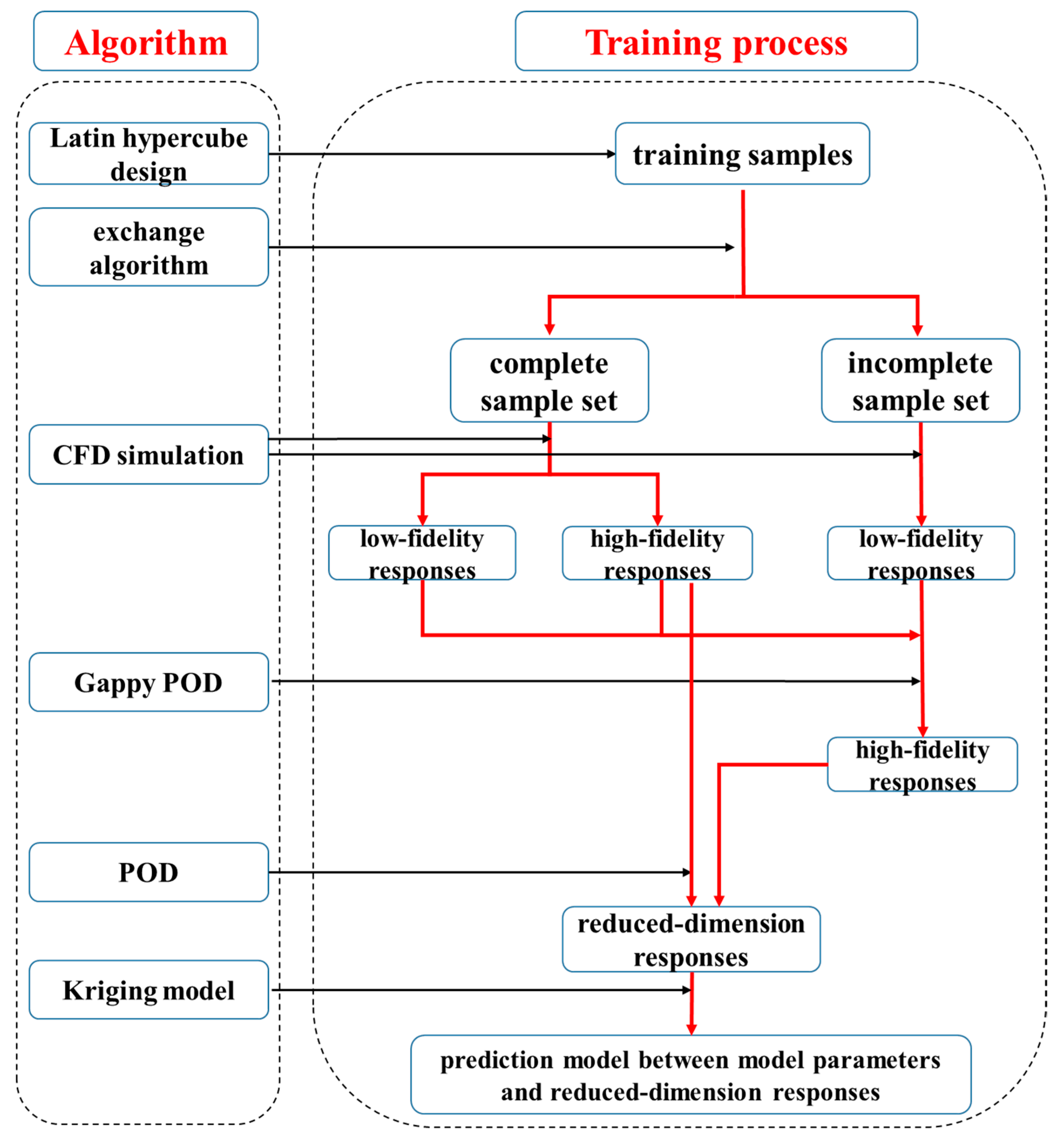
2.1. Model Training Process

The entire model training process can be implemented using the following six steps:

(1)

In the input parameter space, Latin hypercube sampling is employed to generate the inputs for the n_train training samples.

(2)

Based on the inputs of the training samples, the exchange algorithm [12] based on the Morris–Mitchell criterion [13] is used to divide the n_train training samples into two parts: M complete samples and n_train m incomplete samples.

(3)

For the M complete samples, their corresponding high- and low-fidelity outputs are obtained through CFD calculations. For the n_train m incomplete samples, only their corresponding low-fidelity outputs are obtained through CFD calculations, while their high-fidelity outputs are considered unknown.

Of course, we also obtain the high-fidelity outputs of n_train m incomplete samples through CFD calculations. However, these data are not used for model training but only for testing the prediction ability of the Gappy POD method described below.

(4)

Using the Gappy POD method [14,15], the high-fidelity outputs of n_train m incomplete samples are predicted. At this point, the high-fidelity output results for all n_train training samples can be obtained. The low-fidelity output results of these samples will no longer be used hereinafter.

(5)

POD [16,17] is performed on the high-fidelity outputs of the n_train training samples to obtain an orthogonal basis function space. Through projection, the basis function coefficients for each training sample are obtained, which are considered the new outputs.

(6)

Based on the n_train training samples, a Kriging model [18,19] is constructed between the input parameters and the basis function coefficients. Since the orthogonal basis functions obtained through POD are mutually orthogonal, an individual model can be constructed for each basis function coefficient. When given new input parameters, the corresponding basis function coefficients can be predicted based on the models, and the complete flow field response can be reconstructed using the bidirectional expression of POD.

2.2. Model Testing Process

In the input parameter space, Latin hypercube sampling is again employed to obtain the inputs for the n_test training samples. The CFD program is run to obtain high-fidelity sample outputs, which are used to evaluate the prediction accuracy of the overall model.

2.3. Exchange Algorithm

After obtaining n_train training samples, we select M samples from them to perform complete high- and low-fidelity simulations using CFD. Theoretically, the M samples should ideally have good space-filling property in the parameter space. Here, the criterion proposed by Morris and Mitchell [13] is adopted to measure the space-filling property of the sample set, i.e., a good space-filling design should maximize the minimum inter-site distance:

$$\max :\underset{1\le i<j\le n}{\min }{d}_{ij}$$

where d_ij is the Euclidean distance between the two samples x_i and x_j, and n represents the number of samples in the sample set.

To achieve a better space-filling property, the exchange algorithm proposed by Cook and Nachtsheim [12] is employed. Specifically, M samples are randomly selected from the training sample set as the complete sample set ${\mathit{X}}_e$, with the remaining samples forming the incomplete sample set ${\mathit{X}}_r$. The minimum inter-site distance of ${\mathit{X}}_e$ is calculated. We then exchange the first sample in ${\mathit{X}}_e$ (denoted as ${\mathit{x}}_e^{(1)}$) with each of the samples in ${\mathit{X}}_r$ and retain the exchange that maximizes the minimum inter-site distance of ${\mathit{X}}_e$. The process is repeated for each sample in ${\mathit{X}}_e$ (${\mathit{x}}_e^{(2)},\cdots ,{\mathit{x}}_e^{(M)}$).

It should be emphasized that the exchange algorithm involves a degree of randomness, necessitating multiple repeated trials to verify its reliability and stability.

2.4. POD

POD is a powerful mathematical technique used for analyzing and reducing the complexity of high-dimensional systems. This method is widely applied in various fields such as fluid dynamics, structural dynamics, and signal processing, enabling the efficient extraction of important characteristics, the reduction in computational costs, and the enhancement of simulation efficiency. POD provides a valuable tool for the analysis and optimization of complex systems.

The POD method was proposed by Lumley [16], and its basic principle is to identify a new set of bases for the space spanned by a group of vectors in high-dimensional space, such that the projection of the original vectors onto the set of basis functions is as large as possible. It involves projecting data onto a set of orthogonal basis functions, allowing for the extraction of dominant modes and features.

In this paper, the input and output of the k-th sample are denoted as θ_k and s_k separately. The output of M samples, ${\left\{s_k\right\}}_{k=1}^M$, constitutes a snapshot set. The average value and fluctuation part of the sample are defined as:

$$\begin{array}{l}\overline{s}=\frac{1}{M}{\displaystyle \sum _{k=1}^M{s}_k}\\ s_k^{\prime }=s_k-\overline{s}\end{array}$$

(1)

The POD algorithm finds a set of optimal orthogonal bases $\left\{\left.{\phi }_i\right|i=1,2,\cdots N\right\}$, such that the projection error of the fluctuation part of sample set ${\left\{s_k^{\prime }\right\}}_{k=1}^M$ in the space spanned by $\mathsf{\Phi }=[{\phi }_1,{\phi }_2,\cdots ,{\phi }_n]$ is minimized; that is to say, $Q=\frac{1}{M}{\displaystyle \sum _{k=1}^M\left(‖s_k^{\prime }-\mathsf{\Phi }{\mathit{\alpha }}^k‖\right)}$ is minimized. Here, ${\mathit{\alpha }}^k$ is the vector composed of orthogonal polynomial expansion coefficients.

To improve the efficiency and accuracy of POD, Sirovich [17] proposed the snapshot method for the efficient extraction of orthogonal basis vectors. This method assumes that the basis functions are linear combinations of sample snapshots, i.e.:

$${\phi }_i={\displaystyle \sum _{k=1}^M{a}_k^i{s}_k^{\prime }}$$

Constructing the snapshot covariance matrix C with element C_ij is the inner product of $s_i^{\prime }$ and $s_j^{\prime }$, that is:

$$C_{ij}=\frac{1}{M}\left(s_i^{\prime },s_j^{\prime }\right),1\le i,j\le M$$

Solving its eigenvalues and eigenvectors, M non-negative eigenvalues, ${\lambda }_i(i=1,2,\cdots M), {\lambda }_1\ge {\lambda }_2\ge \cdots {\lambda }_M$, and corresponding eigenvectors, $b^i(i=1,2,\cdots M)$, are obtained. The optimal orthogonal base ${\phi }_i$ can be expressed by ${\phi }_i={\displaystyle \sum _{k=1}^M{b}_k^i{s}_k^{\prime }}$.

In the context of POD analysis, the significance of a basis mode is gauged by the magnitude of its eigenvalue. The generalized energy of the first l basis modes is formulated as:

$$E_l=\left({\displaystyle \sum _{k=1}^l{\lambda }_k}\right)/\left({\displaystyle \sum _{k=1}^M{\lambda }_k}\right)$$

(2)

The generalized energy criterion is commonly used to retain the prevailing basis modes, specifically considering the first l basis modes whose generalized energy just exceeds a predefined threshold as the dominant basis modes. Upon determining the dominant basis modes and truncating the basis function space, any given sample snapshot can be approximated as a linear combination of these prevailing basis modes, expressed as:

$$s_k\approx \overline{s}+{\displaystyle \sum _{i=1}^l{\alpha }_i^k{\phi }_i}$$

(3)

where ${\mathit{\alpha }}^k={\left({\alpha }_1^k,{\alpha }_2^k,\cdots {\alpha }_n^k\right)}^T$ is obtained through least-squares method, which means:

$${\mathit{\alpha }}^k={\left({\mathsf{\Phi }}^T\mathsf{\Phi }\right)}^{-1}{\mathsf{\Phi }}^T\left(s_k-\overline{s}\right)$$

Through POD, the original high-dimensional response is reduced to an l-dimensional response, effectively alleviating the challenge of constructing a surrogate model. In subsequent surrogate modeling, the output is no longer the original response s_k, but a low-dimensional vector $\overrightarrow{\alpha }$ composed of basis mode coefficients. It is noteworthy that Formula (3) facilitates a bidirectional process, enabling not only the dimensionality reduction in the known s_k to obtain $\overrightarrow{\alpha }$ but also the utilization of $\overrightarrow{\alpha }$ to reconstruct the original output response s_k.

2.5. Gappy POD

The Gappy POD method enables the generation of corresponding high-fidelity flow fields from low-fidelity ones, avoiding time-consuming high-fidelity CFD calculations.

Regarding the i-th sample in the complete sample set, we denote its model input parameters as θ_i, its low-fidelity output vector as $s_i^L={\left(s_{1,i}^L,s_{2,i}^L,\cdots ,s_{n_L,i}^L\right)}^T$ with a dimension of n_L, and its high-fidelity output vector as $s_i^H={\left(s_{1,i}^H,s_{2,i}^H,\cdots ,s_{n_H,i}^H\right)}^T$ with a dimension of n_H. The high- and low-fidelity outputs are combined into a multi-fidelity sample snapshot denoted as $s_i=\left(\frac{s_i^L}{s_i^H}\right)$ with a dimension of n_L + n_H.

Classical POD decomposition is performed for the multi-fidelity snapshots ${\left\{s_i\right\}}_{i=1}^M$. Based on the generalized energy criterion, truncation is performed to obtain an orthogonal space $\mathsf{\Phi }=[{\phi }_1,{\phi }_2,\cdots ,{\phi }_n]$, which is composed of n orthogonal basis functions. Therefore, any multi-fidelity snapshot can be represented as:

$$s\approx \overline{s}+{\displaystyle \sum _{j=1}^n{\alpha }_j{\phi }_j}$$

where $\overline{s}=\frac{1}{M}{\displaystyle \sum _{i=1}^M{s}_i}$. The basis mode coefficient vector $\overrightarrow{\alpha }={\left({\alpha }_1,{\alpha }_2,\cdots ,{\alpha }_n\right)}^T$ is obtained using least-square methods.

For the j-th sample in the incomplete sample set, we denote its model input parameters as θ_j and its multi-fidelity sample snapshot as $s_j=\left(\frac{s_j^L}{s_j^H}\right)$. Here, its low-fidelity output vector $s_j^L={\left(s_{1,j}^L,s_{2,j}^L,\cdots ,s_{n_L,j}^L\right)}^T$ is obtained with CFD, while its high-fidelity output vector $s_j^H$ is regarded as unknown and needs to be predicted.

The projection operator is defined as follows:

$$\mathsf{\Gamma }={\left(\begin{array}{cc}{I}_{n_L}& 0\\ 0& 0\end{array}\right)}_{(n_L+n_H)\times (n_L+n_H)},$$

where $I_{n_L}$ is the unit matrix with dimension n_L, and the expansion coefficient vector $\overrightarrow{\beta }$ of the incomplete sample snapshot in the orthogonal basis function space is obtained by solving the following extremal problem:

$$\mathcal{J}\left(\overrightarrow{\beta }\right)\left|\right|{\mathsf{\Gamma }}_{S_j}-\mathsf{\Gamma }\mathsf{\Phi }\overrightarrow{\beta }\left|\right|$$

After simple matrix operations, we can obtain:

$$\overrightarrow{\beta }={\left({\mathsf{\Phi }}^T\mathsf{\Gamma }\mathsf{\Phi }\right)}^{-1}{\mathsf{\Phi }}^T\mathsf{\Gamma }{s}_j.$$

The (n_L + 1)-th to (n_L + n_H)-th elements of the vector $\mathsf{\Phi }\overrightarrow{\beta }$ are the prediction of $s_j^H$.

2.6. Kriging Model

The Kriging model, a surrogate modeling approach widely used in academia and industry, is founded on the theory of random processes. It assumes the presence of spatial correlation among the response values at different inputs and interpolates the response value at prediction location using the existing observations.

The Kriging model can be expressed as the summation of a linear regression model $f^{\mathrm{T}}(x)\beta$ and a stochastic process $Z(x)$, that is:

$$Y(x)=f^{\mathrm{T}}(x)\beta +Z(x)$$

where $f(x)={\left[f_1(x),f_2(x),\cdots ,f_k(x)\right]}^{\mathrm{T}}$ represents regression functions, and $\beta ={\left[{\beta }_1,{\beta }_2,\cdots ,{\beta }_k\right]}^{\mathrm{T}}$ is the unknown regression parameters. $f^{\mathrm{T}}(x)\beta$ contributes a global model, and $Z(x)$ accounts for local deviations.

It is usually assumed that $Z(x)$ is a Gaussian random process with zero mean. The covariance between $Z(x)$ and $Z(w)$ is denoted as:

$$\mathrm{Cov}\left(z(w),z(x)\right)={\sigma }^{2}R(w,x)$$

For a given experimental design, denoted as $S=\left[s_1,\cdots ,s_N\right]$, the corresponding observation is denoted as $y_s=\left[y(s_1),\cdots ,y(s_N)\right]$. The maximum likelihood estimates (MLEs) of the unknown parameters $\beta$ and ${\sigma }^2$, derived from these sample data, are as follows:

$$\begin{array}{l}\widehat{\beta }={\left(F^{\mathrm{T}}{R}^{-1}F\right)}^{-1}{F}^{\mathrm{T}}{R}^{-1}{y}_s\\ {\widehat{\sigma }}^2=\frac{1}{N}{\left(y_s-F\widehat{\beta }\right)}^{\mathrm{T}}{R}^{-1}\left(y_s-F\widehat{\beta }\right)\end{array}$$

where the regression design matrix $F$ and the correlation function matrix $R$ are, respectively, defined as:

$$\begin{array}{l}F={\left[f(s_1),\cdots ,f(s_N)\right]}^{\mathrm{T}}\\ R={\left[R(s_i,s_j)\right]}_{i,j}, 1\le i,j\le N\end{array}.$$

The best linear unbiased predictor for the prediction location $x$ is given by:

$$\widehat{y}(x)=f^{\mathrm{T}}(x)\widehat{\beta }+r^{\mathrm{T}}(x)\widehat{\alpha }$$

where $\widehat{\alpha }$ is defined as $\widehat{\alpha }=R^{-1}(y_s-F\widehat{\beta })$, and the correlation vector, denoted by $r$, represents the correlation between the training samples $S$ and the prediction sample $x$, that is:

$$r={\left[R(s_1,x),\cdots ,R(s_N,x)\right]}^{\mathrm{T}}$$

3. Case Description

To assess the efficacy of the proposed approach, this paper examines the influence of uncertainty in the coefficients of the SA turbulence model on the prediction of airfoil aerodynamics. The SA model is extensively utilized in aerospace and related fields [20]. The computation presumes fully turbulent flow and disregards the transition term in the original model, resulting in nine coefficients denoted as $c_{b1},\sigma ,c_{b2},\kappa ,c_{w2},c_{w3},c_{v1},c_{t3},c_{t4}$. It is assumed that the model coefficients are subject to epistemic uncertainty, which can be characterized using probabilistic methods from a credibility perspective. The model parameters are assumed to follow uniform distributions with the intervals specified in

Table 1. Interval and standard value of SA model parameters.

	Minimum Value	Maximum Value	Standard Value
cb1	0.12893	0.137	0.1355
σ	0.6	1.0	2/3
cb2	0.60983	0.6875	0.622
κ	0.38	0.42	0.41
cw2	0.055	0.3525	0.3
cw3	1.75	2.5	2.0
cv1	6.9	7.3	7.1
ct3	1.0	2.0	1.2
ct4	0.3	0.7	0.5

, with parameter ranges referenced from the pertinent literature [21]. It is worth noting that the mathematical representation of model uncertainty parameters, including distribution types and parameters, necessitates thorough consultation with model developers. The present study primarily focuses on the propagation of uncertainty given a mathematical description of the uncertain parameters, rather than on the precise quantification of uncertainty for the model parameters. Numerous investigations have been conducted on the quantification of uncertainty in SA turbulence model parameters, primarily employing polynomial chaos methods, with an emphasis on overall aerodynamic outputs such as airfoil or aircraft forces [21,22].

The two numerical examples investigated are the distribution of the wall friction coefficient in the low-speed flow over an NACA0012 airfoil and the distribution of the wall pressure coefficient in the transonic flow over an M6 wing. These two cases are presented separately in the following subsections.

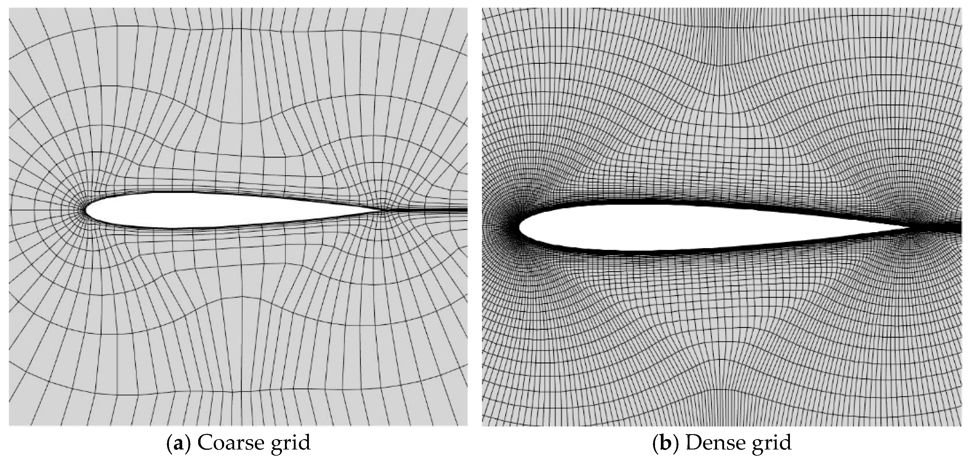
3.1. Low-Speed Flow around an NACA0012 Airfoil

The NACA0012 airfoil, with a symmetric profile and 12% thickness, is considered under the computational condition of $M_{\infty }=0.15$, $\alpha ={5.0}^{\circ }$, $T_{\infty }=288.15K$, ${\mathrm{Re}}_{\infty }=6\times {10}^6$. Two sets of grids with different densities, shown in Figure 2, are utilized for the generation of high- and low-fidelity samples. The number of cells is 3584 and 57,344, respectively. The coarse grid has a grid size that is one-sixteenth of the dense grid, and typically requires fewer iteration steps to reach convergence. However, for the purpose of uniformly assessing computational cost, it is assumed that the low-fidelity samples incur one-sixteenth of the computational cost of the high-fidelity samples.

The wall friction coefficient distribution obtained using standard parameters of the SA model is presented in Figure 3. The high- and low-fidelity results exhibit similar trends, characterized by local abrupt variations on the upper and lower surfaces of the airfoil leading edge, followed by a gradual stabilization. However, significant differences in magnitude are observed, particularly on the upper surface where the dense grid prediction is notably higher. Accurately capturing these local abrupt variations in friction coefficients poses a significant challenge and demands high accuracy from the prediction model.

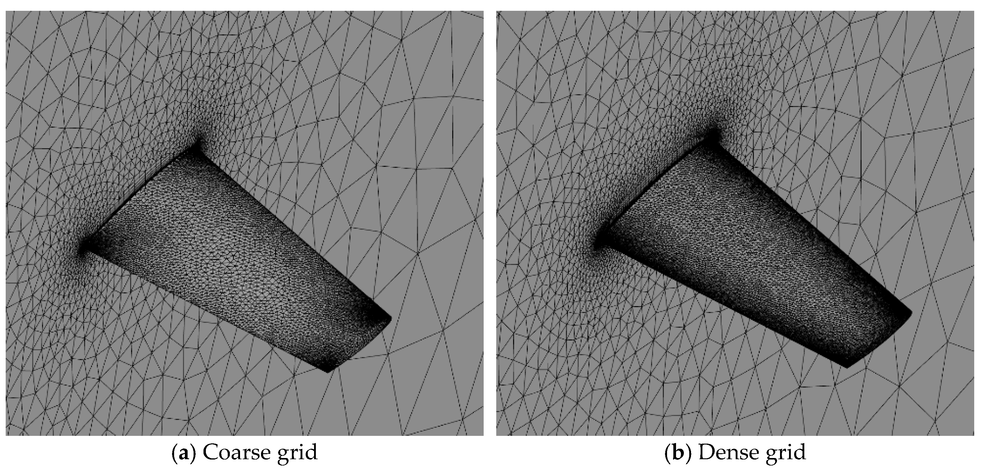
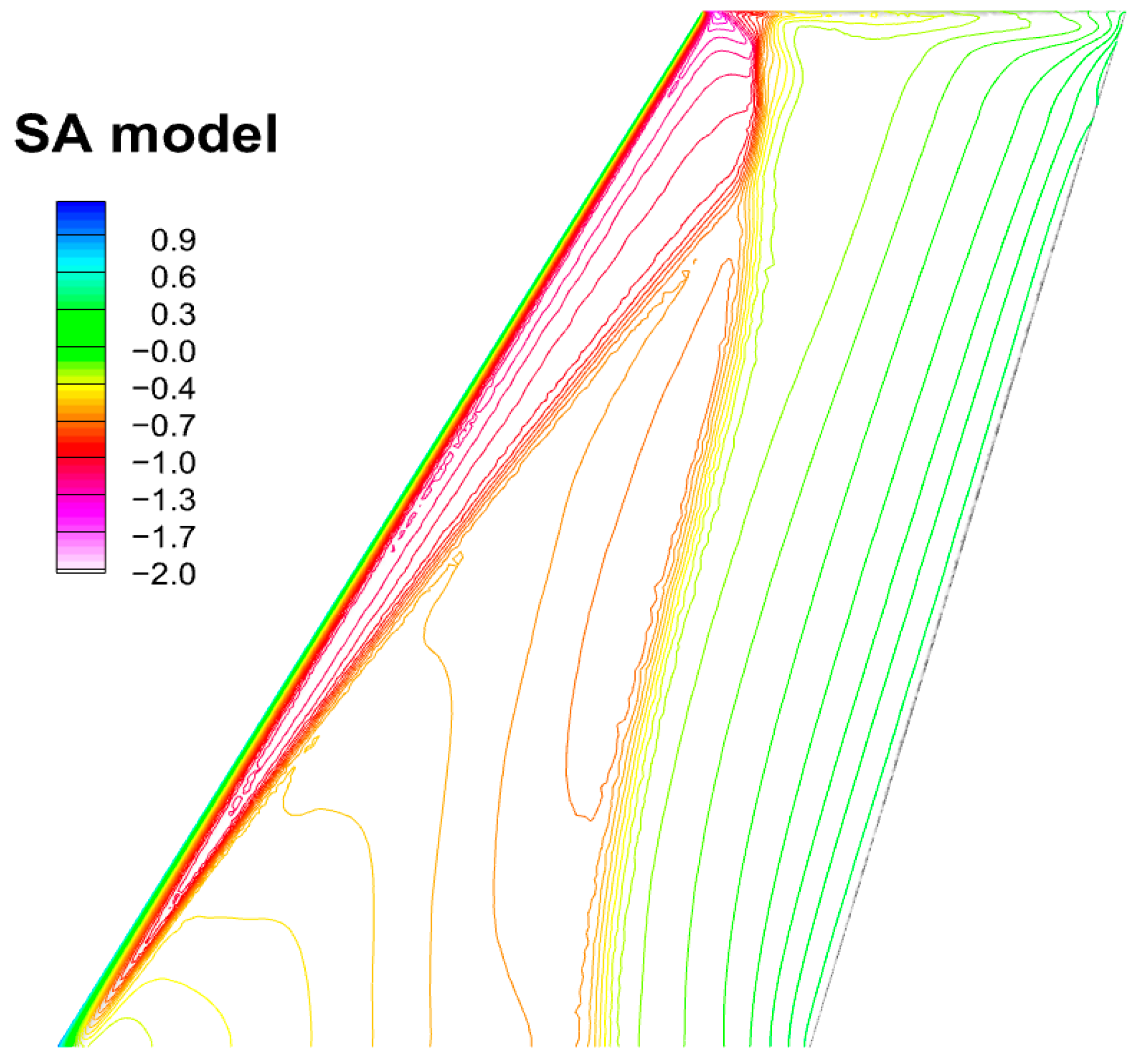
3.2. Transonic Flow around an M6 Wing

The transonic flow over the M6 wing serves as a benchmark test case for assessing transonic flow solvers. The wing features a root chord of approximately 0.8 m and a half-span of approximately 1.2 m, with a symmetric airfoil section. Two sets of grids with different densities, shown in Figure 4, are utilized for the generation of low- and high-fidelity samples. The number of cells is 990,360 and 3,594,863, respectively. Therefore, it is assumed that the acquisition cost of one high-fidelity sample is 3.5 times that of one low-fidelity sample. The output of this case constitutes a vector comprising the pressure coefficients of all grid points covering the entire wing surface, with a dimensionality of 13,638 for the coarse grid and 29,684 for the dense grid.

The computational condition is set at $M_{\infty }=0.8395$, $\alpha ={3.06}^{\circ }$, $T_{\infty }=255.56K$, ${\mathrm{Re}}_{\infty }=1.172\times {10}^7$. Under this condition, a $\lambda$-shaped shock structure develops on the upper surface of the wing, as shown in Figure 5, posing substantial challenges for the prediction model. The pressure distributions obtained by using two sets of grids are consistent, but near the suction peak and shock wave on the upper surface, the dense grid results are in better agreement with the reference experiment results shown in Figure 6.

The sample data in this study are generated using the in-house unstructured grid solver Flowstar [23], which is founded on a cell-centered finite volume methodology and is adept at handling diverse element types, including hexahedra, tetrahedra, prisms, pyramids, and other polyhedra generated via geometrical multigrid techniques. Second-order accuracy in space is attained through linear reconstruction within cells. The vertex-based Green–Gauss approach [24] is employed for gradient computations to uphold accuracy and robustness. To mitigate oscillations in regions of high gradients, Venkatakrishnan’s limiter [25] is utilized. The Roe scheme is engaged for inviscid flux computations. A first-order backward Euler time-differencing scheme with local time stepping is implemented to approximate a steady state, facilitating convergence. The flux Jacobian is derived from a first-order upwind scheme, with the divided convective flux Jacobian composed of the convective flux Jacobian and its spectral radius. The viscous flux Jacobian is approximated using its spectral radius.

In Kriging modeling, the regression function is a constant function, and the covariance function, which determines the spatial correlation structure, is a Gaussian function. In the POD method, the generalized energy criterion is set at 99.9%.

4. Results and Discussion

The prediction accuracy of the model can be assessed through the prediction error of the high-fidelity output vector $s^H$. For incomplete samples within the training dataset, the error vector is defined as $\overrightarrow{\epsilon }={\left.s^H\right|}_{\mathrm{Gappy}\hspace{0.33em}\mathrm{POD}}-{\left.s^H\right|}_{\mathrm{CFD}}$, serving as a metric for evaluating the accuracy of the Gappy POD method. For the testing sample, the error vector is defined as $\overrightarrow{\epsilon }={\left.s^H\right|}_{\mathrm{model}}-{\left.s^H\right|}_{\mathrm{CFD}}$, serving to evaluate the accuracy of the overall model.

For each sample, we define dimensionless errors based on the 1-norm, 2-norm, and infinity norm of the error vector:

$${\epsilon }_1=\frac{{‖\overrightarrow{\epsilon }‖}_1}{n_H\cdot \mathrm{ref}},{\epsilon }_2=\frac{{‖\overrightarrow{\epsilon }‖}_2}{\sqrt{n_H}\cdot \mathrm{ref}},{\epsilon }_{\inf }=\frac{{‖\overrightarrow{\epsilon }‖}_{\inf }}{\mathrm{ref}}$$

where ref is the range of the sample response, $\mathrm{ref}=\max ({\left.s^H\right|}_{\mathrm{CFD}})-\min ({\left.s^H\right|}_{\mathrm{CFD}})$.

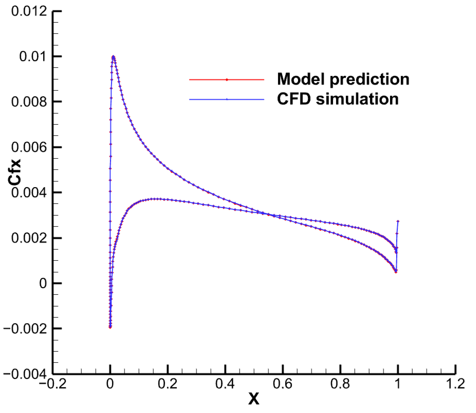
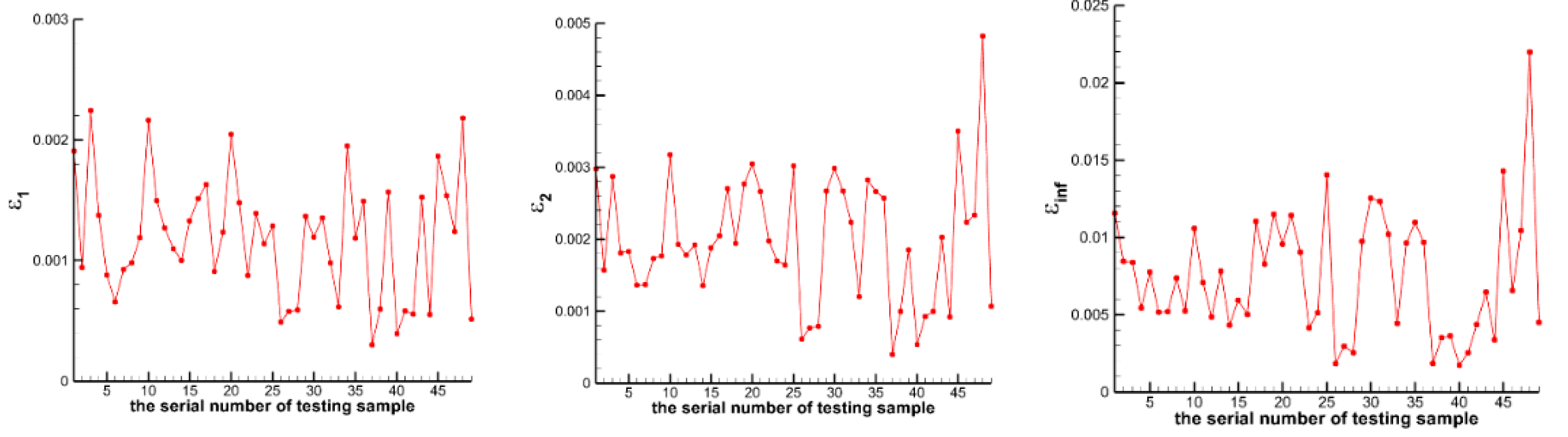
4.1. Low-Speed Flow around an NACA0012 Airfoil

In this case, we fix n_train = 32 and n_test = 49 and assign M values of 11, 13, 15, and 17. This configuration facilitates the analysis of the cost and accuracy trade-offs of the overall model in this paper relative to modeling with high-fidelity samples only. Specifically, the computational cost of 32 low-fidelity samples is deemed equivalent to that of 2 high-fidelity samples.

(1) Accuracy analysis of Gappy POD method

Given that high-fidelity sample data serve as the basis for subsequent POD and Kriging modeling, it is crucial to first analyze the accuracy of the Gappy POD method in reconstructing the corresponding high-fidelity output from low-fidelity output. In the analysis, M is set to 11, with similar results observed for M values of 13, 15, and 17.

Randomly selecting an incomplete sample from the training dataset, Figure 7 presents a comparison between the wall friction coefficient distribution predicted using the Gappy POD method and high-fidelity CFD computation. Visually, the disparity between the two is minimal.

To further evaluate the accuracy of the Gappy POD method, the prediction error was computed for all incomplete samples; the resulting error distribution is depicted in Figure 8. Across all incomplete samples, it can be noted that ε₁ remains below 0.25%, ε₂ remains below 0.6%, and ε_inf remains below 2.5%. Considering the randomness of the Latin hypercube sampling and exchange algorithm, steps (a) through (d) in the training process were repeated a total of 10 times. Figure 9 presents the statistical analysis of errors for all incomplete samples, revealing median values of 0.0007, 0.0015, and 0.0070 for ε₁, ε₂, and ε_inf, respectively. The results demonstrate that the Gappy POD approach is capable of reconstructing high-fidelity outputs using a limited amount of complete sample data and low-fidelity outputs, effectively substituting for computationally expensive high-fidelity CFD calculations and significantly reducing computational costs.

(2) Accuracy analysis of overall model

Given that this study employs the Monte Carlo method to perform extensive random sampling on the overall model, it is imperative to validate the predictive capability of the model. Figure 10 presents a comparison between the wall friction coefficient distribution predicted by the overall model and the high-fidelity CFD computation for a randomly selected sample from the test dataset with M = 11. Visually, the two exhibit excellent agreement.

The prediction error was computed for all testing samples, and the resulting error distribution is depicted in Figure 11. Across all testing samples, it can be noted that ε₁ remains below 0.25%, ε₂ remains below 0.5%, and ε_inf remains below 2.5%. The results strongly validate the predictive capability of the proposed model in accurately estimating the wall friction coefficient distribution for new samples, thus providing robust support for large-scale random sampling processes.

(3) Analysis of the influence of sample size

In the context of multidimensional correlated responses, while the multi-fidelity modeling approach presented in this study is applicable, an alternative approach could involve utilizing solely high-fidelity data for POD decomposition and surrogate model construction. Given that low-fidelity samples, despite their lower acquisition costs, still require CFD computations, a rigorous examination is warranted to determine the precise impact of incorporating additional low-fidelity calculations on the overall modeling accuracy.

To this end, we analyzed the prediction error performance of the model using both the overall model developed in this paper and the approach of using only high-fidelity data for modeling. The results are shown in Figure 12, Figure 13 and Figure 14. To eliminate the randomness of the sampling algorithm, all processes were repeated 10 times. The settings for the POD and the Kriging model were consistent in the comparison. The vertical axis in the three graphs represents the statistical error, while the horizontal axis indicates the models and sample size. Specifically, “11High” represents a single-fidelity model using 11 high-fidelity samples, and “11High32Low” represents a multi-fidelity model using 11 high-fidelity samples and 32 low-fidelity samples. The vertical green solid line divides the horizontal space into several regions, with computational costs in the same region roughly considered equivalent. The figures reveal that as the number of high-fidelity samples used in the multi-fidelity modeling increases from 11 to 17, the overall prediction error remains relatively stable and low, indicating the robustness of the multi-fidelity model. For the model using 11 high-fidelity samples and 32 low-fidelity samples, the median values for ε₁, ε₂, and ε_inf are 0.0012, 0.0018, and 0.0065, respectively, all maintaining a very low error level. For the single-fidelity model, the error decreases significantly as the sample size increases, and it still shows a downward trend even when using 17 high-fidelity samples, indicating that it has not yet stabilized. Furthermore, even when the computational cost is higher than that of the multi-fidelity modeling, the prediction error remains larger. The statistical results fully demonstrate the efficiency and accuracy advantages of the multi-fidelity modeling approach.

(4) Statistical results analysis

Latin hypercube sampling was employed again within the nine-dimensional input space to generate 10⁶ samples, which were sequentially passed to the overall model to derive the corresponding distribution of wall friction coefficients. The statistical analysis of the sample data yielded the mean value and 99% confidence interval of the wall friction coefficient, as depicted in Figure 15. The results indicate significant uncertainty in the friction coefficient across the entire airfoil.

The relative significance of the nine model parameters on the distribution of the friction coefficients can be ascertained through the sensitivity analysis approach, as presented in

Table 2. Sobol indicators of SA model parameters.

	Main Effect	Total Effect
cb1	0.0061	0.0073
σ	0.1223	0.1270
cb2	0.0001	0.0004
κ	0.7945	0.7991
cw2	0.0482	0.0504
cw3	0.0001	0.0001
cv1	0.0200	0.0210
ct3	0.0001	0.0008
ct4	0.0001	0.0004

. A global sensitivity analysis approach proposed by Gamboa et al., which decomposes the covariance of multi-output variables [26], is utilized. As shown, κ emerges as the most influential parameter, which can be expected from a physical standpoint. In the constant Reynolds stress layer of plane shear turbulence, the eddy viscosity coefficient is directly proportional to κ, i.e., ν_t = κu_τd. The eddy viscosity coefficient characterizes the relationship between Reynolds stress and mean flow, serving a role analogous to molecular viscosity in RANS simulations. Hence, κ is intimately linked with the viscosity of the flow, and the friction coefficient is directly correlated with the flow viscosity.

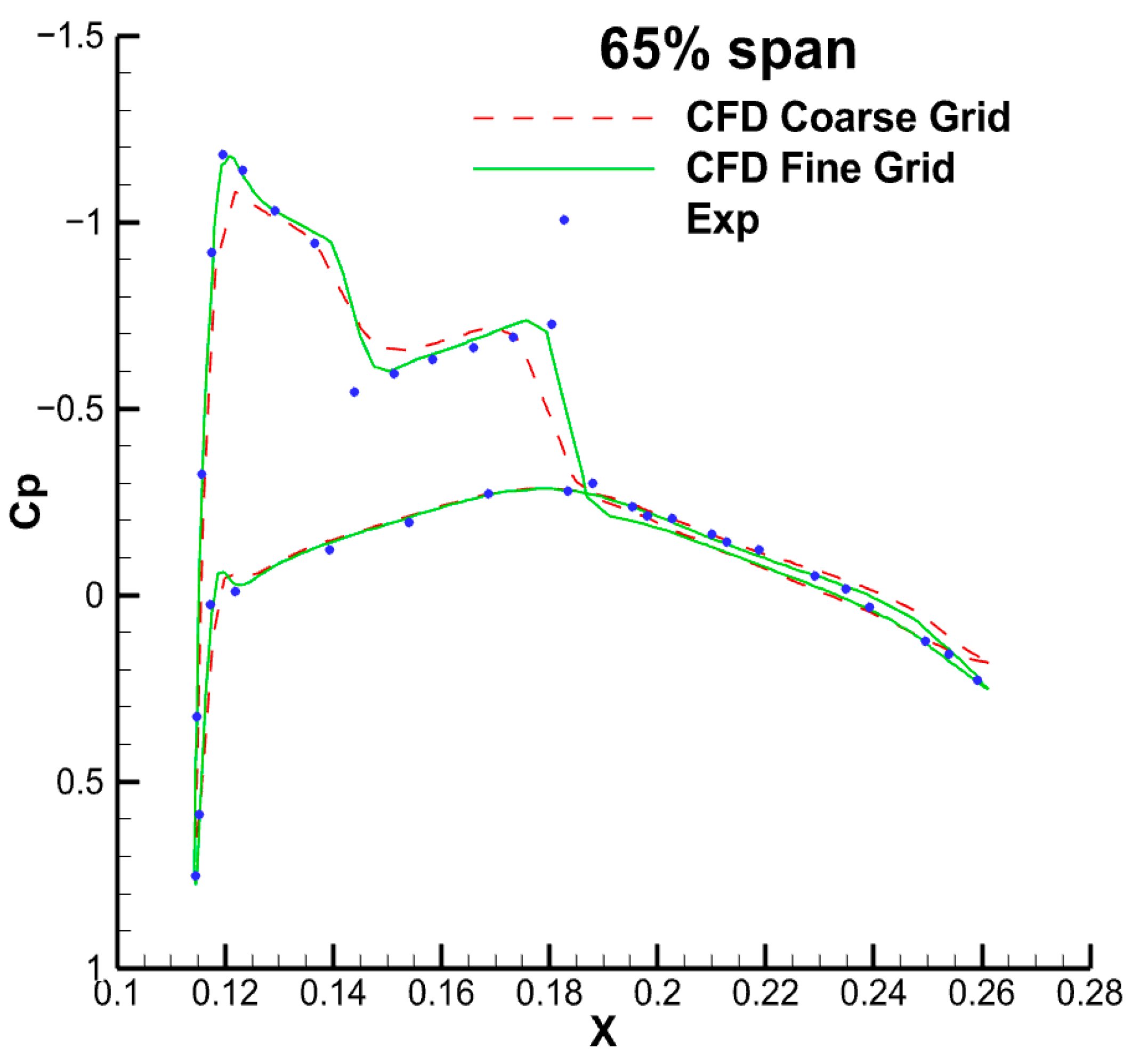
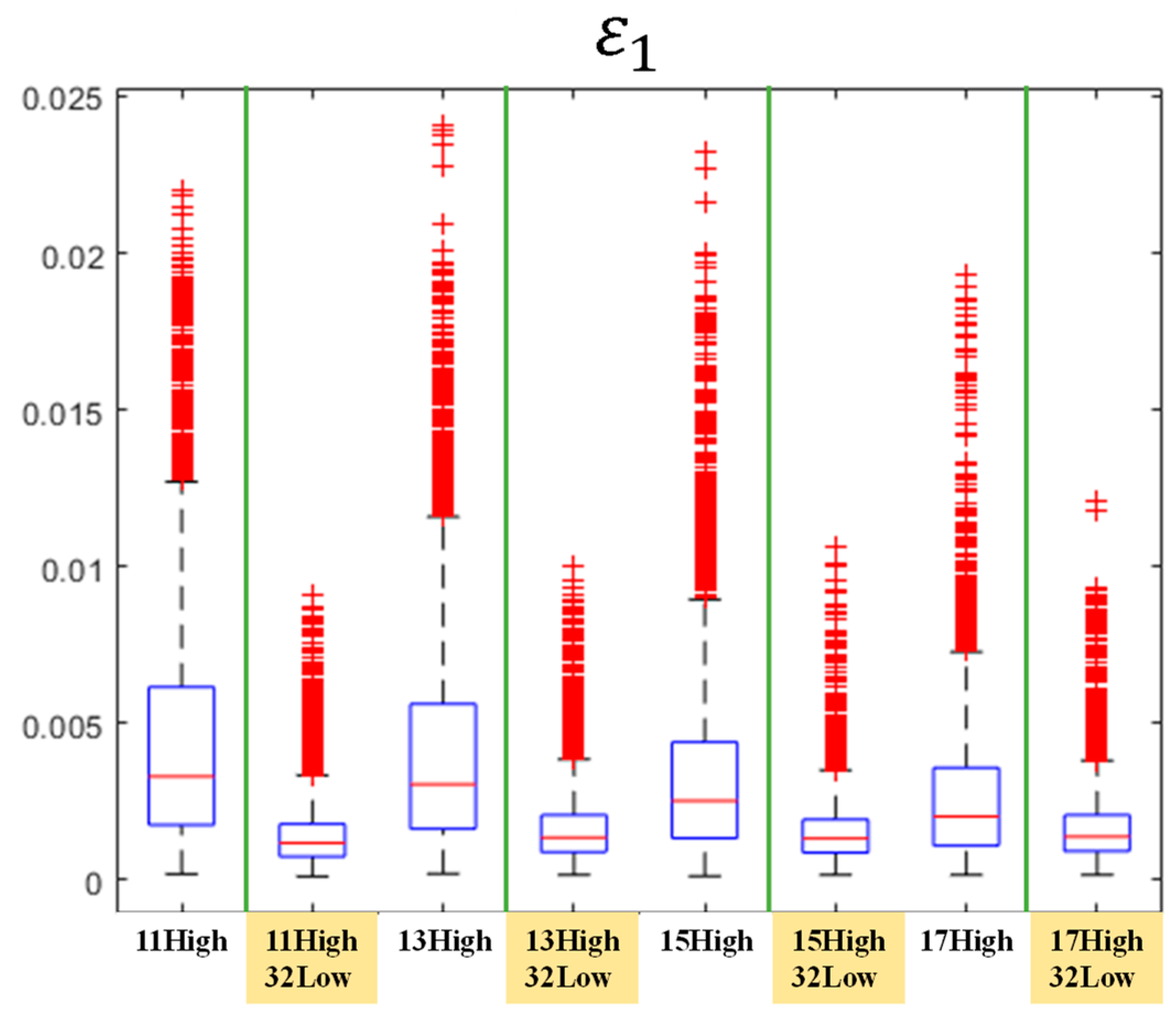
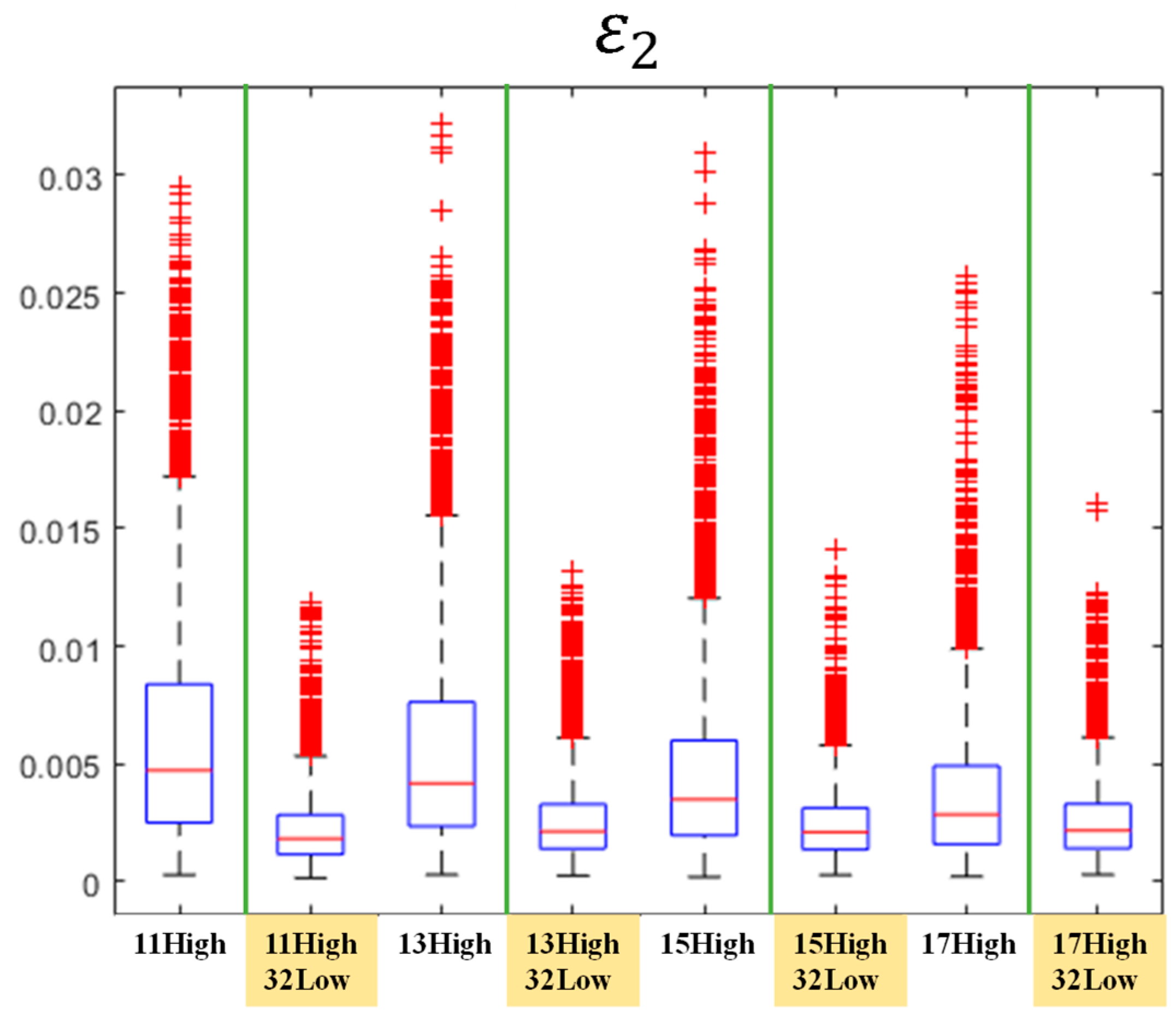
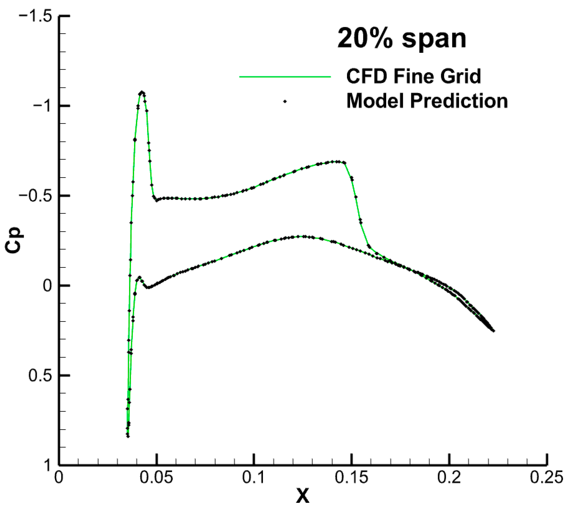
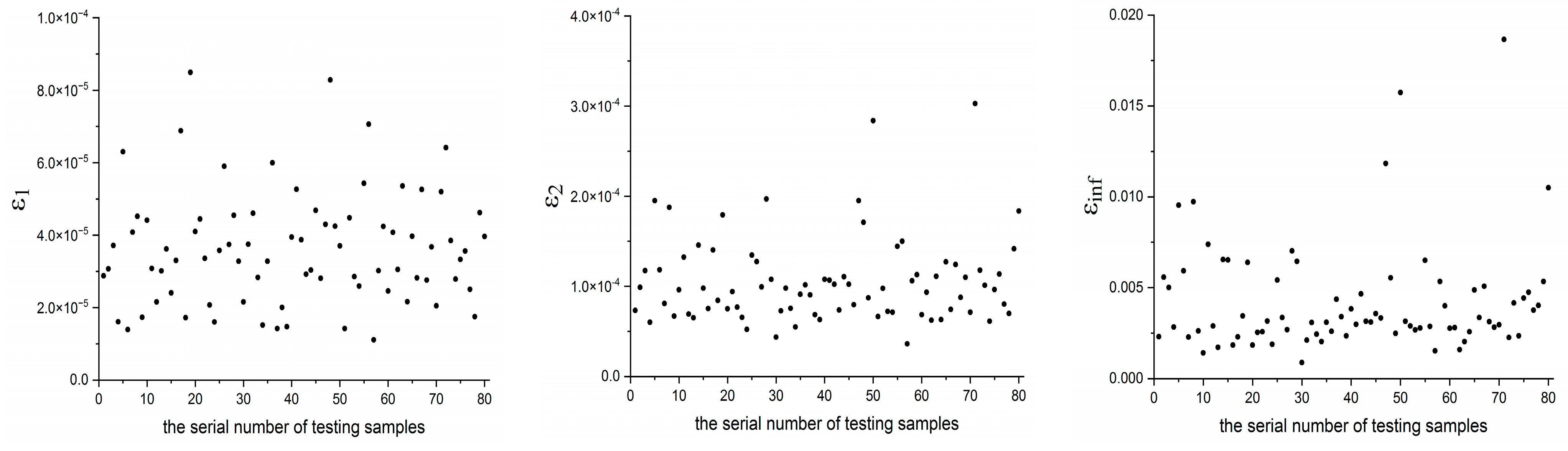
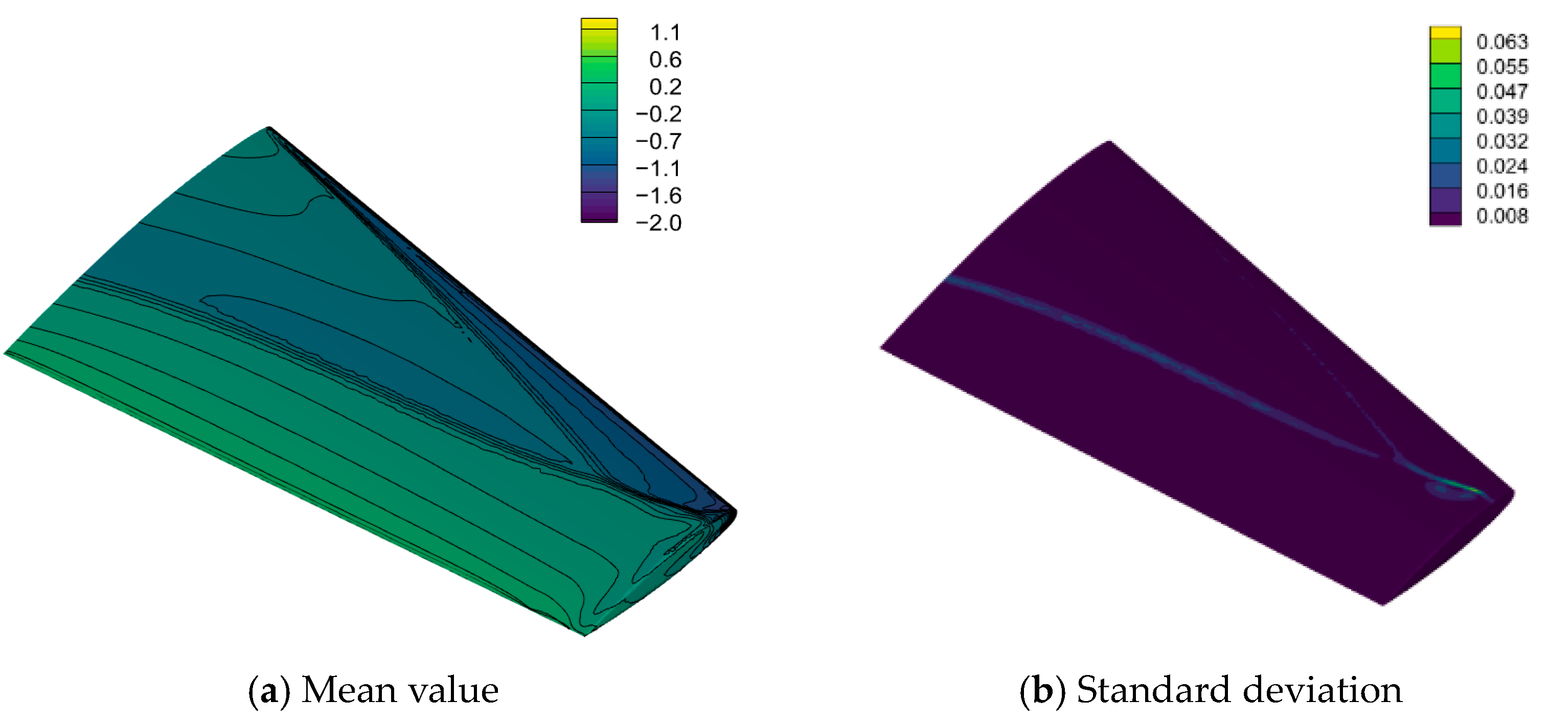
4.2. Transonic Flow around an M6 Wing

(1) Accuracy analysis of Gappy POD method

In the analysis, n_train is set to 21 and M is 6. Randomly selecting an incomplete sample from the training dataset, Figure 16 presents a comparison between the pressure coefficient distribution predicted by the Gappy POD method and the high-fidelity CFD computation. Visually, the disparity between the two is minimal.

To further evaluate the accuracy of the Gappy POD method, the prediction error was computed for all incomplete samples, and the resulting error distribution is depicted in Figure 17. Across all incomplete samples, it can be noted that ${\epsilon }_1$ remains below 0.0035%, ${\epsilon }_2$ remains below 0.03%, and ${\epsilon }_{\inf }$ remains below 1.5%. The results demonstrate that the Gappy POD approach is capable of reconstructing high-fidelity outputs using a limited amount of complete sample data and low-fidelity outputs, effectively substituting for computationally expensive high-fidelity CFD calculations and significantly reducing computational costs.

(2) Accuracy analysis of overall model

The overall model was constructed using n_train high-fidelity responses, of which M responses were calculated using CFD simulations, and the rest were reconstructed using the Gappy POD algorithm from its low-fidelity responses. Figure 18 presents a comparison between the pressure coefficient predicted by the overall model and the high-fidelity CFD computation for a randomly selected sample from the test dataset. Visually, the two exhibit excellent agreement.

The prediction error was computed for all testing samples, and the resulting error distribution is depicted in Figure 19. Across all testing samples, it can be noted that ${\epsilon }_1$ remains below 0.009%, ${\epsilon }_2$ remains below 0.035%, and ${\epsilon }_{\inf }$ remains below 2%. The results strongly validate the predictive capability of the proposed model in accurately estimating the pressure coefficient distribution for new samples, thus providing robust support for large-scale random sampling processes.

(3) Analysis of the influence of sample size

To demonstrate the advantages of the proposed multi-fidelity model over the single-fidelity model using only high-fidelity samples, we analyzed the prediction performance of the two approaches. The computational cost of the low-fidelity sample is converted into the equivalent cost of the high-fidelity sample, with a ratio of 1 to 3.5. The mean prediction error of the two approaches is shown in Figure 20, demonstrating that with the inclusion of low-fidelity samples, the multi-fidelity model can achieve a much lower prediction error with approximately the same computational cost compared with the single-fidelity model.

(4) Statistical results analysis

Latin hypercube sampling was employed again within the nine-dimensional input space to generate 10⁶ samples. These inputs were sequentially fed into the fast prediction model to acquire the corresponding pressure coefficients. The statistical analysis of the sample data yielded the mean value and standard deviation of the wall pressure coefficient, as depicted in Figure 21. Notably, the uncertainty of the pressure coefficient is concentrated at the $\lambda$-shaped shock on the upper surface, whereas the uncertainty at other locations is minimal. This observation aligns with expectations, given that the prediction of shocks is highly sensitive to turbulence model parameters.

Through the application of the multi-output global sensitivity analysis approach grounded in covariance decomposition, the relative significance of model parameters on the pressure coefficient distribution can be ascertained, as presented in

Table 3. Sobol indicators of SA model parameters for M6 case.

	Main Effect	Total Effect
cb1	0.0625	0.0674
σ	0.2375	0.2550
cb2	0.0050	0.0050
κ	0.6079	0.6184
cw2	0.0338	0.0382
cw3	0.0016	0.0017
cv1	0.0340	0.0368
ct3	0.0035	0.0040
ct4	0.0012	0.0012

. Again, κ emerges as the most influential parameter. Following the same analysis as the first case, κ is closely linked with the viscosity of the flow, which significantly impacts the kinetic energy loss of fluid micro-groups within the boundary layer and the capacity to resist adverse pressure gradients, ultimately influencing the prediction of shock wave positions.

5. Conclusions

This study addresses the requirement for uncertainty quantification in multidimensional correlated responses within flow fields. Building on the previously established modeling framework, which utilizes Proper Orthogonal Decomposition for flow field reduction and surrogate models, we introduce a multi-fidelity modeling framework that integrates high- and low-fidelity sample data. The findings of this investigation demonstrate the following:

(1)

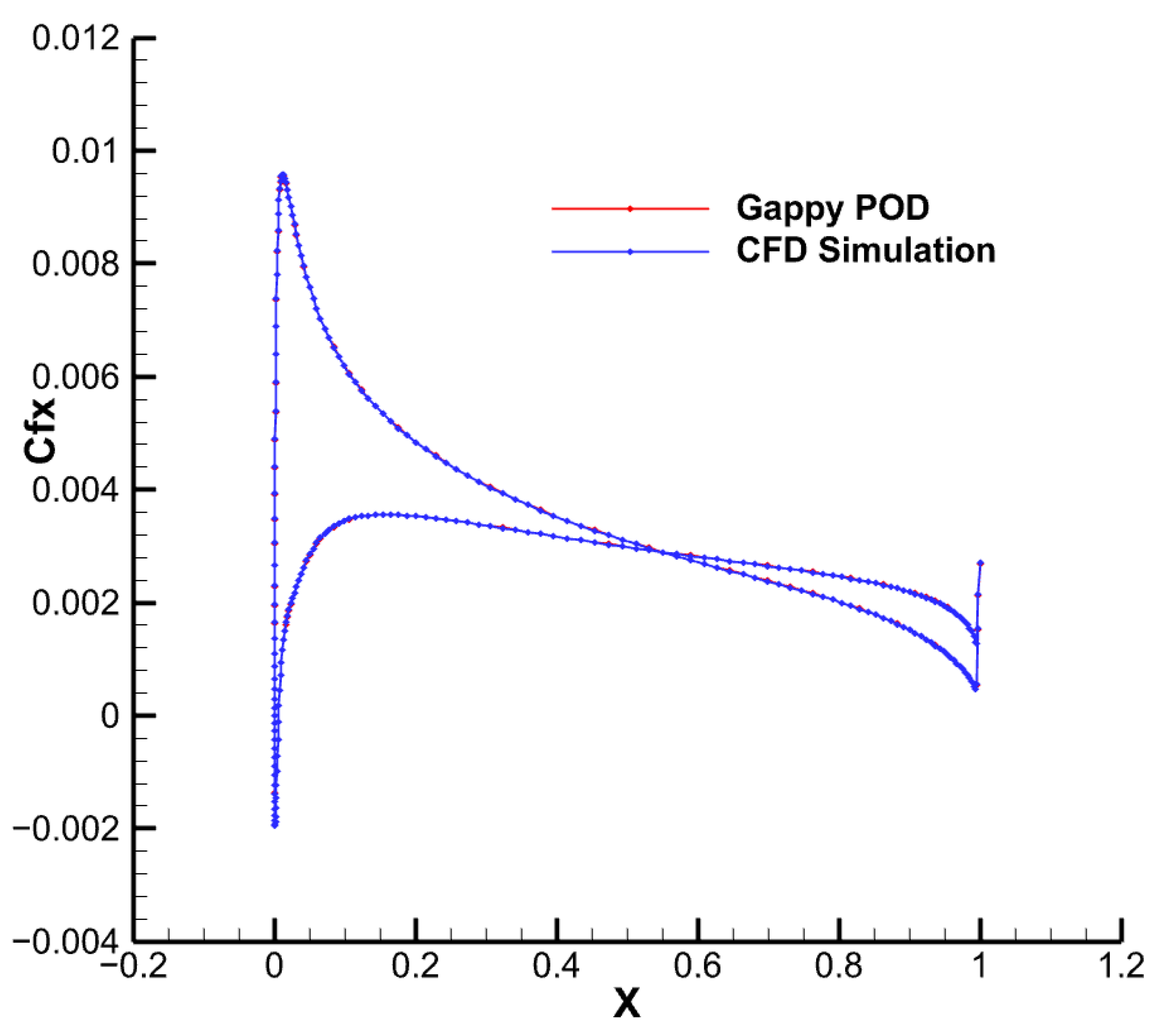
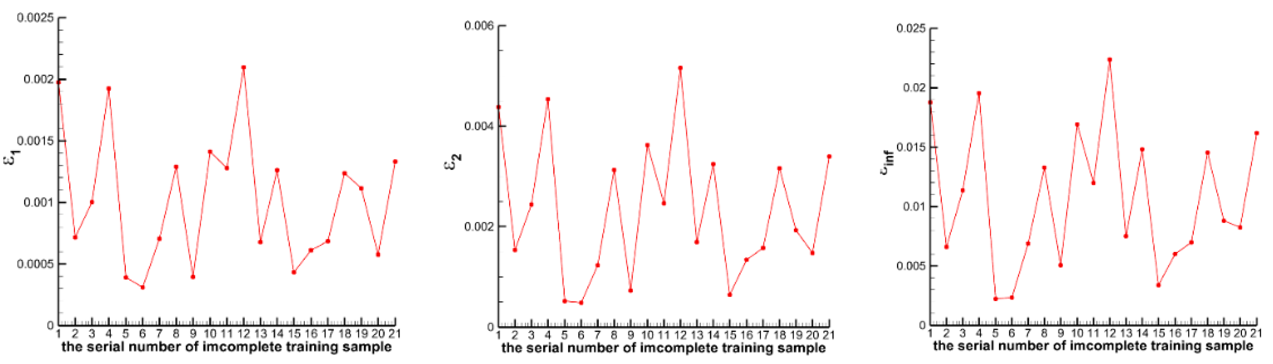
The Gappy POD-based method for supplementing missing data in flow fields enables the restoration of high-fidelity outputs from a limited amount of complete sample data, utilizing the low-fidelity outputs of incomplete samples. This approach effectively avoids the need for computationally expensive high-fidelity CFD calculations on a large number of samples, significantly reducing computational costs.

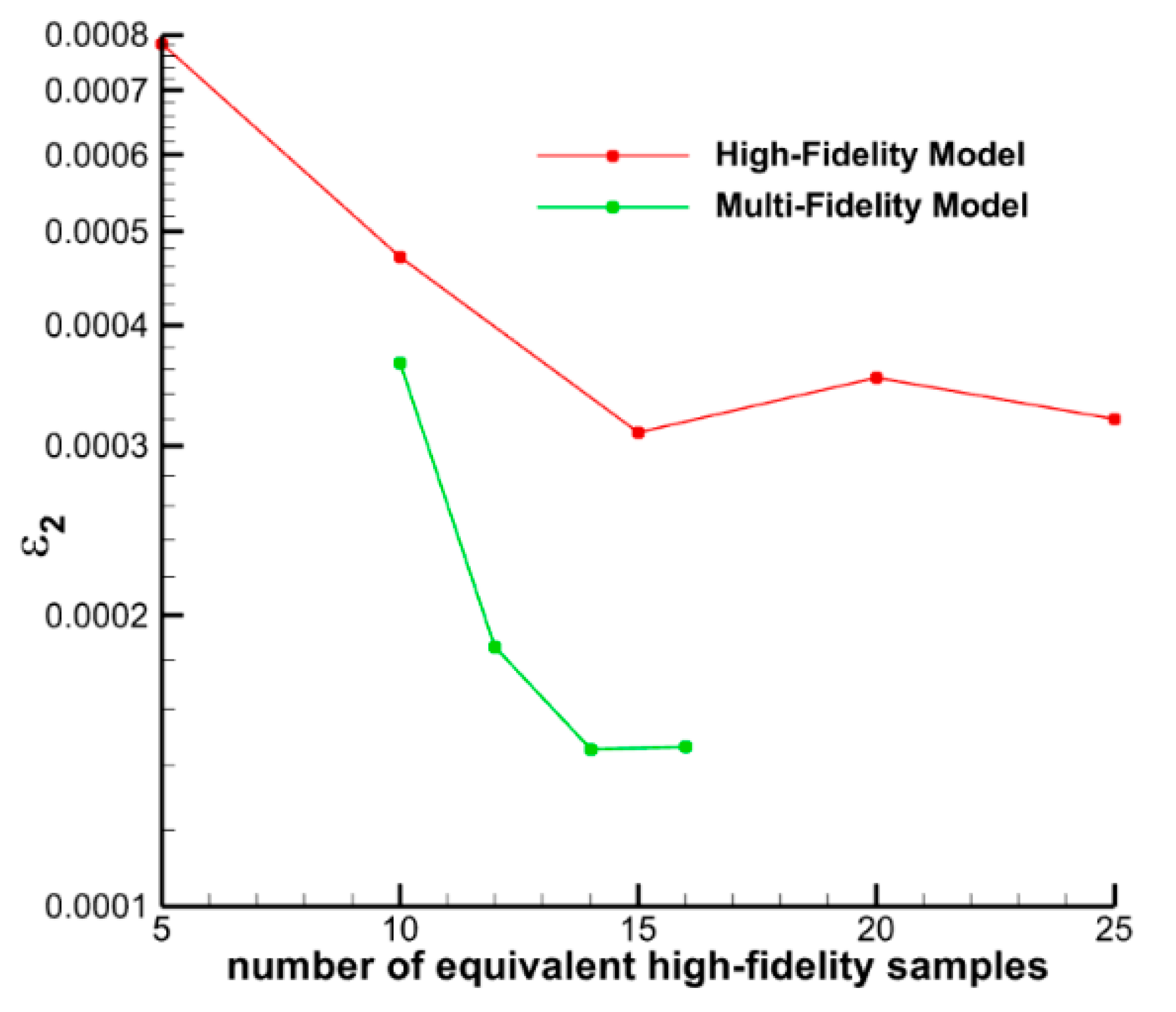
(2)

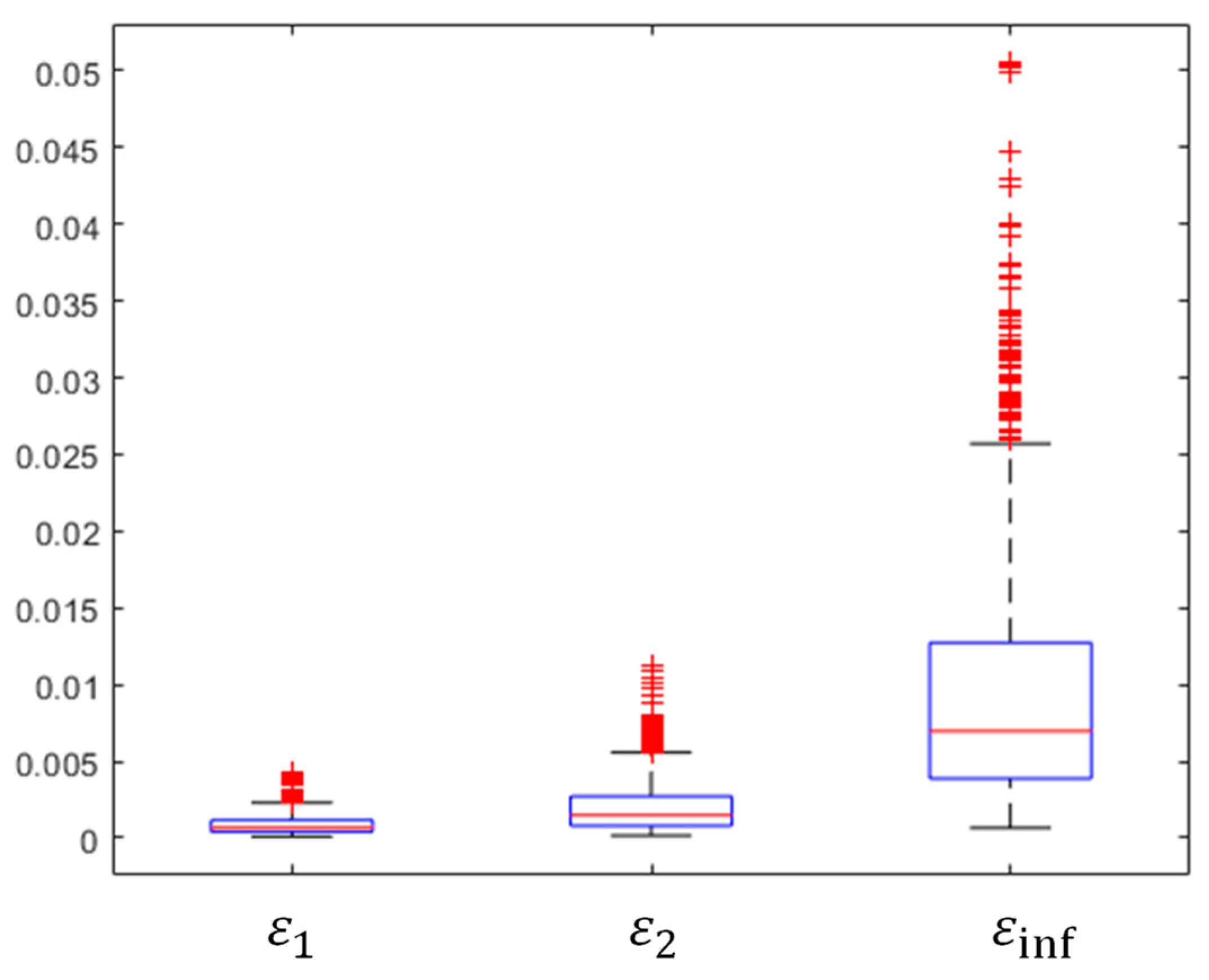
The multi-fidelity modeling approach demonstrates a marked improvement in prediction accuracy and model stability compared to single-fidelity methods while incurring approximately the same computational cost for sample processing. This methodology offers an efficient and robust prediction model for large-scale random sampling.

The cases investigated in this study demonstrate a relatively stable variation in the flow field under differing turbulence model coefficients. In such cases, it is commonly accepted that Proper Orthogonal Decomposition effectively captures the fundamental modes of the flow field. However, if the flow field exhibits rapid changes in response to model parameters, such as smooth flow fields under certain parameters and discontinuous flow fields under others, further validation is required to ascertain the accuracy of the developed model in predicting flow field variables. Autoencoder and deep neural network approaches represent potential solutions to these challenges and will be the focus of future investigations.

References

1. Mehta, U.B.; Eklund, D.R.; Romero, V.J.; Pearce, J.A.; Keim, N.S. Simulation Credibility, Advances in Verification, Validation, and Uncertainty Quantification; NASA/TP-2016-219422; NASA Ames Research Center: Moffett Field, CA, USA, 2016.
2. Xiu, D.; Karniadakis, G. The Wiener-Askey Polynomial Chaos for Stochastic Differential Equations. SIAM J. Sci. Comput. 2002, 24, 619–644. [Google Scholar] [CrossRef]
3. Li, M.; Wang, Z. Surrogate Model Uncertainty Quantification for Reliability-based Design Optimization. Reliab. Eng. Syst. Saf. 2019, 192, 106432. [Google Scholar] [CrossRef]
4. Bhattacharyya, B. Uncertainty quantification of dynamical systems by a POD–Kriging surrogate model. J. Comput. Sci. 2022, 60, 101602. [Google Scholar] [CrossRef]
5. Li, X.; Zou, Z.-J.; Wang, Z.-H.; Zou, L.; Gao, H. Surrogate model based uncertainty quantification of CFD simulations of the viscous flow around a ship advancing in shallow water. Ocean. Eng. 2021, 234, 109206. [Google Scholar]
6. Tripathy, R.K.; Bilionis, I. Deep UQ: Learning deep neural network surrogate models for high dimensional uncertainty quantification. J. Comput. Phys. 2018, 375, 565–588. [Google Scholar] [CrossRef]
7. Kennedy, M.C.; O’Hagan, A. Predicting the Output from a Complex Computer Code When Fast Approximations Are Available. Biometrika 2000, 87, 1–13. [Google Scholar] [CrossRef]
8. Forrester, A.I.J.; Sóbester, A.; Keane, A.J. Multi-fidelity optimization via surrogate modelling. Proc. R. Soc. A 2007, 463, 3251–3269. [Google Scholar] [CrossRef]
9. Zimmermann, R.; Han, Z.H. Simplified cross-correlation estimation for multifidelity surrogate cokriging models. Adv. Appl. Math. Sci. 2010, 7, 181–202. [Google Scholar]
10. Meng, X.; Karniadakis, G.E. A composite neural network that learns from multi-fidelity data: Application to function approximation and inverse PDE problems. J. Comput. Phys. 2019, 401, 109020. [Google Scholar] [CrossRef]
11. Motamed, M. A multi-fidelity neural network surrogate sampling method for uncertainty quantification. J. Comput. Phys. 2021, 426, 109923. [Google Scholar] [CrossRef]
12. Cook, R.D.; Nachtsheim, C.J. A comparison of algorithms for constructing exact D-optimal designs. Technometrics 1980, 22, 315–324. [Google Scholar] [CrossRef]
13. Morris, M.D.; Mitchell, T.J. Exploratory designs for computer experiments. J. Stat. Plan. Inference 1995, 43, 381–402. [Google Scholar] [CrossRef]
14. Everson, R.; Sirovich, L. Karhunen-Loeve procedure for gappy data. J. Opt. Soc. Am. A 1995, 12, 1657–1664. [Google Scholar] [CrossRef]
15. Benamara, T.; Breitkopf, P.; Lepot, I.; Sainvitu, C. Adaptive infill sampling criterion for multi-fidelity optimization based on Gappy-POD Application to the flight domain study of a transonic airfoil. Struct. Multidiscip. Optim. 2016, 54, 843–855. [Google Scholar] [CrossRef]
16. Lumley, J.L. The Structure of Inhomogeneous Turbulent Flows. Commun. Pure Appl. Math. 1967, 20, 453–488. [Google Scholar] [CrossRef]
17. Sirovich, L.; Kirby, M. Low-dimensional procedure for the characterization of human faces. J. Opt. Soc. Am. A 1987, 4, 519–524. [Google Scholar] [CrossRef] [PubMed]
18. Krige, D.G. A statistical approach to some basic mine valuation problems on the Witwatersrand. J. Chem. Metall. Min. Eng. Soc. S. Afr. 1951, 52, 119–139. [Google Scholar]
19. Sacks, J.; Welch, W.J.; Mitchell, T.J.; Wynn, H.P. Design and analysis of computer experiments. Stat. Sci. 1989, 4, 409–423. [Google Scholar] [CrossRef]
20. Spalart, P.R.; Allmaras, S.R. A One-Equation Turbulence Model for Aerodynamic Flows. AIAA J. 1992, 30, 5–12. [Google Scholar] [CrossRef]
21. Schaefer, J.; Cary, A.; Mani, M.; Spalart, P. Uncertainty Quantification and Sensitivity Analysis of SA Turbulence Model Coefficients in Two and Three Dimensions. In Proceedings of the 55th AIAA Aerospace Sciences Meeting, Grapevine, TX, USA, 9–13 January 2017. AIAA Paper 2017-1710. [Google Scholar]
22. Stephanopoulos, K.; Witte, I.; Wray, T.J.; Agarwal, R.K. Uncertainty Quantification of Turbulence Model Coefficients in OpenFOAM and Fluent for Mildly Separated Flows. In Proceedings of the 46th AIAA Fluid Dynamics Conference, Washington, DC, USA, 13–17 June 2016. AIAA Paper 2016-4401. [Google Scholar]
23. Chen, J.Q.; Wu, X.J.; Zhang, J.; Li, B.; Jia, H.Y.; Zhou, N.C. Flowstar: General Unstructured-grid CFD Software for National Numerical Wind Tunnel (NNW) Project. Acta Aeronaut. Astronaut. Sin. 2021, 42, 625739. (In Chinese) [Google Scholar]
24. Diskin, B.; Thomas, J.L. Comparison of Node-Centered and Cell-Centered Unstructured Finite Volume Discretizations: Inviscid Fluxes. AIAA J. 2011, 49, 836–854. [Google Scholar] [CrossRef]
25. Venkatakrishnan, V. On the Accuracy of Limiters and Convergence to Steady-State Solutions. In Proceedings of the 31st Aerospace Sciences Meeting, Reno, NV, USA, 11–14 January 1993. AIAA Paper 1993-0880. [Google Scholar]
26. Gamboa, F.; Janon, A.; Klein, T.; Lagnoux, A. Sensitivity Analysis for Multidimensional and Functional Outputs. Electron. J. Stat. 2014, 8, 575–603. [Google Scholar] [CrossRef]
Figure 1. Overall flow chart for multi-fidelity uncertainty propagation model.
Aerospace 11 00263 g001
Figure 2. Computational grid for NACA0012 airfoil.
Aerospace 11 00263 g002
Figure 3. Wall friction coefficient distribution for NACA0012 airfoil under standard SA model parameters.
Aerospace 11 00263 g003
Figure 4. Computational grid for M6 wing.
Aerospace 11 00263 g004
Figure 5. Pressure contours for M6 wing under standard model parameters using fine grid.
Aerospace 11 00263 g005
Figure 6. Pressure coefficient distribution for M6 wing under original SA model parameter at 65% wingspan.
Aerospace 11 00263 g006
Figure 7. Comparison between the wall friction coefficients predicted using the Gappy POD method and high-fidelity CFD computation for the NACA0012 case.
Aerospace 11 00263 g007
Figure 8. Error analysis of Gappy POD method for predictions on incomplete samples for the NACA0012 case.
Aerospace 11 00263 g008
Figure 9. Statistical error analysis of Gappy POD method for predictions on incomplete samples (repeated 10 times).
Aerospace 11 00263 g009
Figure 10. Comparison between the wall friction coefficients predicted by the overall model and the high-fidelity CFD computation.
Aerospace 11 00263 g010
Figure 11. Error analysis of overall model for predictions on testing samples for the NAC0012 case.
Aerospace 11 00263 g011
Figure 12. Statistical error analysis for predictions on testing samples (ε1).
Aerospace 11 00263 g012
Figure 13. Statistical error analysis for predictions on testing samples (ε2).
Aerospace 11 00263 g013
Figure 14. Statistical error analysis for predictions on testing samples (εinf).
Aerospace 11 00263 g014
Figure 15. Mean value and 99% confidence interval of the wall friction coefficient.
Aerospace 11 00263 g015
Figure 16. Comparison between the pressure coefficients predicted using the Gappy POD method and the high-fidelity CFD computation for the M6 case.
Aerospace 11 00263 g016
Figure 17. Error analysis of Gappy POD method for predictions on incomplete samples for the M6 case.
Aerospace 11 00263 g017
Figure 18. Comparison between the pressure coefficients predicted by the overall model and the high-fidelity CFD computation for the M6 case.
Aerospace 11 00263 g018
Figure 19. Error analysis of overall model for predictions on testing samples for the M6 case.
Aerospace 11 00263 g019
Figure 20. Comparison of prediction error on testing samples between multi-fidelity and high-fidelity models for the M6 case.
Aerospace 11 00263 g020
Figure 21. Contours of mean value and standard deviation of the wall pressure coefficients.
Aerospace 11 00263 g021