Fuzzy Modeling Framework Using Sector Non-Linearity Techniques for Fixed-Wing Aircrafts

Abstract

This paper presents a mathematical modeling approach utilizing a fuzzy modeling framework for fixed-wing aircraft systems with the goal of creating a highly desirable mathematical representation for model-based control design applications. The starting point is a mathematical model comprising fifteen non-linear ordinary differential equations representing the dynamic and kinematic behavior applicable to a wide range of fixed-wing aircraft systems. Here, the proposed mathematical modeling framework is applied to the AIRBUS A310 model developed by ONERA. The proposed fuzzy modeling framework takes advantage of sector non-linearity red techniques to recast all the non-linear terms from the original model to a set of combined fuzzy rules. The result of this fuzzification is a more suitable mathematical description from the control system design point of view. Therefore, the combination of this fuzzy model and the wide range of control techniques available in the literature for such kind of models, like parallel and non-parallel distributed compensation control laws using linear matrix inequality optimization, enables the development of control algorithms that guarantee stability conditions for a wide range of operations points, avoiding the classical gain scheduling schemes, where the stability issues can be extremely challenging.

1. Introduction

Piloting a modern aircraft, including of crewed, remotely piloted, and fully autonomous types, relies on automatic control systems to insure robust stability and high performance under a wide variety of conditions. Robust stability, often measured by phase and gain margin, is a closed-loop concept that quantifies the ability of a feedback control system to remain stable in the presence of uncertainties, both in the mathematical model and in cases of unexpected changes in the external environmental conditions. The level of performance required is application-specific and often measured in terms of rise time, overshoots, settling time, and other time-domain performances. Many phases of flight, such as final approach with autonomous landing, demand that many variables representing the aircraft attitude state (e.g., aircraft body reference frame relative to a ground reference frame) and translational state (e.g., position and velocity relative to the ground) are controlled simultaneously. The level of complexity of any model-based control system design process coupled with the ability to guarantee robust stability and the requisite closed-loop performance depends on an accurate mathematical aircraft model describing both the translational motion and the orientation. In general, the more closely the mathematical model reflects the specific aircraft and the environment it flies in (that is, the real world), the better the actively controlled closed loop system performance. Improvements in control system design methodologies stemming from the availability of accurate yet tractable mathematical models when combined with effective navigation systems directly contributes to safe, high-performance flight.

The classical mathematical model of the aircraft translation and orientation comprises fifteen non-linear differential equations [1]. Many control system design methodologies employ linearized mathematical models based on Taylor series approximation of the fifteen non-linear differential equations about an equilibrium point representing a flight regime of interest. For example, it is a well known and often studied problem of providing a smooth flight of a passenger aircraft in the presence of wind turbulence. The mathematical model can be linearized using wing level; constant velocity flight condition and the feedback control system design based on linear mathematical models strive to keep the flight smooth and near that equilibrium condition. Large deviations from the equilibrium condition, say, due to an unexpected large wind shear, can move the aircraft out of the linear region and potentially lead to performance and stability issues. In a single flight, there are many flight regimes from take-off to landing represented by different equilibrium points. One of the extended solutions for this issue is the combination of different controllers with the same structure (i.e., gain scheduling) [2].

This paper presents dynamic models for aircraft control design, which implies accurate models with suitable structures for optimizing the control design stage. One of the aims of this paper is to present a general modeling framework based on fuzzy logic for control design rather than linearization around various equilibrium points. This work explores ways to obtain a general fuzzy model of a fixed-wing aircraft using the sector non-linearity technique due to its proven ability to describe dynamic behavior in the field of non-linear systems (page 6 of [3,4,5,6]). The significant advantage of obtaining a fuzzy representation of the original aircraft dynamic model is the possibility to design controllers like parallel (PDC) and non-parallel (non-PDC) distributed compensation control laws [5,7,8] using linear matrix inequality (LMI) optimization [9]. These control algorithms guarantee stability conditions for a wide range of operation points and flight conditions using the same controller, avoiding the classical gain scheduling schemes where stability issues can be highly challenging.

The application of fuzzy logic in the field of aerospace applications has been inherent to the emergence of the first contributions in this area, as shown in [10,11,12]. These earlier works explored the use of fuzzy logic as alternatives in control algorithms, state estimation or fault detection. Afterwards, several contributions have been presented where experimental data and clustering techniques have been combined with fuzzy logic for the identification of dynamic models (black-box type) and/or controllers. Some examples are [13,14,15].

Since the use of fuzzy logic has provided satisfactory results almost from its first applications, it has been widely used in many different areas of the aerospace sector such as dynamic control in hyper-sonic aircraft surfaces [16], health monitoring for aircraft engines [17], autopilots for helicopters [18] or soft sensors for angle-of-attack (AoA) estimation [19,20]. Furthermore, the application of fuzzy logic in novel areas of the aerospace sector, such as Unmanned Aerial Vehicles (UAVs) or Autonomous Underwater Vehicles (AUVs), is also currently an area of interest, as shown in [21,22,23,24,25,26].

The approach presented in this work is to define a global non-linear fuzzy model representing the global aircraft dynamics. In general, there are two approaches for constructing fuzzy models: (i) identification using input–output data (as mentioned before [13,14,15,27]), and (ii) derivation from given non-linear system equations. The proposed fuzzy modeling framework is focused on the second approach and uses the idea of sector non-linearity. This method was introduced by Tanaka and Wang in (page 10 of [3]), and it enables the formulation of an equivalent fuzzy model from an original non-linear system using linear subsystems. This approach has been addressed previously in the aerospace field, as shown, for example, in [26,28,29].

The sector non-linearity technique is based on representing any static non-linear term $k\left(t\right)$ of a model with a fuzzy quantity, where the jth rule is of the form

IF $z_{n_1}\left(t\right)$ is $M_{z_{n_1}}^{i_{n_1}}$ and … and $z_{n_s}\left(t\right)$ is $M_{z_{n_s}}^{i_{n_s}}$

$$\begin{array}{c}\mathbf{THEN}\begin{array}{cc}k\left(t\right)=A_k^j\left(t\right)\hfill & \hfill j=1,\dots ,2^s\end{array}\\ j=i_{n_1}+i_{n_2}·2^1+\dots +i_{n_s}·2^{s-1},i_{n_h}\in \{1,2\}\\ h=1,\dots ,s,\end{array}$$

(1)

where $z_{n_h}\left(t\right)$ are the premise variables, $M_{z_{n_h}}^{i_{n_h}}$ are the membership functions and $A_k^j\left(t\right)$ are constant values (zero-order model) or linear functions depending on state variables $x\left(t\right)$ (first-order model) of non-linear models. The premise variables are known functions which may depend on the state variables and/or time [30].

In this paper, the main objective is to present a new version of the conventional fixed-wing aircraft dynamic model that uses fuzzy logic methods, in particular a way to obtain an equivalent and complete fuzzy model of such non-linear model. This is the main contribution of this work, which distinguishes it from other contributions such as [28,29], where the dynamics of the aircraft are only partially described (longitudinal model), the rotation matrices between the different axes are not included and simplifications are performed through the application of Taylor series to make the problem more solvable. For all these reasons, this article proposes a much more general framework that allows to obtain a global and complete model with a higher accuracy.

Finally, in future research, a Takagi–Sugeno fuzzy model (page 6 of [3]) will be developed starting from the fuzzy model obtained in this manuscript. This Takagi–Sugeno model will be used to design non-linear TS fuzzy controllers. On the one hand, for a better understanding, the validation and examples of the proposed fuzzy modeling are performed using parameters of an Airbus A310 aircraft [31].

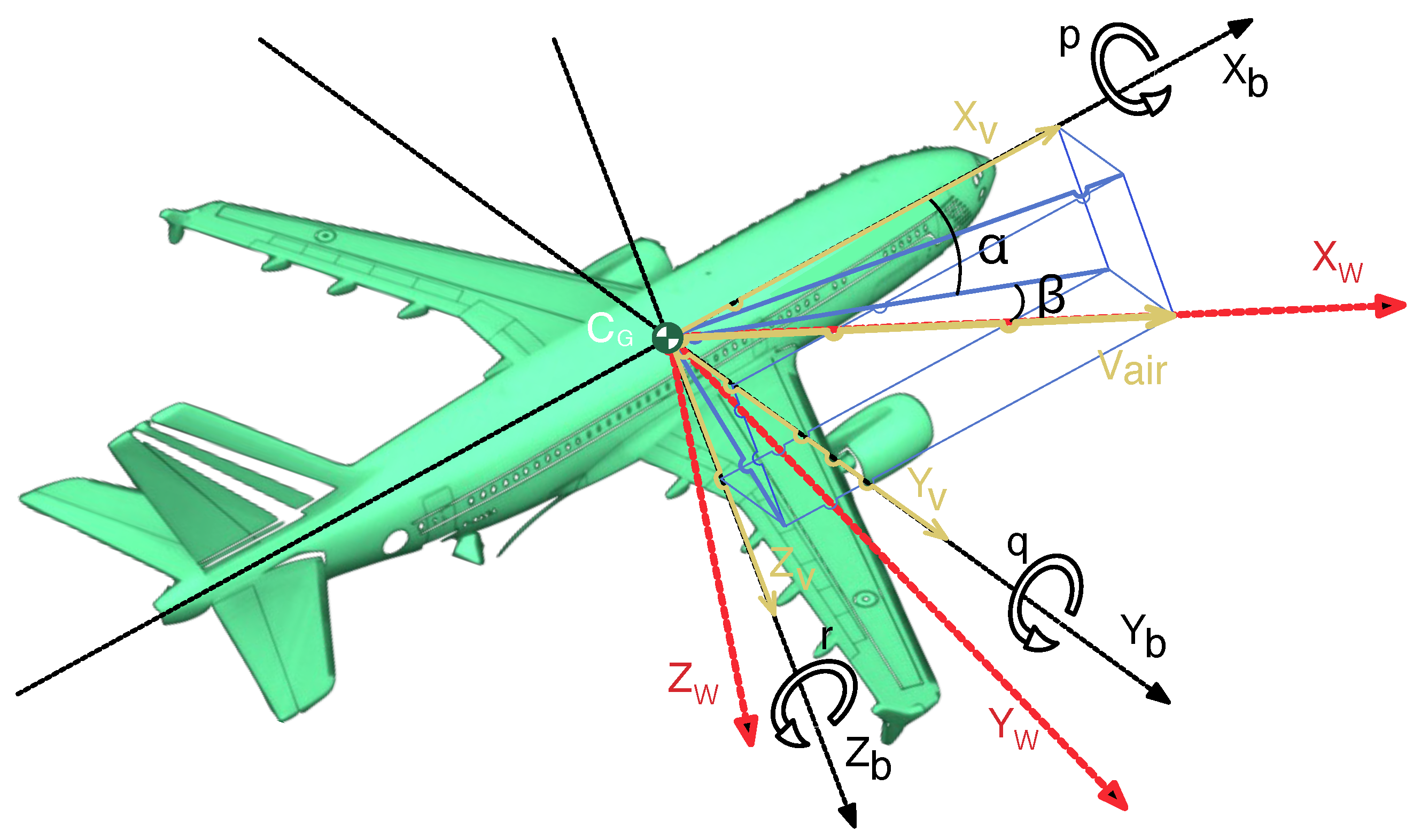
This paper is organized as follows. In Section 2, the classical aircraft dynamic model is presented, where the attitude dynamics are represented by quaternions. Section 3 introduces the sector non-linearity technique for fuzzy modeling. Section 4 provides the construction of the fuzzy model by selecting model limits and applying them in the dynamic model. Section 5 presents simulation results and validation with the Onera non-linear model benchmark of A310 [31]. Section 6 offers conclusions.

2. Classic Aircraft Model with Quaternions

2.1. Quaternions in Aircraft Dynamic Models

It is common to use Euler angles to represent aircraft orientation. They have a very physical interpretation, more readily enabling visualization of orientation by humans. However, when utilizing Euler angles, it is possible to experience the so-called gimbal lock. For example, if using a roll–pitch–yaw description of the orientation, gimbal lock is a numerical condition that occurs when the pitch angle is ±90°. A potential solution, therefore, is to represent the orientation in some other way. Quaternions are widely used as attitude representation parameters for rigid bodies such as aircrafts [32,33]. For the dynamic aircraft models in this paper, quaternions are used to represent the orientation between the various reference frames due to their computational efficiency and excellent numerical properties. Computing Euler angles and associated coordinate transformation matrices to and from quaternions is readily accomplished. The three main reference frames utilized here are the body axis reference frame, the Earth-linked reference frame, and the wind axis reference frame described below. Quaternions are used to represent the orientation of the various Earth-linked vertical reference frames to the aircraft body axis reference frames, as well as the orientation between the aircraft wind axes reference frame and the aircraft body axes reference frame (Figure 1).

• Body axis reference frame $[x_b,y_b,z_b]$: is the origin at the center of gravity fixed to the aircraft structure. The x-axis is the longitudinal aircraft axis in which the positioning direction is forward, the y-axis is perpendicular to the aircraft plane of symmetry-positive direction out the right wing, and the z-axis is perpendicular to the other two and oriented downward.
• Earth-linked axis reference frame $[x_v,y_v,z_v]$: moves with the aircraft and its origin; it is also the center of gravity. The x-axis is oriented to the North, the y-axis to the East and z-axis perpendicular to the other two and oriented downward. The x-y plane is parallel to the Earth’s surface.
• Wind axis reference frame $[x_w,y_w,z_w]$: is a particular body axis frame because the x-axis is aligned with the airspeed velocity vector which is always tangent to the trajectory. The y-axis is perpendicular to the x-axis in the same plane as $x_b$ and $y_b$, and the z-axis is perpendicular to the other two and oriented downward.

To increase the numerical robustness of the aircraft attitude, that is to say, to avoid the so-called gimbal lock, a set of parameters is formulated using the same reference frame in each equation of the aircraft dynamic model. For that reason, it is important to define the quaternion transformation coordinate matrix. The transformation matrix from body axis reference frame to the Earth-linked frame [32,33] is represented by 

$$\begin{array}{c}{R}_{b\to v}\left(Q\left(t\right)\right)=\\ \left(\begin{array}{ccc}{q}_0^2+q_1^2-q_2^2-q_3^2& 2(q_1{q}_2-q_3{q}_0)& 2(q_1{q}_3+q_2{q}_0)\\ 2(q_1{q}_2+q_3{q}_0)& q_0^2-q_1^2+q_2^2-q_3^2& 2(q_2{q}_3-q_1{q}_0)\\ 2(q_1{q}_3-q_2{q}_0)& 2(q_2{q}_3+q_1{q}_0)& q_0^2-q_1^2-q_2^2+q_3^2\end{array}\right)\end{array}$$

(2)

where $Q\left(t\right)={[q_0,q_1,q_2,q_3]}^T$ is the attitude quaternion that satisfies $\left|\right|Q\left(t\right)\left|\right|=1$ for all t. Matrix $R_{b\to v}\left(Q\left(t\right)\right)$ is an orthonormal matrix, hence $R_{v\to b}\left(Q\left(t\right)\right)=R_{b\to v}{\left(Q\left(t\right)\right)}^T$. To visualize the aircraft attitude, it is useful to extract the Euler angles from the quaternion. For a roll–pitch–yaw Euler angle sequence, we have [32,33]

$$\mathsf{\Phi }=\left(\begin{array}{c}\varphi \left(t\right)\\ \theta \left(t\right)\\ \psi \left(t\right)\end{array}\right)=\left(\begin{array}{c}{tan}^{-1}\left(\frac{2(q_2{q}_3+q_0{q}_1)}{q_3^2-q_2^2-q_1^2+q_0^2}\right)\\ -{sin}^{-1}\left(2(q_1{q}_3-q_0{q}_2)\right)\\ {tan}^{-1}\left(\frac{2(q_2{q}_1+q_0{q}_3)}{-q_3^2-q_2^2+q_1^2+q_0^2}\right)\end{array}\right)$$

(3)

where $\varphi$, $\theta$ and $\psi$ are the roll, pitch, yaw angles formed by the rotations of the $x_b$, $y_b$ and $z_b$ axis, respectively.

The aircraft dynamic model is given by force, moment, and kinematic equations [1]. The aircraft attitude kinematics are given by

$$\dot{Q}\left(t\right)=\frac{1}{2}T\left(Q\left(t\right)\right)\mathsf{\Omega }\left(t\right)$$

(4)

where

$$T\left(Q\left(t\right)\right)=\left[\begin{array}{ccc}\hfill -q_1& \hfill -q_2& \hfill -q_3\\ \hfill q_0& \hfill -q_3& \hfill q_2\\ \hfill q_3& \hfill q_0& \hfill -q_1\\ \hfill -q_2& \hfill q_1& \hfill q_0\end{array}\right]$$

and $\mathsf{\Omega }\left(t\right)={[p\left(t\right),q\left(t\right),r\left(t\right)]}^T$ is the aircraft angular velocity vector describing the angular velocity of the body reference frame with respect to the Earth-linked reference frame and represented in the body reference frame.

Here, we present useful relationships between the various forms of attitude representation (Euler angles, quaternions and transformation matrices) and the three key reference frames (body axis reference frame, the Earth-linked reference frame and the wind axis reference frame). We first consider the attitude representation of the wind axis reference frame to the body axis reference frame. The angle of attack, denoted by $\alpha \left(t\right)$, represents rotations around the y-axis and the sideslip angle, denoted by $\beta \left(t\right)$, representing rotations around the z-axis. The transformation matrix from the wind axis reference frame to the body axis reference frame is given in [32]

$$\begin{array}{c}{R}_{w\to b}\left(\alpha \left(t\right),\beta \left(t\right)\right)=\\ \left[\begin{array}{ccc}cos\alpha \left(t\right)cos\beta \left(t\right)& -cos\alpha \left(t\right)sin\beta \left(t\right)& -sin\alpha \left(t\right)\\ sin\beta \left(t\right)& cos\beta \left(t\right)& 0\\ sin\alpha \left(t\right)cos\beta \left(t\right)& -sin\alpha \left(t\right)sin\beta \left(t\right)& cos\alpha \left(t\right)\end{array}\right]\end{array}$$

(5)

The attitude quaternion that represents the orientation of the wind axis reference frame relative to the body axis reference frame is given by

$$q_{w\to b}(\widehat{\alpha }\left(t\right),\widehat{\beta }\left(t\right))=\left(\begin{array}{c}cos\widehat{\alpha }\left(t\right)cos\widehat{\beta }\left(t\right)\\ sin\widehat{\alpha }\left(t\right)sin\widehat{\beta }\left(t\right)\\ cos\widehat{\beta }\left(t\right)sin\widehat{\alpha }\left(t\right)\\ cos\widehat{\alpha }\left(t\right)sin\widehat{\beta }\left(t\right)\end{array}\right)$$

(6)

where we define half-angles $\widehat{\alpha }\left(t\right):=\alpha \left(t\right)/2$ and $\widehat{\beta }\left(t\right):=\beta \left(t\right)/2$. We let $q_{w\to b}={\left(q_0^{\prime }{q}_1^{\prime }{q}_2^{\prime }{q}_3^{\prime }\right)}^T\in {\mathcal{R}}^4$. Then, the transformation matrix from the wind axis reference frame to the body axis reference frame is given by

$$\begin{array}{c}{R}_{w\to b}\left(q_{w\to b}\right)=\\ \left[\begin{array}{cc}\frac{1}{2}(q_0^{\prime 2}+q_1^{\prime 2}-q_2^{\prime 2}-q_3^{\prime 2})& q_1^{\prime }{q}_2^{\prime }-q_0{q}_3^{\prime }\\ q_1^{\prime }{q}_2^{\prime }+q_0{q}_3^{\prime }& \frac{1}{2}(q_0^{\prime 2}-q_1^{\prime 2}+q_2^{\prime 2}-q_3^{\prime 2})\\ q_0^{\prime }{q}_2^{\prime }-q_1{q}_3^{\prime }& -2q_2^{\prime }{q}_3^{\prime }\end{array}\right.\\ \left.\begin{array}{c}-q_0^{\prime }{q}_2^{\prime }-q_1{q}_3^{\prime }\\ 0\\ \frac{1}{2}(q_0^{\prime 2}-q_1^{\prime 2}-q_2^{\prime 2}+q_3^{\prime 2})\end{array}\right]\end{array}$$

(7)

2.2. Aircraft Dynamic Model

The mathematical model describing the translation and orientation of a fixed-wing aircraft may be summarised as follows [1]:      

$$\left\{\begin{array}{ccc}\hfill \dot{V}\left(t\right)& =& \frac{1}{m}F\left(t\right)-\mathsf{\Omega }\left(t\right)\times V\left(t\right)\hfill \\ \hfill \dot{\mathsf{\Omega }}\left(t\right)& =& I^{-1}(M\left(t\right)-\mathsf{\Omega }\left(t\right)\times I\mathsf{\Omega }\left(t\right))\hfill \\ \hfill \dot{Q}\left(t\right)& =& \frac{1}{2}T\left(Q\left(t\right)\right)\mathsf{\Omega }\left(t\right)\hfill \\ \hfill \dot{X}\left(t\right)& =& R_{b\to v}\left(Q\left(t\right)\right)V\left(t\right)\hfill \end{array}\right.$$

(8)

where m is the total mass of the system, $V\left(t\right)={[u\left(t\right),v\left(t\right),w\left(t\right)]}^T$ is the translational velocity in the body reference frame, $\mathsf{\Omega }\left(t\right)=\left(p\right(t),q(t),r(t\left)\right)$ is the angular velocity represented in the body axis reference frame, $X\left(t\right)$ is the translational position of the aircraft in the Earth-linked reference frame, I is the inertia matrix where $I_{xx}$, $I_{yy}$, $I_{zz}$ are the moments of inertia and $I_{xz}$ is a product of inertia. The products of inertia, $I_{xy}$ and $I_{yz}$, related to longitudinal plane ($Y_b=0$) are both neglected because of the aircraft’s symmetry with respect to this plane. Vectors F and M are the aircraft forces and moments, respectively.

2.2.1. Forces and Moments

The forces applied to the aircraft can be decomposed into three components: engine thrust, gravity and aerodynamic forces. We have $F\left(t\right)=F_{eng}\left(t\right)+F_g\left(t\right)+F_a\left(t\right)$, all expressed in the body axis reference frame. It is assumed that the thrust is aligned with the longitudinal axis body x-axis and given by

$$F_{eng}\left(t\right)=\left(\begin{array}{c}T\left(t\right)\\ 0\\ 0\end{array}\right),$$

(9)

where T is the total engine thrust. The gravity force, naturally expressed in the Earth-linked axis frame and transformed to the body axis reference frame, is given by

$$F_g\left(t\right)=R_{v\to b}\left(Q\left(t\right)\right)\left(\begin{array}{c}0\\ 0\\ mg\end{array}\right)=mg\left(\begin{array}{c}2(q_1{q}_3-q_2{q}_0)\\ 2(q_2{q}_3+q_1{q}_0)\\ q_0^2-q_1^2-q_2^2+q_3^2\end{array}\right)$$

(10)

where g is the gravity near the Earth’s surface. The aerodynamic forces are naturally expressed in the wind axis reference frame and transformed to the body axis as

$$F_a\left(t\right)=q_{d}S{R}_{w\to b}\left(q_{w\to b}\right)C=q_{d}S{R}_{w\to b}\left(\begin{array}{c}{C}_X\\ C_Y\\ C_Z\end{array}\right).$$

(11)

Aerodynamic coefficients $C_X$, $C_Y$ and $C_Z$ are functions of the system variables, $q_d$ is the dynamic pressure and S is the aerodynamic reference area.

The moment about the center of gravity of the aircraft results from the engine and aerodynamic forces. So we have $M\left(t\right)=M_{eng}+M_a$. The model is based on the A310 turbofan aircraft. For this reason, it is assumed that there are two engines delivering the same thrust and the distance of the midpoint of the motors to the center of gravity is null along the y-axis and the x-axis. It is assumed that the engines are located below the center of gravity at $z_{eng}$. The moment resulting from the thrust is

$$M_{eng}\left(t\right)=GE\times F_{eng}=\left(\begin{array}{c}0\\ z_{eng}·F_{en{g}_x}\left(t\right)\\ 0\end{array}\right)$$

(12)

where $GE$ is the distance between the center of gravity “G” and the center of the gravity of engines “E”. The aerodynamic moment is composed of two main terms. The first is directly proportional to moment coefficients $C_l$, $C_m$ and $C_n$ that correspond to roll, pitch and yaw moments, respectively. The second term is the moment resulting from aerodynamic forces $F_a\left(t\right)$ applied at the aerodynamic center, denoted by A, which may differ from the center of gravity. The total moment equation is given by

$$M_a\left(t\right)=q_{d}S\overline{c}\left(\begin{array}{c}{C}_l\\ C_m\\ C_n\end{array}\right)+GA\times F_a$$

(13)

where $\overline{c}$ is the aerodynamic mean chord and GA is the distance vector between the center of the gravity and the aerodynamic center, where it is assumed that the distance component is only about the x-axis, denoted by $x_a$.

2.2.2. Aircraft Aerodynamic Model

In the Civilian Aircraft Landing Challenge [31], the aerodynamic coefficients, $C_L$ (lift coefficient), $C_Y$ (lateral coefficient), and $C_D$ (drag coefficient), are given by

$$\begin{array}{ccc}{C}_L& =& C_{L0}+C_{L\alpha }\alpha \left(t\right)+\frac{\overline{c}}{V_a\left(t\right)}{C}_{Lq}q\left(t\right)+C_{L{\delta }_e}{\delta }_e+\hfill \\ & & +C_{LH}{e}^{-{\lambda }_L{H}_{LG}\left(t\right)}\hfill \\ C_Y& =& C_{Y\beta }\beta \left(t\right)+C_{Yr}{\delta }_r\hfill \\ C_D& =& C_{D0}+C_{D\alpha }\alpha \left(t\right)+C_{D{\alpha }_2}\alpha {\left(t\right)}^2\hfill \end{array}$$

(14)

Similarly, the moment coefficients about the x-, y- and z-axes are given by

$$\begin{array}{ccc}{C}_l& =& C_{l\beta }\beta \left(t\right)+\frac{\overline{c}}{V_a\left(t\right)}(C_{lp}p\left(t\right)+(C_{lr0}+C_{lr\alpha }\alpha \left(t\right))r\left(t\right))+\hfill \\ & & +C_{l{\delta }_a}{\delta }_a+C_{{\delta }_r}{\delta }_r\hfill \\ C_m& =& C_{m0}+C_{m\alpha }\alpha \left(t\right)+\frac{\overline{c}}{V_a\left(t\right)}{C}_{mq}q\left(t\right)+C_{m{\delta }_e}{\delta }_e+\hfill \\ & & +(C_{mH0}+C_{mH\alpha }\alpha \left(t\right))e^{-{\lambda }_m{H}_{LG}\left(t\right)}\hfill \\ C_n& =& (C_{n{\beta }_0}+C_{n{\beta }_{\alpha }}\alpha \left(t\right))\beta \left(t\right)+\frac{\overline{c}}{V_a\left(t\right)}(C_{nr}r\left(t\right)+\hfill \\ & & +(C_{np0}+C_{np\alpha }\alpha \left(t\right))p\left(t\right))++C_{n{\delta }_a}{\delta }_a+C_{n{\delta }_r}{\delta }_r\hfill \end{array}$$

(15)

Note that for $C_L$ and $C_m$ equations, the term that depends on the height of the main landing gear above the runway, denoted by $H_{LG}\left(t\right)$, describes the ground effect. Terms ${\delta }_e$, ${\delta }_a$ and ${\delta }_r$ represent the deflections of the control surface of the elevators, ailerons and rudder, respectively. These equations are functions of angular rate variables, $p\left(t\right)$, $q\left(t\right)$, $r\left(t\right)$, the sideslip angle, $\beta \left(t\right)$, the angle-of-attack denoted by $\alpha \left(t\right)$, and the true airspeed denoted by $V_a\left(t\right)$. The airspeed is affected by wind, denoted as $W={\left(W_x,W_y{W}_z\right)}^T$ expressed in the Earth-linked axis reference frame. Airspeed $V_a={\left(V_{ax}\left(t\right),V_{ay}\left(t\right)V_{az}\left(t\right)\right)}^T$ in the body axis reference frame is given by

$${\mathbf{V}}_a=V\left(t\right)-R_{v\to b}\left(Q\right)W$$

(16)

Angle of attack $\alpha \left(t\right)$ and sideslip $\beta \left(t\right)$ are computed via

$$\begin{array}{ccc}\alpha \left(t\right)={tan}^{-1}\left(\frac{V_{az}\left(t\right)}{V_{ax}\left(t\right)}\right)\hfill & and& \hfill \beta \left(t\right)={sin}^{-1}\left(\frac{V_{ay}\left(t\right)}{V_a\left(t\right)}\right)\end{array}$$

(17)

Finally, the relationships between $C_L$, $C_D$ and $C_X$, $C_Z$ are given by

$$\begin{array}{ccc}{C}_X& =& -C_D,\hfill \\ C_Z& =& -C_L.\hfill \end{array}$$

(18)

3. Sector Non-Linearity

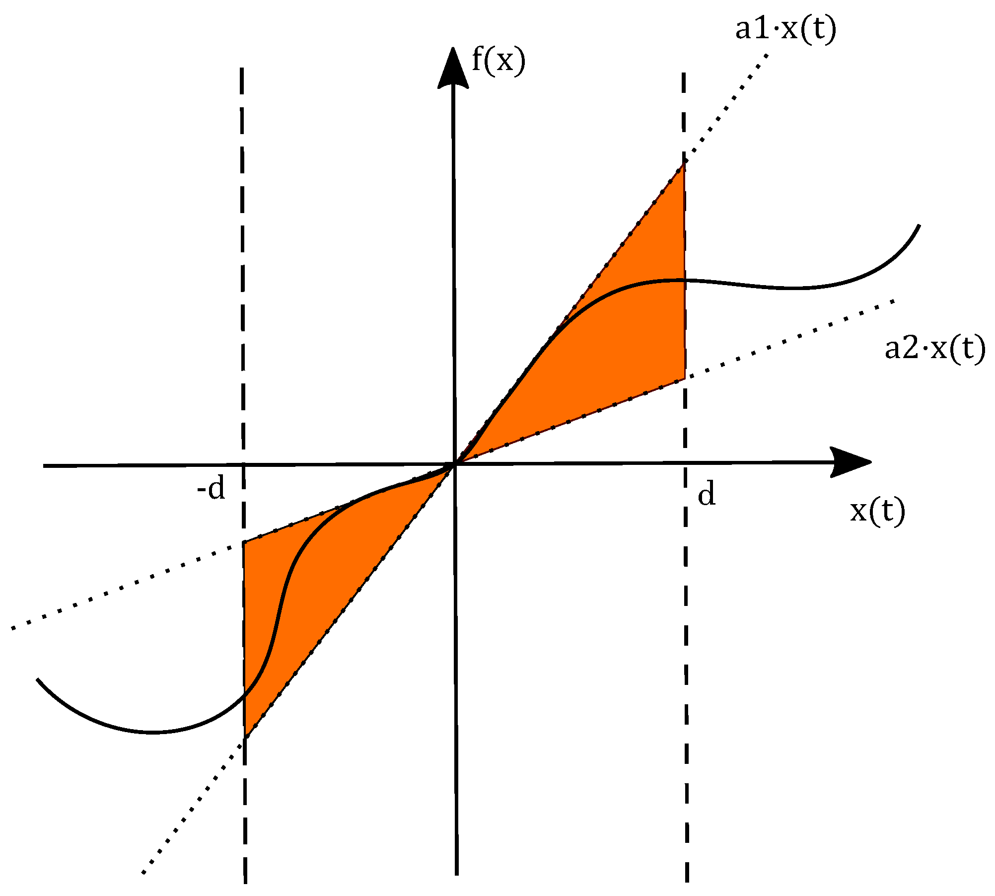
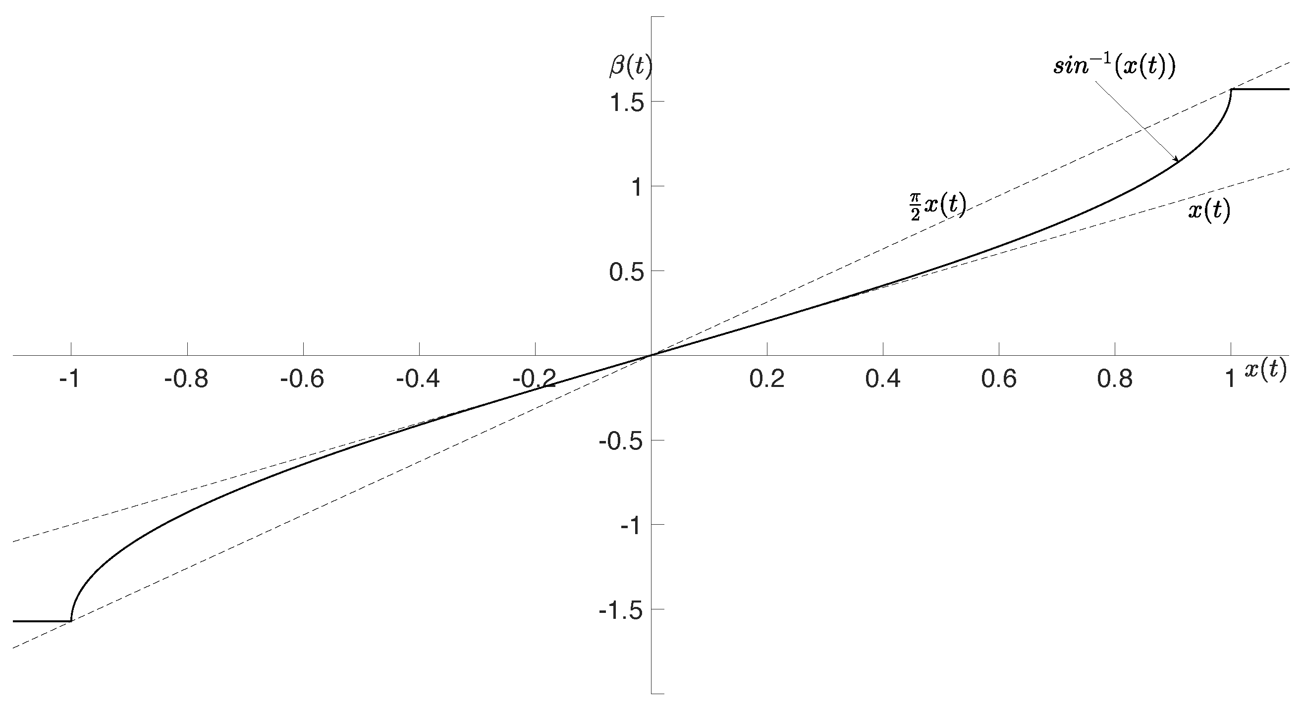
Sector non-linearity in fuzzy model construction appears in page 10 of [3], and is based on the following idea. We consider a non-linear system with a static non-linear term defined by function $f\left(x\right(t\left)\right)$. The aim is to find the global sector such that $f\left(x\right(t\left)\right)\in \left[a1a2\right]x\left(t\right)+\left[b1b2\right]$. Figure 2 illustrates this approach. Sometimes it is difficult to find global sectors for general non-linear functions. In this case, we can consider a local sector non-linearity where two vertical lines become this local sector where $-d<x\left(t\right)<d$, and where $[-dd]$ are the limits of variable $x\left(t\right)$ as illustrated in Figure 3.

Therefore, it is necessary to establish numerical limits $[-dd]$ of the variables to be approximated by the local sector non-linearity technique. In the case of a fixed-wing aircraft, those ranges include variables such as angle of attack, sideslip and airspeed. The information detailed in operational flight manuals or other technical information provided by aircraft designers [34,35] details the valid operational ranges as valuable sources to establish the particular value of limit $[-dd]$ for each variable.

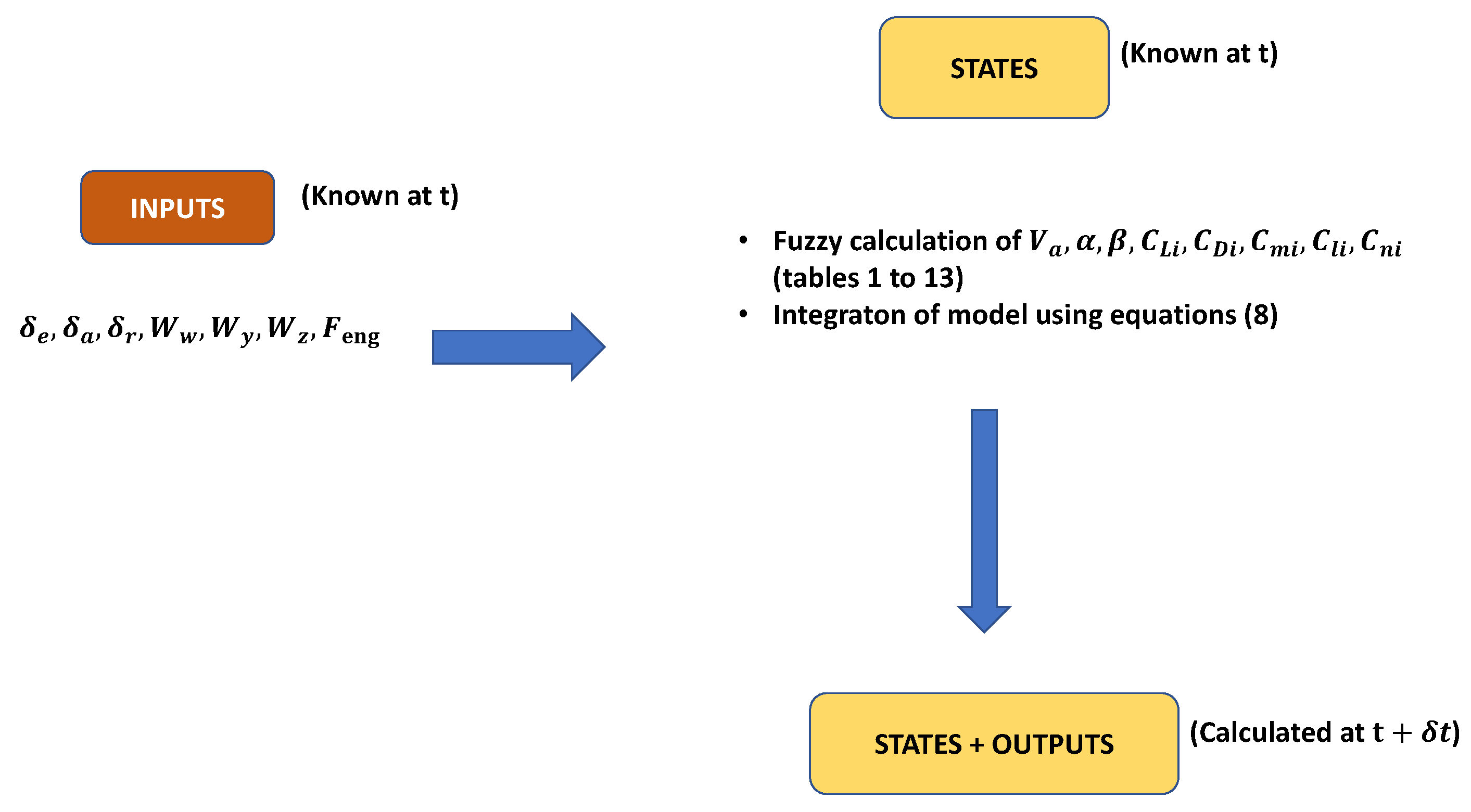
This approach is applied to obtain the fuzzy representation of static non-linear terms which appear in the model of fixed-wing aircraft according to Equation (1).

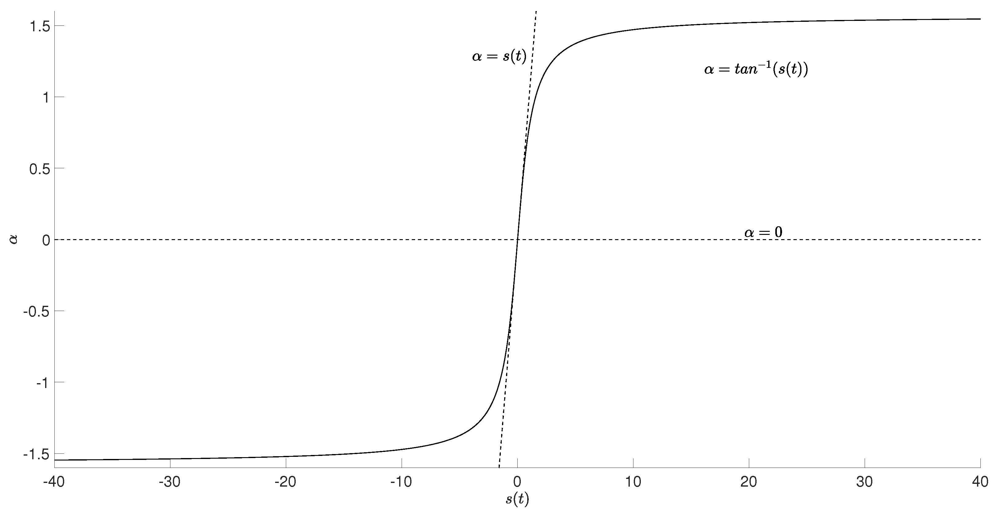
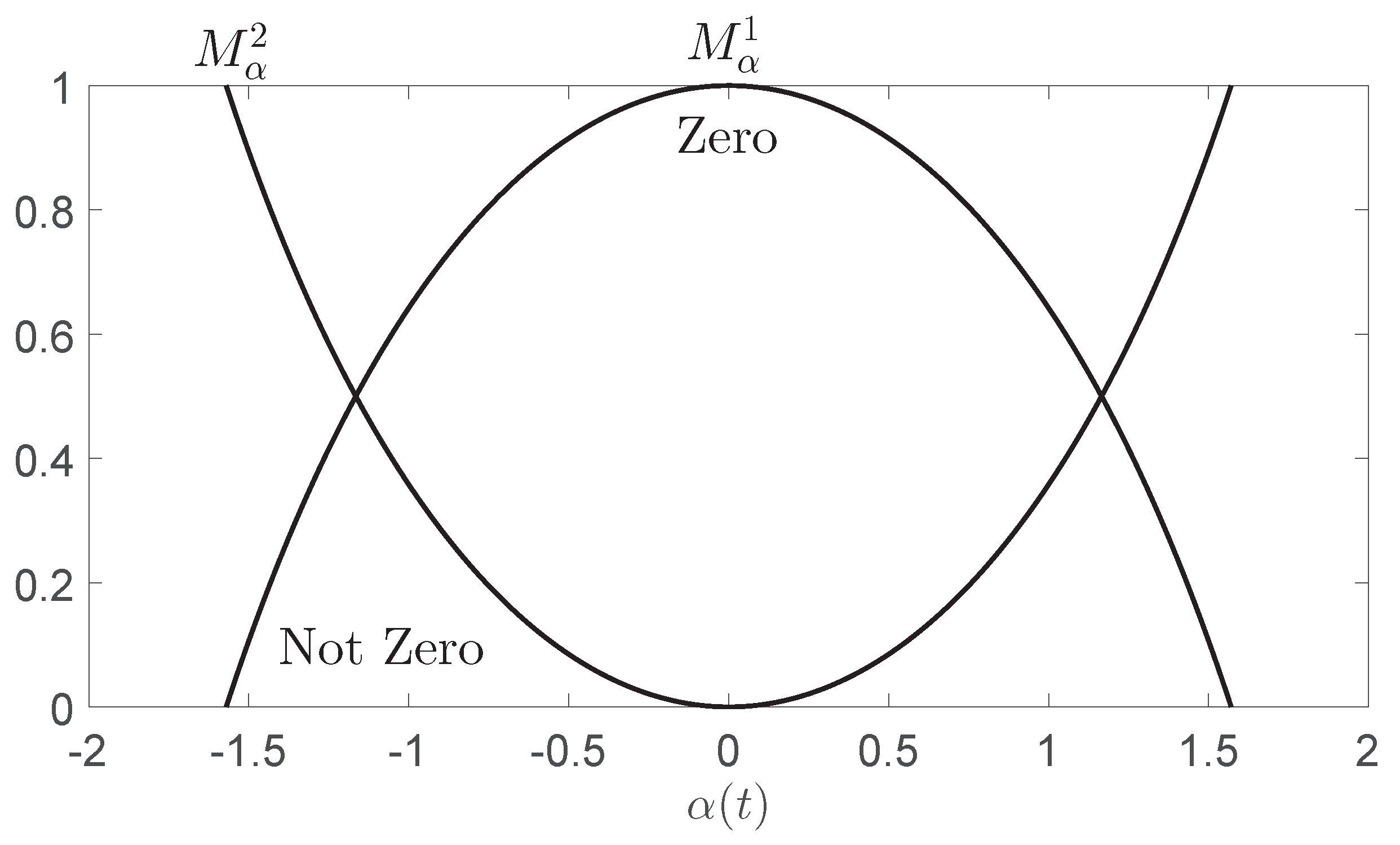
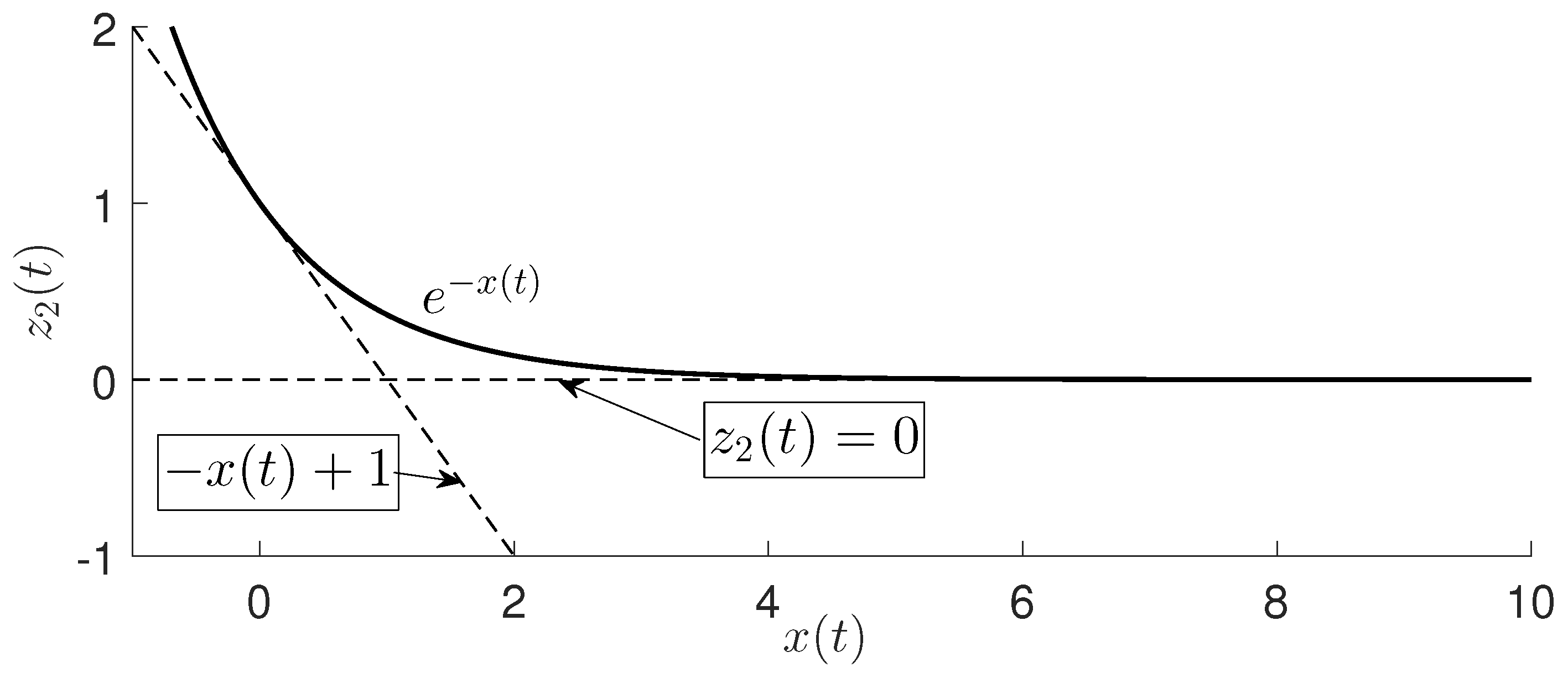
Example 1. 

The following non-linear function is the expression of angle-of-attack based on classic aircraft modeling:

$$\begin{array}{c}\alpha \left(t\right)={tan}^{-1}\left({\displaystyle \frac{x_1\left(t\right)}{x_2\left(t\right)}}\right)={tan}^{-1}\left(s\left(t\right)\right)\end{array}$$

(19)

$$\begin{array}{c}s\left(t\right)={\displaystyle \frac{x_1\left(t\right)}{x_2\left(t\right)}}\end{array}$$

(20)

We obtain a fuzzy representation in two steps. In the first step, we deal with the equation between α and s. Figure 4 shows the graphical representation of $\alpha \left(t\right)$ where two bounds of the global sector might be $[1,0]s\left(t\right)$. Therefore, based on these two simple sectors, $\alpha \left(t\right)$ can be represented using Equation (1) with two rules:

$$\alpha \left(t\right)=M_{\alpha }^{1}s\left(t\right)+M_{\alpha }^{2}0$$

(21)

where

$$M_{\alpha }^1+M_{\alpha }^2=1$$

(22)

The $M_{\alpha }^1$ and $M_{\alpha }^2$ consequents are $s\left(t\right)$ and 0; then,

$$\begin{array}{c}{A}_{\alpha }^1\left(t\right)=s\left(t\right),A_{\alpha }^2\left(t\right)=0\end{array}$$

(23)

Moreover, $\alpha \left(t\right)$ is the reference variable of the fuzzy model. Note that the membership function is dependent on $\alpha \left(t\right)$; then, it is important to remark that in this function, $s\left(t\right)=tan\left(\alpha \right(t\left)\right)$. Therefore, the membership functions can be calculated as

$$M_{\alpha }^1=\frac{\alpha \left(t\right)}{tan\left(\alpha \right(t\left)\right)},M_{\alpha }^2=1-M_{\alpha }^1=\frac{tan\left(\alpha \right(t\left)\right)-\alpha \left(t\right)}{tan\left(\alpha \right(t\left)\right)}$$

(24)

It should be noted that, in general, $s\ne 0$, but if this happens, we set $M_{\alpha }^1=1$ and $M_{\alpha }^2=0$. For the rest of the paper, these membership functions $M_k^i$ are termed Type I.

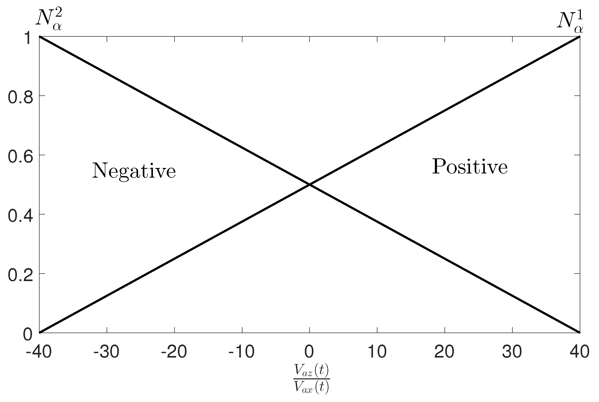
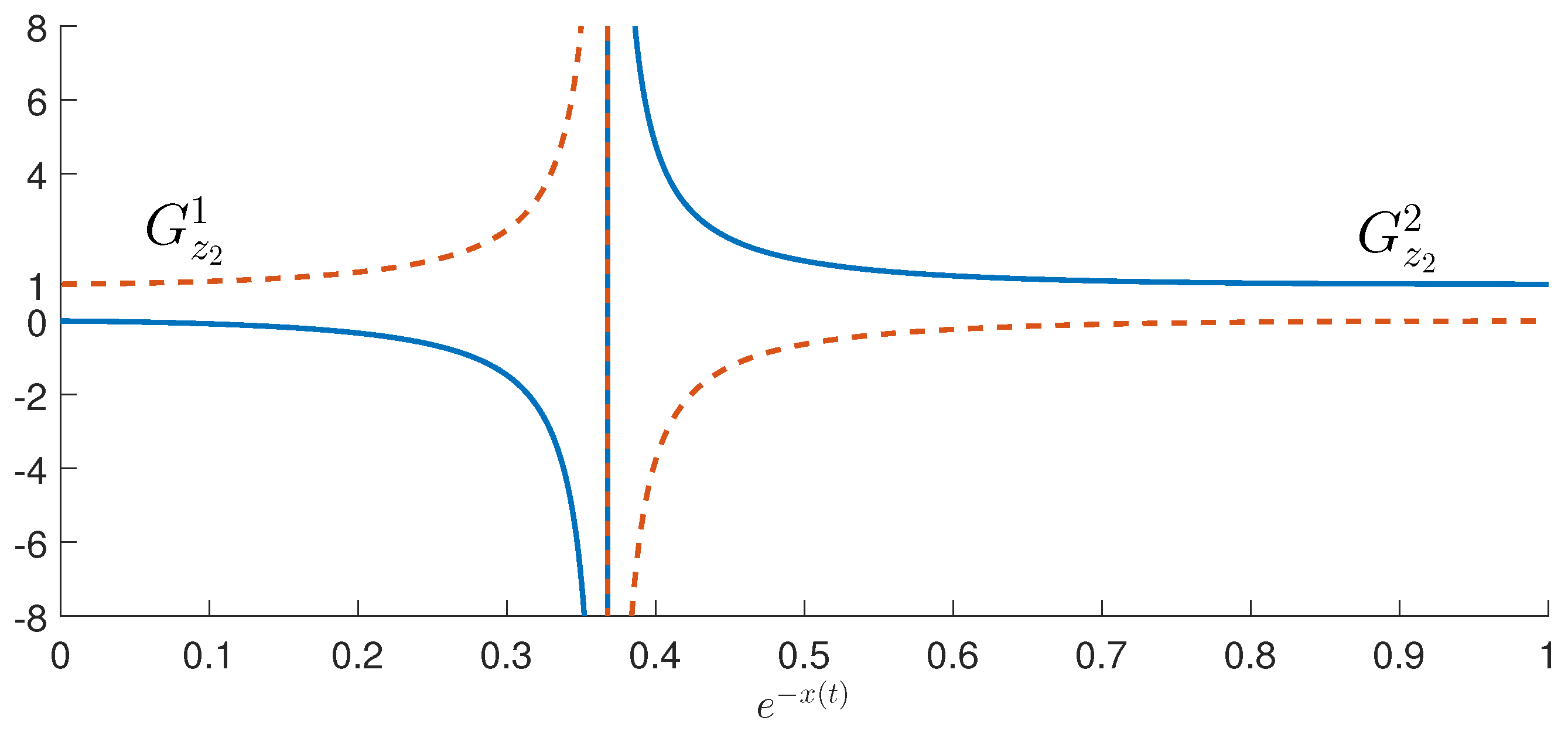
In the second step, we consider $s\left(t\right)$. In the angle-of-attack case, $s=\frac{x_1}{x_2}$ where $x_1\left(t\right)=V_{az}\left(t\right)$ and $x_2\left(t\right)=V_{ax}\left(t\right)$. In this non-linear case, the global sector cannot be defined, so a local sector isused instead, where the quotient is bounded by $\left[{\left(\frac{x_1}{x_2}\right)}_{min},{\left(\frac{x_1}{x_2}\right)}_{max}\right]$.

The reason for these limits is the same as that mentioned at the beginning of Example 1. The outcome of the local sector non-linearity is this fuzzy quantity with two rules:

$$s\left(t\right)=\frac{x_1\left(t\right)}{x_2\left(t\right)}=N_{\alpha }^1{\left(\frac{x_1}{x_2}\right)}_{max}+N_{\alpha }^2{\left(\frac{x_1}{x_2}\right)}_{min}$$

(25)

where membership functions are

$$\begin{array}{c}{N}_{\alpha }^1=\frac{\frac{x_1\left(t\right)}{x_2\left(t\right)}-{\left(\frac{x_1}{x_2}\right)}_{min}}{{\left(\frac{x_1}{x_2}\right)}_{max}-{\left(\frac{x_1}{x_2}\right)}_{min}}\\ N_{\alpha }^2=\frac{{\left(\frac{x_1}{x_2}\right)}_{max}-\frac{x_1\left(t\right)}{x_2\left(t\right)}}{{\left(\frac{x_1}{x_2}\right)}_{max}-{\left(\frac{x_1}{x_2}\right)}_{min}}\end{array}$$

(26)

In this case, the $N_{\alpha }^1$ and $N_{\alpha }^2$ consequents are ${\left(\frac{x_1}{x_2}\right)}_{max}$ and ${\left(\frac{x_1}{x_2}\right)}_{min}$; then,

$$\begin{array}{c}{A}_s^1\left(t\right)={\left(\frac{x_1}{x_2}\right)}_{max},A_s^2\left(t\right)={\left(\frac{x_1}{x_2}\right)}_{min}\end{array}$$

(27)

All membership functions with this structure are defined as type IV and labelled as $N_k^i$.

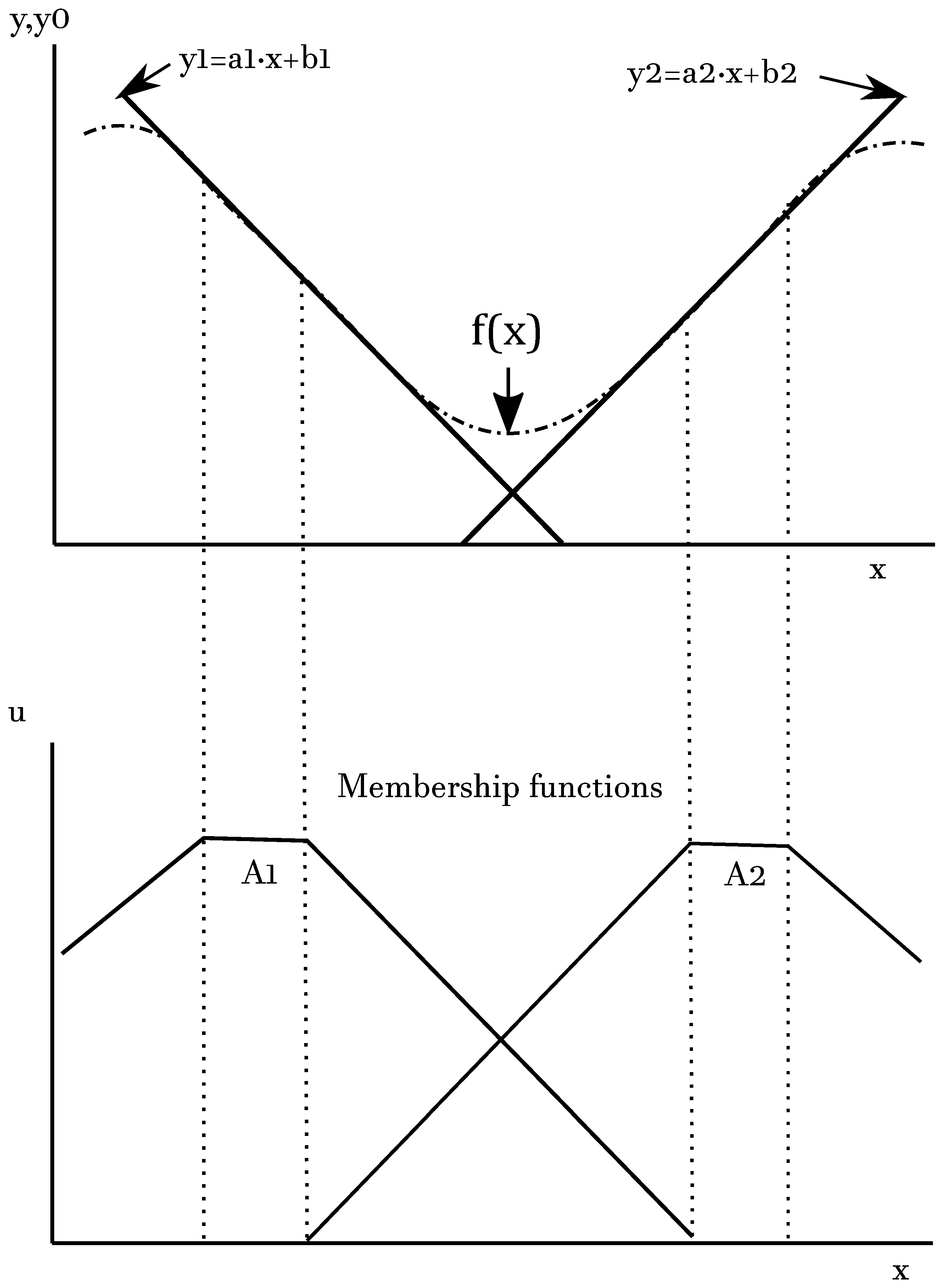
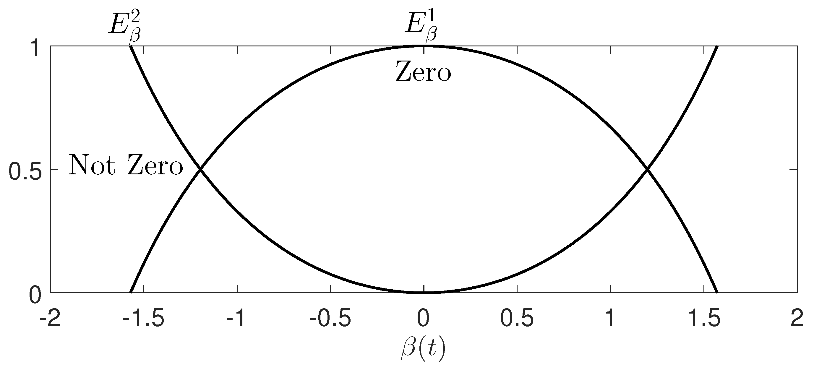
For representing the $\alpha \left(t\right)$ fuzzy model, the chosen value limits were $\frac{x_1}{x_2}=\frac{V_{az}\left(t\right)}{V_{ax}\left(t\right)}\in [-40,40]$. In fuzzy models, it is usual to name the membership functions as “Positive”, “Negative”, “Zero” and “Not Zero” (see Figure 5 and Figure 6). Finally, the fuzzy model for $\alpha \left(t\right)$ model has four rules after combining fuzzy Euantities (23) and (27), and it is presented in

Table 1. $\alpha$ Fuzzy Model.

Model Rule 1	Model Rule 2
IF $\alpha \left(t\right)$ is “Zero” and	IF $\alpha \left(t\right)$ is “Zero” and
$\frac{V_{az}\left(t\right)}{V_{ax}\left(t\right)}$ is “Positive”	$\frac{V_{az}\left(t\right)}{V_{ax}\left(t\right)}$ is “Negative”
THEN $\alpha \left(t\right)=A_{\alpha }^1$	THEN $\alpha \left(t\right)=A_{\alpha }^2$
Model Rule 3	Model Rule 4
IF $\alpha \left(t\right)$ is “Not zero” and	IF $\alpha \left(t\right)$ is “Not Zero” and
$\frac{V_{az}\left(t\right)}{V_{ax}\left(t\right)}$ is “Positive”	$\frac{V_{az}\left(t\right)}{V_{ax}\left(t\right)}$ is “Negative”
THEN $\alpha \left(t\right)=A_{\alpha }^3$	THEN $\alpha \left(t\right)=A_{\alpha }^4$

, where

$A_{\alpha }^1$	=	${s|}_{s={\left(\frac{V_{az}}{V_{ax}}\right)}_{max}}$	=	40
$A_{\alpha }^2$	=	${s|}_{s={\left(\frac{V_{az}}{V_{ax}}\right)}_{min}}$	=	$-40$
$A_{\alpha }^3$	=	0
$A_{\alpha }^4$	=	0

The defuzzification is carried out as

$$\alpha \left(t\right)=\sum _{j=1}^4{h}_j{A}_{\alpha }^j$$

(28)

where $h_1=M_{\alpha }^1{N}_{\alpha }^1$, $h_2=M_{\alpha }^1{N}_{\alpha }^2$, $h_3=M_{\alpha }^2{N}_{\alpha }^1$, $h_4=M_{\alpha }^2{N}_{\alpha }^2$. This fuzzy model is of the zero order because all the consequents are constants.

For further information regarding this example, see Example 3 in page 14 of [3].

4. Aircraft Fuzzy Model

As shown in Section 2.2, there is a large number of non-linear terms associated with aircraft dynamics. As a consequence, these terms are the main objective for applying the sector non-linearity methodology. Here, we provide a brief definition of all the types of membership functions and their consequent use following a similar procedure to Example 1 with membership Types I and IV. The different types on membership functions are chosen on the basis of the different structures of the most repeated non-linear terms.

4.1. Types of Membership Functions

Example 1 introduces membership Types I and IV, and following the same structure, this section describes Types II, III, V, VI and VII.

4.1.1. Type II: $\beta ={sin}^{-1}\left(x\left(t\right)\right)$

As it can be observed in Figure 7, the function can be delimited by the global sector as $\beta ={sin}^{-1}\left(x\left(t\right)\right)\in [\frac{\pi }{2},1]x\left(t\right)$. The global sector non-linearity method results in the following membership functions of Type II as illustrated in Figure 8:

$$\begin{array}{ccc}{E}_{\beta }^1=\frac{\beta \left(t\right)-sin\left(\beta \right(t\left)\right)}{sin\left(\beta \left(t\right)\right)(\frac{\pi }{2}-1)}& and& E_{\beta }^2=\frac{\frac{\pi }{2}sin\left(\beta \left(t\right)\right)-\beta \left(t\right)}{sin\left(\beta \left(t\right)\right)(\frac{\pi }{2}-1)}\end{array}$$

(29)

where $\frac{\pi }{2}x\left(t\right)$ and $x\left(t\right)$ are their consequents respectively. Consequently, this fuzzy model is of the first order.

4.1.2. Type III: $z_1\left(t\right)=\sqrt{x\left(t\right)}$

This non-linear term appears in Equations (14) and (15). In this particular case, a local sector non-linearity is applied, where bounds are defined as $[x_{min},x_{max}]$. Due to the non-negative value for the function, $x_{min}$ must be forced to 0. The membership functions can be defined as follows:

$$\begin{array}{ccc}{F}_{z_1}^1=\frac{\sqrt{x\left(t\right)}}{x_{max}}& and& F_{z_1}^2=\frac{x_{max}-\sqrt{x\left(t\right)}}{x_{max}}\end{array}$$

(30)

where $F_{z_1}^1$ and $F_{z_1}^2$ consequents are $x_{max}$ and $x_{min}=0$ respectively.

4.1.3. Type V: $z_2\left(t\right)=e^{-x\left(t\right)}$

To understand the fuzzy model from this type of equation, we consider that the exponential functions are used to model the aircraft ground effect. For this reason, variable $x\left(t\right)$ that expresses the distance of the aircraft from the ground will never be negative. Therefore, the minimum value will be $x\left(t\right)=0$, offering the maximum of function $z_2\left(t\right)=1$. In consequence, the first local sector is given by the $-x\left(t\right)+1$ line equation. The other global sector is defined by its asymptote when $x\left(t\right)$ reaches high values, and when it is placed at $z_2=0$. This global sector non-linearity is illustrated in Figure 9. The membership functions of Type V are described in the following Equations:

$$G_{z_2}^1=\frac{e^{-x\left(t\right)}}{1-x\left(t\right)},G_{z_2}^2=\frac{1-x\left(t\right)-e^{-x\left(t\right)}}{1-x\left(t\right)}$$

(31)

where $G_{z_2}^1$ and $G_{z_2}^2$ consequents are $1-x\left(t\right)$ and 0, respectively. The membership functions are illustrated in Figure 10.

4.1.4. Particularities of Type IV

Example 1 describes the membership function of quotient input terms as $\frac{x_1\left(t\right)}{x_2\left(t\right)}$. These functions are denoted as $N_k^i$ and are used in further membership structures. First, in quadratic terms ($x{\left(t\right)}^2$), where the membership function structure is equivalent to type IV, their consequents are $x_{max}$ and $x_{min}$, respectively. The linear equation terms also use the $N_k^i$ form, and its consequents are $a{x}_{max}+b$ and $a{x}_{min}+b$, respectively. For better understanding, in the summary

Table 2. $\beta \left(t\right)$ Fuzzy Model.

Function: $arcsin\left(\frac{V_{ay}\left(t\right)}{V_a\left(t\right)}\right)$,	Membership function types: II and IV
Max and Min: ${\left(\frac{V_{ay}}{V_a}\right)}_{max}=1$ and ${\left(\frac{V_{ay}}{V_a}\right)}_{min}=-1$
Model Rule 1	Model Rule 2
IF $\beta \left(t\right)$ is $E_{\beta }^1$ and $\frac{V_{ay}\left(t\right)}{V_a\left(t\right)}$ is $N_{\beta }^1$	IF $\beta \left(t\right)$ is $E_{\beta }^1$ and $\frac{V_{ay}\left(t\right)}{V_a\left(t\right)}$ is $N_{\beta }^2$
THEN $\beta \left(t\right)=A_{\beta }^1=\frac{\pi }{2}$	THEN $\beta \left(t\right)=A_{\beta }^2=-\frac{\pi }{2}$
Model Rule 3	Model Rule 4
IF $\beta \left(t\right)$ is $E_{\beta }^2$ and $\frac{V_{ay}\left(t\right)}{V_a\left(t\right)}$ is $N_{\beta }^1$	IF $\beta \left(t\right)$ is $E_{\beta }^2$ and $\frac{V_{ay}\left(t\right)}{V_a\left(t\right)}$ is $N_{\beta }^2$
THEN $\beta \left(t\right)=A_{\beta }^3=1$	THEN $\beta \left(t\right)=A_{\beta }^4=-1$

and

Table 3. $V_a\left(t\right)$ Fuzzy Model.

Function: $\sqrt{V_{ax}{\left(t\right)}^2+V_{ay}{\left(t\right)}^2+V_{az}{\left(t\right)}^2}$,	Membership function types: III
Max and Min: ${(V_{ax}^2+V_{ay}^2+V_{az}^2)}_{max}$ and ${(V_{ax}^2+V_{ay}^2+V_{az}^2)}_{min}=0$
Model Rule 1	Model Rule 2
IF $V_{ax}{\left(t\right)}^2+V_{ay}{\left(t\right)}^2+V_{az}{\left(t\right)}^2$ is $F_{V_a}^1$	IF $V_{ax}{\left(t\right)}^2+V_{ay}{\left(t\right)}^2+V_{az}{\left(t\right)}^2$ is $F_{V_a}^2$
THEN $V_a\left(t\right)=A_{V_a}^1={(V_{ax}^2+V_{ay}^2+V_{az}^2)}_{max}$	THEN $V_a\left(t\right)=A_{V_a}^2=0$

, the membership function for quadratic terms is $H_k^i$ (Type VI) and for linear functions, it is $J_k^i$ (Type VII).

4.2. Fuzzy Application to the Aaircraft Model

Once the different fuzzy model types are defined, the aircraft dynamic model introduced in Equations (8)–(18) can be reformulated in terms of fuzzy logic. In this new structure, the non-linear terms (except the polynomial forms) can be found in two sets of equations: the wind effects and aerodynamic coefficients.

4.2.1. Wind Effects

The variables included in non-linear terms and related to wind effects are $\alpha \left(t\right)$, $\beta \left(t\right)$ and $V_a\left(t\right)$. The  fuzzy model of the angle of attack, $\alpha \left(t\right)$, is described in Table 1, the  fuzzy model of the sideslip angle, $\beta \left(t\right)$, in Table 2, and the fuzzy model of the true airspeed, $V_a\left(t\right)$, in Table 3.

4.2.2. Aerodynamic Coefficients

The non-linear terms of the aerodynamic coefficients are reformulated here using the sector non-linearity method. In particular, Equation (28) introduces non-linear terms $C_{Li}$, $C_{Di}$, $C_{li}$, $C_{mi}$ and $C_{ni}$ where i refers the specific coefficient sub-term from the $C_L$, $C_D$, $C_l$, $C_m$ and $C_n$ aerodynamic coefficients, where      

$$\begin{array}{ccc}{C}_{L1}& =& \frac{\overline{c}}{V_a\left(t\right)}{C}_{Lq}q\left(t\right)\\ C_{L2}& =& C_{LH}{e}^{-{\lambda }_L{H}_{LG}\left(t\right)}\\ C_{D2}& =& C_{D\alpha 2}\alpha {\left(t\right)}^2\\ C_{l1}& =& \frac{\overline{c}}{V_a\left(t\right)}{C}_{lp}p\left(t\right)\\ C_{l2}& =& \frac{\overline{c}}{V_a\left(t\right)}r\left(t\right)(C_{lr0}+C_{lr\alpha }\alpha \left(t\right))\\ C_{m1}& =& \frac{\overline{c}}{V_a\left(t\right)}{C}_{mq}q\left(t\right)\\ C_{m2}& =& (C_{mH0}+C_{mH\alpha }\alpha \left(t\right))e^{-{\lambda }_m{H}_{LG}\left(t\right)}\\ C_{n1}& =& \frac{\overline{c}}{V_a\left(t\right)}{C}_{nr}r\left(t\right)\\ C_{n2}& =& \frac{\overline{c}}{V_a\left(t\right)}p\left(t\right)(C_{np0}+C_{np\alpha }\alpha \left(t\right))\\ C_{n3}& =& (C_{n{\beta }_0}+C_{n{\beta }_{\alpha }}\alpha \left(t\right))\beta \left(t\right)\end{array}$$

(32)

The aerodynamic coefficients in (32) are a combination of different non-linear functions of the types previously described. The fuzzy models of the ten aerodynamic coefficients are described in

Table 4. $C_{L1}$ Fuzzy Model.

Function: $C_{L1}\frac{\overline{c}}{V_a\left(t\right)}{C}_{Lq}q\left(t\right)$,	Membership function types: IV
Max and Min: ${\left(\frac{q}{V_a}\right)}_{max}$ and ${\left(\frac{q}{V_a}\right)}_{min}$
Model Rule 1	Model Rule 2
IF $\frac{q\left(t\right)}{V_a\left(t\right)}$ is $N_{C_{L1}}^1$	IF $\frac{q\left(t\right)}{V_a\left(t\right)}$ is $N_{C_{L1}}^2$
THEN $C_{L1}=A_{C_{L1}}^1=\overline{c}{C}_{Lq}{\left(\frac{q}{V_a}\right)}_{max}$	THEN $C_{L1}=A_{C_{L1}}^2=\overline{c}{C}_{Lq}{\left(\frac{q}{V_a}\right)}_{min}$

,

Table 5. $C_{L2}$ Fuzzy Model.

Function: $C_{L2}=C_{LH}{e}^{-{\lambda }_L{H}_{LG}\left(t\right)}$,	Membership function types: V
Max and Min: ${\lambda }_L{\left(H_{LG}\right)}_{max}$ and ${\lambda }_L{\left(H_{LG}\right)}_{min}=0$
Model Rule 1	Model Rule 2
IF ${\lambda }_L{H}_{LG}\left(t\right)$ is $G_{C_{L2}}^1$	IF ${\lambda }_L{H}_{LG}\left(t\right)$ is $G_{C_{L2}}^2$
THEN $C_{L2}=A_{C_{L2}}^1=C_{LH}(-{\lambda }_L{H}_{LG}\left(t\right)+1)$	THEN $C_{L2}=A_{C_{L2}}^2=0$

,

Table 6. $C_{D2}$ Fuzzy Model.

Function: $C_{D2}=C_{D\alpha 2}\alpha {\left(t\right)}^2$,	Membership function types: VI
Max and Min: ${\alpha }_{max}$ and ${\alpha }_{min}$
Model Rule 1	Model Rule 2
IF $\alpha \left(t\right)$ is $H_{C_{D2}}^1$	IF $\alpha \left(t\right)$ is $H_{C_{D2}}^2$
THEN $C_{D2}=A_{C_{D2}}^1=C_{D\alpha 2}{\alpha }_{max}\alpha \left(t\right)$	THEN $C_{L2}=A_{C_{L2}}^2=C_{D\alpha 2}{\alpha }_{min}\alpha \left(t\right)$

,

Table 7. $C_{l1}$ Fuzzy Model.

Function: $C_{l1}=\frac{\overline{c}}{V_a\left(t\right)}{C}_{lp}p\left(t\right)$,	Membership function types: IV
Max and Min: ${\left(\frac{p}{V_a}\right)}_{max}$ and ${\left(\frac{p}{V_a}\right)}_{min}$
Model Rule 1	Model Rule 2
IF $\frac{p\left(t\right)}{V_a\left(t\right)}$ is $N_{C_{l1}}^1$	IF $\frac{p\left(t\right)}{V_a\left(t\right)}$ is $N_{C_{l1}}^2$
THEN $C_{l1}=A_{C_{l1}}^1=\overline{c}{C}_{lp}{\left(\frac{p}{V_a}\right)}_{max}$	THEN $C_{l1}=A_{C_{L1}}^2=\overline{c}{C}_{lp}{\left(\frac{p}{V_a}\right)}_{min}$

,

Table 8. $C_{l2}$ Fuzzy Model.

Function: $C_{l2}=\frac{\overline{c}}{V_a\left(t\right)}r\left(t\right)(C_{lr0}+C_{lr\alpha }\alpha \left(t\right))$

Membership function types: IV and VII

Max and Min: ${\left(\frac{r}{V_a}\right)}_{max}$ and ${\left(\frac{r}{V_a}\right)}_{min}$ | ${\alpha }_{max}$ and ${\alpha }_{min}$

Model Rule 1

IF $\frac{r\left(t\right)}{V_a\left(t\right)}$ is $N_{C_{l2}}^1$ and $\alpha \left(t\right)$ is $J_{C_{l2}}^1$

THEN $C_{l2}=A_{C_{l2}}^1={\left(\frac{r}{V_a}\right)}_{max}(C_{lr0}+C_{lr\alpha }{\alpha }_{max})$

Model Rule 2

IF $\frac{r\left(t\right)}{V_a\left(t\right)}$ is $N_{C_{l2}}^1$ and $\alpha \left(t\right)$ is $J_{C_{l2}}^2$

THEN $C_{l2}=A_{C_{l2}}^2={\left(\frac{r}{V_a}\right)}_{max}(C_{lr0}+C_{lr\alpha }{\alpha }_{min})$

Model Rule 3

IF $\frac{r\left(t\right)}{V_a\left(t\right)}$ is $N_{C_{l2}}^2$ and $\alpha \left(t\right)$ is $J_{C_{l2}}^1$

THEN $C_{l2}=A_{C_{l2}}^3={\left(\frac{r}{V_a}\right)}_{min}(C_{lr0}+C_{lr\alpha }{\alpha }_{max})$

Model Rule 4

IF $\frac{r\left(t\right)}{V_a\left(t\right)}$ is $N_{C_{l2}}^2$ and $\alpha \left(t\right)$ is $J_{C_{l2}}^2$

THEN $C_{l2}=A_{C_{l2}}^4={\left(\frac{r}{V_a}\right)}_{min}(C_{lr0}+C_{lr\alpha }{\alpha }_{min})$

,

Table 9. $C_{m1}$ Fuzzy Model.

Function: $C_{m1}=\frac{\overline{c}}{V_a\left(t\right)}{C}_{mq}q\left(t\right)$,	Membership function types: IV
Max and Min: ${\left(\frac{q}{V_a}\right)}_{max}$ and ${\left(\frac{q}{V_a}\right)}_{min}$
Model Rule 1	Model Rule 2
IF $\frac{q\left(t\right)}{V_a\left(t\right)}$ is $N_{C_{m1}}^1$	IF $\frac{q\left(t\right)}{V_a\left(t\right)}$ is $N_{C_{m1}}^2$
THEN $C_{m1}=A_{C_{m1}}^1=\overline{c}{C}_{mq}{\left(\frac{q}{V_a}\right)}_{max}$	THEN $C_{m1}=A_{C_{m1}}^2=\overline{c}{C}_{mq}{\left(\frac{q}{V_a}\right)}_{min}$

,

Table 10. $C_{m2}$ Fuzzy Model.

Function: $C_{m2}=(C_{mH0}+C_{mH\alpha }\alpha \left(t\right))e^{-{\lambda }_m{H}_{LG}\left(t\right)}$

Membership function types: V and VII

Max and Min: ${\lambda }_m{H}_{LG,max}$ and ${\lambda }_m{H}_{LG,max}$ | ${\alpha }_{max}$ and ${\alpha }_{min}$

Model Rule 1

IF ${\lambda }_m{H}_{LG}\left(t\right)$ is $G_{C_{m2}}^1$ and $\alpha \left(t\right)$ is $J_{C_{m2}}^1$

THEN $C_{m2}=A_{C_{m2}}^1=(-{\lambda }_m{H}_{LG}\left(t\right)+1)(C_{mH0}+C_{mH\alpha }{\alpha }_{max})$

Model Rule 2

IF ${\lambda }_m{H}_{LG}\left(t\right)$ is $G_{C_{m2}}^1$ and $\alpha \left(t\right)$ is $J_{C_{m2}}^2$

THEN $C_{m2}=A_{C_{m2}}^2=(-{\lambda }_m{H}_{LG}\left(t\right)+1)(C_{mH0}+C_{mH\alpha }{\alpha }_{min})$

Model Rule 3

IF ${\lambda }_m{H}_{LG}\left(t\right)$ is $G_{C_{m2}}^2$ and $\alpha \left(t\right)$ is $J_{C_{m2}}^1$

THEN $C_{m2}=A_{C_{m2}}^3=0$

Model Rule 4

IF ${\lambda }_m{H}_{LG}\left(t\right)$ is $G_{C_{m2}}^2$ and $\alpha \left(t\right)$ is $J_{C_{m2}}^2$

THEN $C_{m2}=A_{C_{m2}}^4=0$

,

Table 11. $C_{n1}$ Fuzzy Model.

Function: $\frac{\overline{c}}{V_a\left(t\right)}{C}_{nr}r\left(t\right)$,	Membership function types: IV
Max and Min: ${\left(\frac{r}{V_a}\right)}_{max}$ and ${\left(\frac{r}{V_a}\right)}_{min}$
Model Rule 1	Model Rule 2
IF $\frac{r\left(t\right)}{V_a\left(t\right)}$ is $N_{C_{n1}}^1$	IF $\frac{r\left(t\right)}{V_a\left(t\right)}$ is $N_{C_{n1}}^2$
THEN $C_{n1}=A_{C_{n1}}^1=\overline{c}{C}_{nr}{\left(\frac{r}{V_a}\right)}_{max}$	THEN $C_{n1}=A_{C_{n1}}^2=\overline{c}{C}_{nr}{\left(\frac{r}{V_a}\right)}_{min}$

,

Table 12. $C_{n2}$ Fuzzy Model.

Function: $C_{n2}=\frac{\overline{c}}{V_a\left(t\right)}p\left(t\right)(C_{np0}+C_{np\alpha }\alpha \left(t\right))$

Membership function types: IV and VII

Max and Min: ${\left(\frac{p}{V_a}\right)}_{max}$ and ${\left(\frac{p}{V_a}\right)}_{min}$ | ${\alpha }_{max}$ and ${\alpha }_{min}$

Model Rule 1

IF $\frac{p\left(t\right)}{V_a\left(t\right)}$ is $N_{C_{n2}}^1$ and $\alpha \left(t\right)$ is $J_{C_{n2}}^1$

THEN $C_{n2}=A_{C_{n2}}^1={\left(\frac{p}{V_a}\right)}_{max}(C_{np0}+C_{np\alpha }{\alpha }_{max})$

Model Rule 2

IF $\frac{p\left(t\right)}{V_a\left(t\right)}$ is $N_{C_{n2}}^1$ and $\alpha \left(t\right)$ is $J_{C_{n2}}^2$

THEN $C_{n2}=A_{C_{n2}}^2={\left(\frac{p}{V_a}\right)}_{max}(C_{np0}+C_{np\alpha }{\alpha }_{min})$

Model Rule 3

IF $\frac{p\left(t\right)}{V_a\left(t\right)}$ is $N_{C_{n2}}^2$ and $\alpha \left(t\right)$ is $J_{C_{n2}}^1$

THEN $C_{n2}=A_{C_{n2}}^3={\left(\frac{p}{V_a}\right)}_{min}(C_{np0}+C_{np\alpha }{\alpha }_{max})$

Model Rule 4

IF $\frac{p\left(t\right)}{V_a\left(t\right)}$ is $N_{C_{n2}}^2$ and $\alpha \left(t\right)$ is $J_{C_{n2}}^2$

THEN $C_{n2}=A_{C_{l2}}^4={\left(\frac{p}{V_a}\right)}_{min}(C_{np0}+C_{np\alpha }{\alpha }_{min})$

and

Table 13. $C_{n3}$ Fuzzy Model.

Function: $C_{n3}=(C_{n{\beta }_0}+C_{n{\beta }_{\alpha }}\alpha \left(t\right))\beta \left(t\right)$

Membership function types: IV and VII

Max and Min: ${\beta }_{max}$ and ${\beta }_{min}$ | ${\alpha }_{max}$ and ${\alpha }_{min}$

Model Rule 1

IF $\beta \left(t\right)$ is $H_{C_{n3}}^1$ and $\alpha \left(t\right)$ is $J_{C_{n3}}^1$

THEN $C_{n3}=A_{C_{n3}}^1={\beta }_{max}(C_{n{\beta }_0}+C_{n{\beta }_{\alpha }}{\alpha }_{max})$

Model Rule 2

IF $\beta \left(t\right)$ is $H_{C_{n3}}^1$ and $\alpha \left(t\right)$ is $J_{C_{n3}}^2$

THEN $C_{n3}=A_{C_{n3}}^2={\beta }_{max}(C_{n{\beta }_0}+C_{n{\beta }_{\alpha }}{\alpha }_{min})$

Model Rule 3

IF $\beta \left(t\right)$ is $H_{C_{n3}}^2$ and $\alpha \left(t\right)$ is $J_{C_{n3}}^1$

THEN $C_{n3}=A_{C_{n3}}^3={\beta }_{min}(C_{n{\beta }_0}+C_{n{\beta }_{\alpha }}{\alpha }_{max})$

Model Rule 4

IF $\beta \left(t\right)$ is $H_{C_{n3}}^2$ and $\alpha \left(t\right)$ is $J_{C_{n3}}^2$

THEN $C_{n3}=A_{C_{n3}}^4={\beta }_{min}(C_{n{\beta }_0}+C_{n{\beta }_{\alpha }}{\alpha }_{min})$

. The maximums and minimums are left as unknown variables and the user should define them. This is because there are different bound conditions for each aircraft type and the objective of this paper is to propose a general model, that is to say, a full flight dynamics model for later application introducing all the aircraft constants.

Figure 11 presents the procedure to combine all the fuzzy models presented in Table 1, Table 2, Table 3, Table 4, Table 5, Table 6, Table 7, Table 8, Table 9, Table 10, Table 11, Table 12 and Table 13 for obtaining a full fuzzy model for the aircraft.

5. Results and Validation

Due to the complexity of the formulation presented in this work and the large number of fuzzy terms involved, the Fuzzy Modelling Toolbox for Aircraft Systems (FMA Toolbox) is developed in Matlab. The FMA Toolbox reformulates fixed-wing aircraft models in terms of fuzzy logic, and it can be downloaded at GitHub [36]. Furthermore, to clarify the set of functions and scripts developed in this Toolbox, the detailed user manual can be consulted in [37]. Also, the main implementation of the fuzzy non-linear model for fixed-wing aircraft can be found in [38], where Equations (2)–(18) (introduced in Section 2) are coded in terms of fuzzy logic. This toolbox uses Algorithm 1.

Algorithm 1 Aircraft fuzzy model

1: Set $t=0$. Set initial conditions of the model. 2: while $t\le t_{max}$ do 3:     Read the values of the inputs at t 4:     Compute non-linear terms at t using fuzzy models from Table 1, Table 2, Table 3, Table 4, Table 5, Table 6, Table 7, Table 8, Table 9, Table 10, Table 11, Table 12 and Table 13 5:     Substitute non-linear terms in aircraft model Equations (8). 6:     Integrate these equations and obtain all the states and outputs at $t+\delta t$ 7:     Set $t=t+\delta t$ 8: end while

5.1. Inputs and Initial Conditions

Once the classical aircraft model is completely reformulated in terms of fuzzy logic, it is necessary to test and compare the behavior of these two models using real data. The aircraft dynamic model used here is based on Onera’s benchmark of the landing challenge [31]. Thus, it is logical to put the initial values of this model into the fuzzy model.

Table 14. Airbus A310 parameters.

Mass and Geometry
S = 360 m2	$\overline{c}$ = $7.500$ m	$z_{eng}$ = 2 m	$m_0$ = $150,000$ kg	$I_{xx}$ = ${10}^7$ kg/m2
$I_{yy}$ = $1.600·{10}^7$ kg/m2	$I_{zz}$ = $2.400·{10}^7$ kg/m2	$I_{xz}$ = $-{10}^6$ kg/m2	$x_{CG}$ = 21 m
Aerodynamic Coefficients
$C_{L0}=0.900$	$C_{L\alpha }=5.500$	$C_{Lq}=3.300$	$C_{L\delta e}=0.320$	$C_{LH}=0.200$
${\lambda }_L=0.120$	$C_{D0}=0.065$	$C_{D\alpha }=0.400$	$C_{D\alpha 2}=1.550$	$C_{Y\beta }=-0.700$
$C_{Y\delta r}=0.250$	$C_{l\beta }=-3$	$C_{lp}=-15$	$C_{lr0}=5$	$C_{lr\alpha }=35$
$C_{\delta a}=-0.700$	$C_{l\delta r}=0.200$	$C_{m0}=-0.300$	$C_{m\alpha }=-1.500$	$C_{mq}=-12$
$C_{m\delta e}=-1.200$	$C_{mh0}=-0.090$	$C_{mh\alpha }=-0.900$	${\lambda }_m=0.150$	$C_{n\beta 0}=0.850$
$C_{n\beta \alpha }=-1.950$	$C_{np0}=-3$	$C_{np\alpha }=-35$	$C_{nr}=-7$	$C_{n\delta a}=-0.04$
$C_{n\delta r}=-1.250$

shows all the parameters of the Airbus A310 aircraft used here. It should be emphasized that the results are simulated in a short time frame and that is why the aircraft mass is considered constant, as well as the inertia matrix. The initial conditions of the simulation are calculated as classic Taylor series equilibrium points searching for the actuator trim values. For a more realistic model, these actuators are also modeled and their dynamics are approximated by magnitude and rate limit first-order filters whose characteristics are summarized in

Table 15. Engine and actuator characteristics.

Parameter	Time-Constant	Lower-Bound	Upper-Bound	Rate-Limit
Engines (EPR)	2 s	0.950	1.600	0.100
Ailerons (${\delta }_A$)	0.060 s	−55 deg	55 deg	60 deg/s
Elevators (${\delta }_E$)	0.070 s	−25 deg	25 deg	20 deg/s
Rudder ($\delta R$)	0.200 s	−30 deg	30 deg	30 deg/s

. To obtain significant simulation results, the actuators must vary with different combinations as shown in Figure 12. Finally, the fuzzy model needs maximum and minimum values to be defined.

Table 16. Fuzzy model limits.

Parameter	Lower-Bound	Upper-Bound	Unit
$\alpha$	$-{\displaystyle \frac{\pi }{2}}$	${\displaystyle \frac{\pi }{2}}$	rad
$\beta$	$-{\displaystyle \frac{\pi }{2}}$	${\displaystyle \frac{\pi }{2}}$	rad
${\displaystyle \frac{p}{V_a}}$	$-1$	1	rad/m
${\displaystyle \frac{q}{V_a}}$	$-1$	1	rad/m
${\displaystyle \frac{r}{V_a}}$	$-1$	1	rad/m
$V_a^2$	1	500	m2/s2
${\displaystyle \frac{V_{az}}{V_{ax}}}$	$-40$	40	(-)
${\displaystyle \frac{V_{ay}}{V_a}}$	$-1$	1	(-)
$H_{LG}$	0	40	m

defines very conservative limits; for example, $\alpha \left(t\right)$ and $\beta \left(t\right)$ are bounded by a very large interval. Therefore, it is important to remark that some of these value limits can be selected more restrictive, if desired.

5.2. Simulation Results

To compare the non-linear dynamic model of Civilian Aircraft Landing Challenge [31] and the fuzzy logic model, both models are simulated under equivalent conditions. Particularly, simulations are carried out using the Toolbox developed in [36]. These simulations are executed on a PC with Intel Core i5 CPU at 1.6 GHz with 16 GB of DDR3 RAM and using MATLAB 2020B. A computation time of 72 s is necessary to obtain the dynamic evolution of the simulation model for 100 s.

The original non-linear dynamical model developed in Equation (8) uses a first-order algorithm with a fixed time step of 0.05 seconds, usually known as ODE1 [39], to solve the differential equations. For that reason, to validate and compare the fuzzy model proposed with the original one in equivalent conditions, the Toolbox developed uses the same first-order approximation (ODE1) as a default. However, higher-order solvers, such as ODE2 or ODE3 [39], are available in the Toolbox and can used to simulate the aircraft fuzzy model, always using a fixed time step. Inn addition, the aircraft fuzzy model is simulated by applying Algorithm 1.

On the other hand, the Variance Accounted For (VAF) index is used to provide an objective value of the percent of similitude between the two output models [12]. The VAF is governed by the following equation:

$$VA{F}_i=\left(1-\frac{var(y_i-{\widehat{y}}_i)}{var\left(y_i\right)}\right)100\%,$$

(33)

where $y_i$ is the measured output (classic model) and ${\widehat{y}}_i$ is the estimated output (fuzzy model) for the ith component. Figure 13 and Figure 14 show the response of the state variables in both models. Note that the fuzzy modeling method is an exact method, and so the VAFs have high values. Nevertheless, the index is not 100% because the non-linear model of [31] uses the integration of the Euler angles while this integration is based on quaternions in the fuzzy model. In this simulation, the difference is insignificant due the short period of simulation. Therefore, the error increases as simulation time increases.

6. Conclusions and Future Works

A general framework for modelling fixed-wing aircraft using fuzzy structures and sector non-linearity techniques is proposed. The main contribution the obtention of a more general and accurate non-linear model than other alternatives proposed in the existing literature, such as [28,29]. Moreover, the approach presented allows for the expression of aerodynamic coefficients, moments, forces and wind effects, all of them expressed in terms of fuzzy logic and the body frame. This is possible thanks to the capability of the global and local sector non-linearity technique to approximate non-linear terms with fuzzy logic rules and with the same accuracy as the original non-linear model. In addition, the proposed quaternions form contributes to the good performance of the fuzzy logic model by removing discontinuities and more complex trigonometric functions. However, the good mathematical performance of the quaternions has the negative effect of losing the physical concept of comparing the Euler angles. Nevertheless, it is possible to find an equivalent Euler representation from quaternions.

The main limitation of obtaining the equivalent fuzzy model is the requirement to limit the maximum and minimum values for some of the system variables. This is due to the application of the local sector non-linearity technique, as detailed in Section 3 and Section 4. However, this limitation is not extremely constraining in the case of a fixed-wing aircraft, as there is often a significant amount of information available (theoretical and experimental) from manufacturers and the research community on the limits of these variables.

A Matlab toolbox is implemented [36] to simplify the application of this new approach for any standard fixed-wing aircraft defined by classical parameters such as geometry, mass, coefficients and bound conditions, where the outcome of the toolbox is a newly reformulated fuzzy model in terms of quaternions.

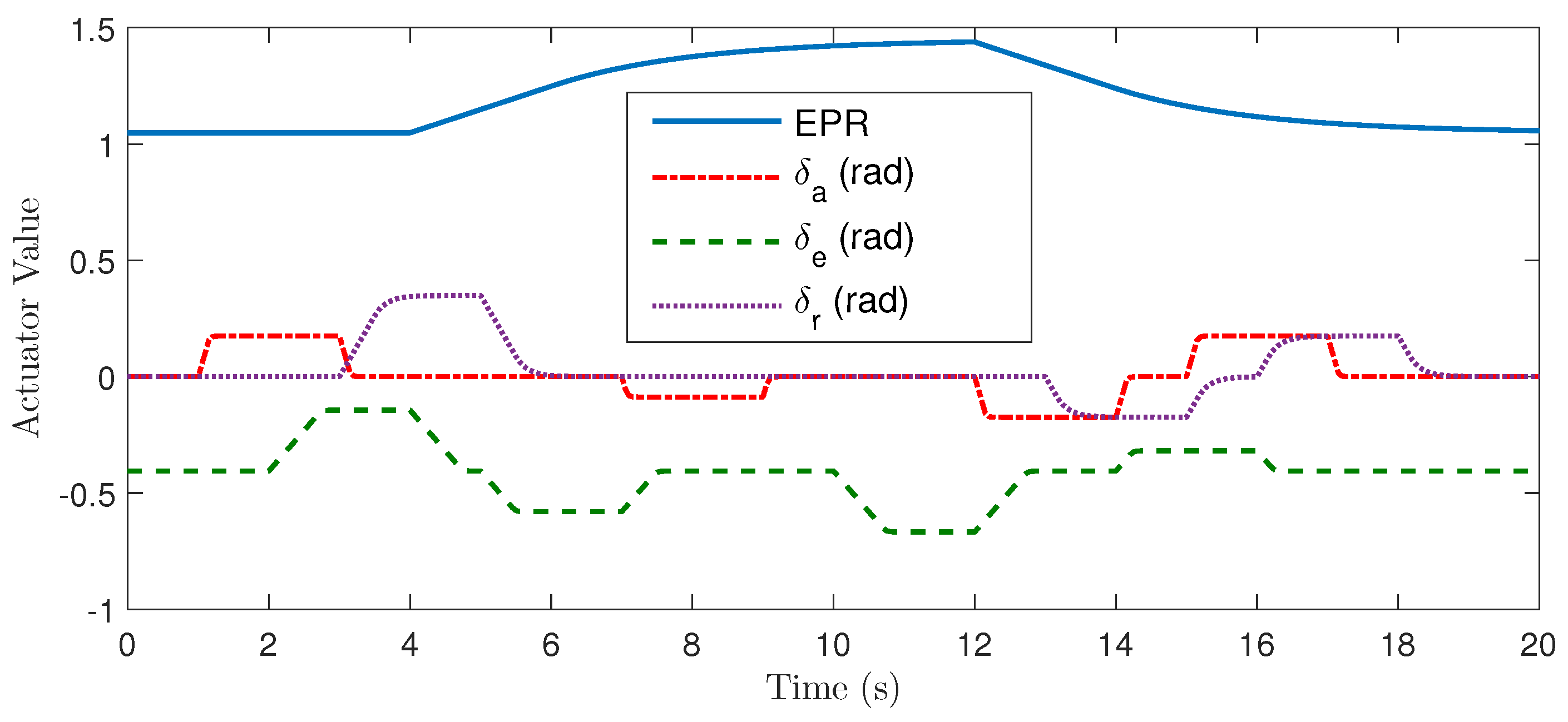
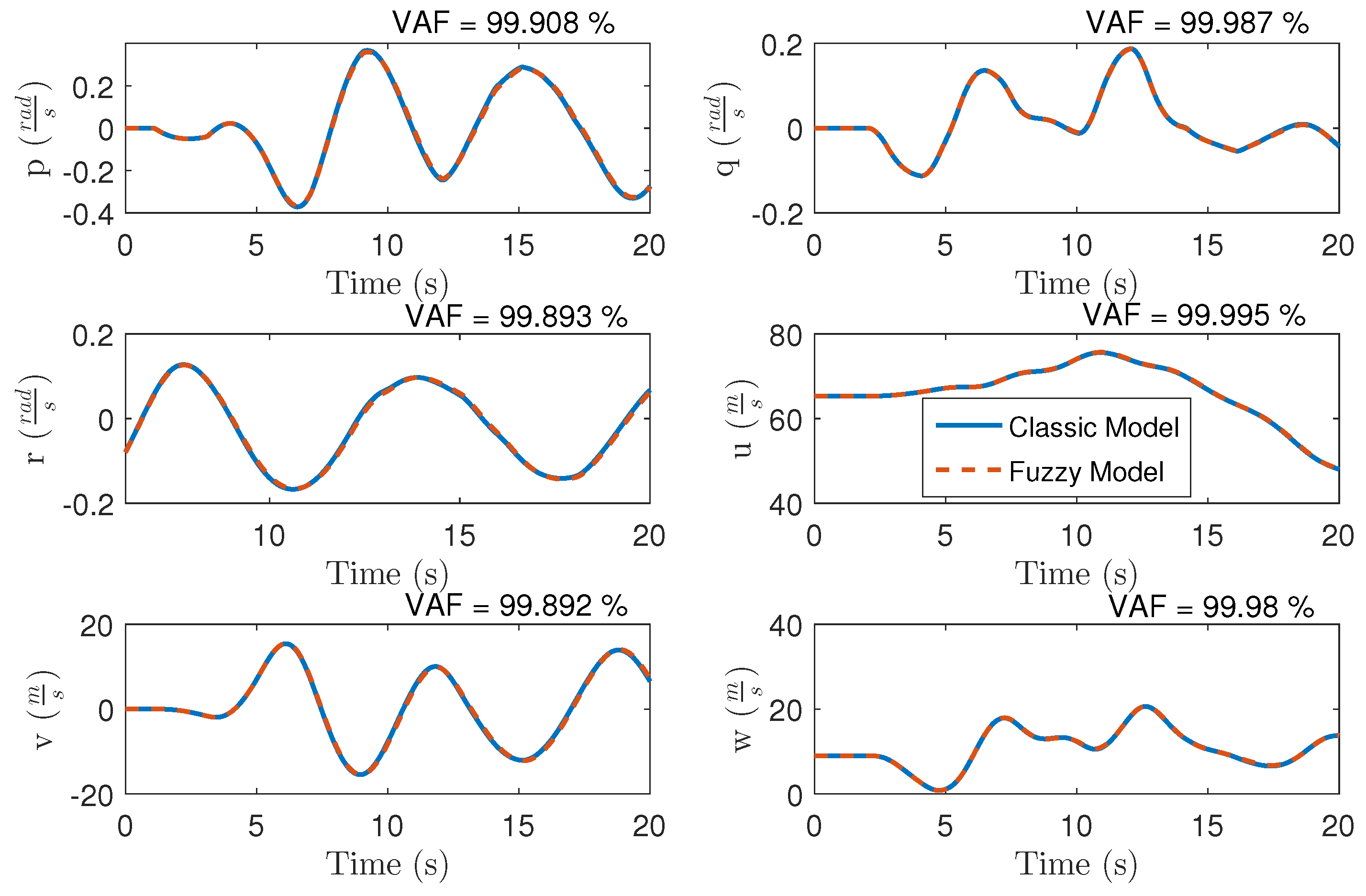
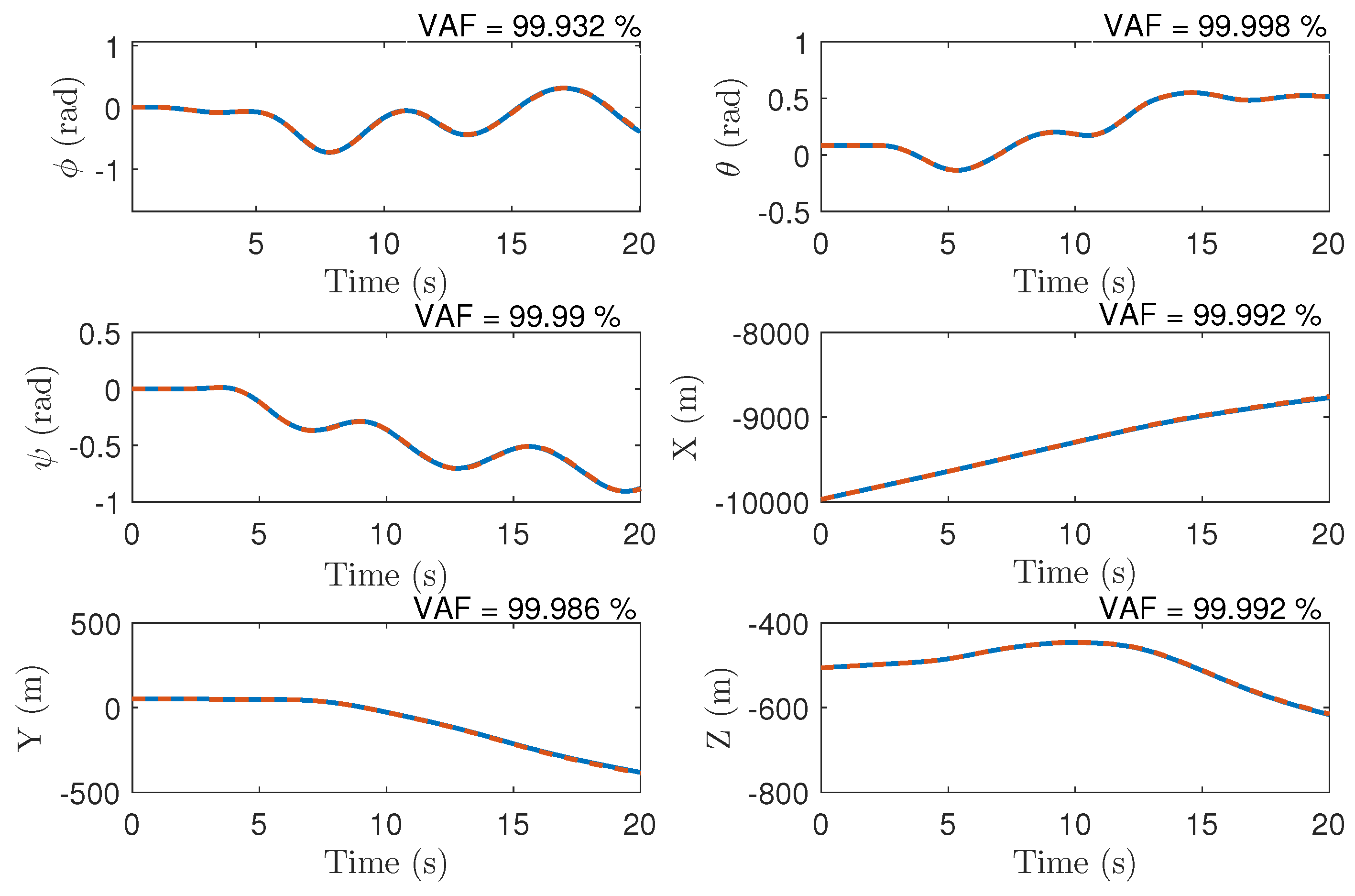
On the other hand, in Section 5, using this Matlab toolbox, a fuzzy equivalent model for the Onera non-linear model benchmark of the A310 [31] is obtained. Also, a comparison between the AIRBUS A310 model developed by ONERA and the obtained fuzzy model is performed. As a consequence, it is concluded that both models are equivalent.

The following research step consists of defining in terms of the Takagi–Sugeno structure (page 6 of [3]) the fuzzy model obtained in this work. This representation is suitable for designing PDC and non-PDC fuzzy controllers using well-known methodologies based on linear matrix inequalities [5,6,40].