1. Introduction
Advanced composite materials have been widely used in the primary load-bearing structures of civil aircraft. The study of the mechanical performance of damaged composite laminate panels and their repaired conditions is becoming increasingly important. Common damages in composite laminate panels of civil aircraft include delamination and debonding. One commonly used repair method for such damages is step scarf repair [
1,
2].
For classical laminate theory, the adoption of the straight normal assumption, ignoring the influence of deflection on transverse strain [
3,
4], results in a poor description of the response of structures with small span-to-height ratios. It becomes challenging to accurately calculate interlaminar out-of-plane stresses with nonlinear distribution along the thickness of small span-to-height ratio plates.
Three-dimensional solutions have emerged [
5,
6,
7,
8,
9] in order to overcome the defects in two-dimensional plane solutions. For the general three-dimensional displacement elements, refined mesh division in the thickness direction is required to improve the precision of the results. But in three-dimensional finite element solution methods, there can be discontinuities in the thickness direction when solving stress at nodes using the stress–strain relationship. In order to maximize the continuity and accuracy of stress, Hinton E [
10] employs the least squares method to address the numerical discontinuity problem when using finite element functions to handle physically continuous systems. Zienkiewicz O C [
11] uses a continuously expanded polynomial to establish a super convergent patch recovery method, and Boroomand B [
12] proposes a method based on balanced recovery stress based on Zienkiewicz O C’s work. Generally, mesh refinement or element enhancement methods can minimize such discontinuities and yield more accurate stress field predictions. It is worth noting that layer-wise mixed theory [
12,
13] can also address this issue. Recently, N. Magome [
14] proposed a novel strategy called a B-spline-based SFEM to cover the problems stated above; it can also handle the accuracy of numerical integration and matrix singularity.
The so-called H–R variational principle is a generalized functional proposed with displacement and stress as independent variables, and this state function includes three displacement variables and three stress variables. The main advantages of the semi-analytical solution method based on mixed elements for the above state space function are that the continuity of displacement and out-of-plane stress parameters can be ensured through transfer matrices, and the fulfillment of out-of-plane stress boundary conditions for components is easily achieved. K. Xia [
15] stated a semi-analytical method to determine a mixed-mode fracture resistance curve (R-curve) and mode mixture of ADCB composite laminates and verified its effectiveness and wide applicability. However, for commonly encountered large and complex engineering structures, the efficiency of the semi-analytical method is lower than that of traditional displacement methods. Additionally, for plates with non-uniform thickness, the semi-analytical method is not suitable for stress analysis. Furthermore, the semi-analytical method cannot guarantee each layer’s local continuity of in-plane stresses.
A 12-node partial hybrid model based on the H–R variational principle was proposed by Liao et al. [
8], where three displacement variables and two out-of-plane shear forces are treated as independent variables, and these five variables can be solved simultaneously. However, the above method cannot ensure the continuity of out-of-plane normal stresses between different layers and is not conducive to introducing boundary normal stress conditions. Consequently, K. Rah [
16] introduced a low-order partial hybrid stress solid-shell element based on the composite energy functional for the analysis of laminated composite structures; it can accurately calculate interlaminar stress through the element thickness.
The mixed element is a commonly used symmetric element in the H–R mixed variational principle. When used to solve various physical problems, it is generally non-positive definite due to the presence of zero elements on the main diagonal of its control equation matrix. Without stable mixed element methods, unstable solutions are likely when solving two-dimensional or three-dimensional physical problems. M. Sorrenti [
17] formulated a new mixed model based on the enhanced Refined Zigzag Theory for thick multilayered composite plates to handle this. In recent years, the non-conforming generalized mixed eight-node element (NCGME8) has developed as a hybrid finite element method with higher accuracy and stability in solving control equations. Numerical examples by Tian Zongshu [
7], Qing Guanghui [
18,
19], and others have demonstrated the advantages of this method, including the following: (1) Easy satisfaction of stress and displacement boundary conditions; (2) All stresses can be obtained through the finite element stress algebraic system, and stress continuity is ensured; (3) Due to the introduction of non-conforming displacement mode parameters by interpolation functions, the sensitivity of the solution results to the nonlinearity at the mesh boundary is reduced.
Qing and Zhao [
20,
21] employed a parameterized multivariable variational principle based on fully mixed variables. However, it is unsuitable for analyzing laminated structures because of possible discontinuities in in-plane stresses between different layers in laminated panels. For small deformation linear elastic bodies, Qing and Zhao chose the multiplier λ = 0.5 when constructing control equations for such single-parameter bivariate mixed finite elements. However, Felippa [
22], based on the principle of energy conservation, derived other λ values corresponding to optimal solutions for the control function, and this paper will be optimized based on this value.
Considering the widespread application of the step scarf repair method in repairing the primary load-bearing structural components of civil aircraft, accurately determining interlaminar stresses in composite laminate structures is crucial for analyzing the initial damage and evolution of delamination or debonding. Accurate calculation of stress and strain in damaged and repaired composite laminate panels is essential for evaluating the effectiveness of repairs. Through finite element analysis, Samaneh et al. [
23] emphasized the importance of oblique repair three-dimensional modeling in engineering applications. Yan et al. [
24] proposed an improved semi-analytical method (ISM) to calculate the strength of a scarf repair method. Z. Wang [
25] introduces a parameterized simulation framework for predicting the load-bearing capacity of 3D scarf-repaired composite laminates, which remarkably reduces the modeling time. This study applied the finite element solution method based on a non-conforming generalized partial hybrid element with an eight-node element (NCGPME8) [
7]. The partial hybrid model established with the above element can accurately satisfy the out-of-plane stress boundary conditions of the structure, ensuring the continuity of out-of-plane stress.
After solving the functional of a single-parameter bivariate based on NCGPME8 using the MathMatica 12 platform, by reducing or replacing damaged elements, we propagated its ability to solve composite material plates after damage or repair.
Finally, this method solves healthy laminate panels’ stress and displacement distributions, laminates with damage from stepwise grinding semi-perforations, and repaired laminate panels under the same loading conditions and boundary conditions for a linear elastic small deformation problem. An analysis and comparison of stress and displacement at specific panel locations under the same boundary conditions are also conducted. A detailed understanding of the stress distribution in panels under different health conditions can be obtained through comparative analysis, allowing for the evaluation of the effectiveness of damage-repaired laminate. Additionally, it enables the prediction of potential early damage and subsequent expansion under specific loads and boundary conditions.
2. Basic Theory
2.1. Single-Parameter Bivariate Functional Based on the Generalized H–R Mixed Variational Principle
Ignoring body forces, the expression for the generalized H–R mixed variational principle, satisfying boundary conditions, is as follows [
21,
22]:
In the above equation, σ represents the stress vector; is the stiffness matrix of the material; ∇ is the differential operator matrix; is the displacement vector; is the known force applied on the boundary .
Based on references [
20,
22], a single-parameter stress-displacement functional is constructed, and its form is as follows:
After substituting Equation (1)
Equation (2) is equivalent to a set of single-parameter functionals for , where is a parameter in the higher-order Lagrange multiplier of the generalized strain energy, and .
When or , the formula has no practical significance;
When , Equation (3) is equivalent to the H–R variational principle of Equation (1);
When
, Equation (3) is equivalent to the minimum potential energy principle without body forces represented by the following Equation (4).
Rearranging Equation (2), it can be expressed in the following form:
In the above equation, , hence ; it can be seen that Equation (3) is equivalent to Equation (5).
When the further generalized stress-potential function
established by Felippa [
22] approaches the exact potential function
, the value of
in Equation (5) corresponds to its optimal solution, and in this case,
in Equation (3).
2.2. Modified Generalized H–R Variational Principle
First, provide a globally continuous vector of out-of-plane stresses.
Provide a locally continuous vector of in-plane stresses.
According to Fan [
26] and Pagano [
27], the modified generalized H–R variational principle can be expressed in the following form:
In Equation (9), the differential operators
and
are represented as follows:
For isotropic or anisotropic materials in Equation (9), the terms
,
, and
are represented as the following:
In the above equation, , , , , , , , , and ; the represents the material’s modulus of elasticity.
The in-plane stresses in Equation (7) can be expressed in terms of displacement and out-of-plane stresses as follows:
2.3. Eight-Node Non-Conforming Generalized Partial Hybrid Element
For a deformed irregular hexahedral displacement element, the displacement
u can be composed of a conforming part and a non-conforming part [
28], expressed as follows:
In the above equation, the conforming part interpolation functions N are represented by the diagonal matrix Diag , , and the non-conforming part interpolation functions are denoted as . Additionally, they satisfy the patch test conditions. The non-conforming part displacement , for Equation (13), when using an eight-node irregular hexahedral element, the dimension of matrix N is , and .
To enhance solution efficiency and reduce integration workload, this paper employs an enhanced assumption method to eliminate the displacement vector
of the non-conforming part based on the approach in reference [
21].
By substituting Formula (13) into the minimum potential energy principle (4) and considering that the variation of Formula (4) is zero, the relationship between
and
can be obtained.
In the above expression, , where , .
The out-of-plane stress
can also be expressed using the interpolation functions from Formula (13).
Above is the out-of-plane stress vector of the element.
By substituting (13) and (15) into Formula (9), we obtain the following:
Substitute the expression for
from its Formula (14) into the above equation to obtain the following:
Substitute the term
in the above equation with its expression from Formula (15). At this point, the equation only contains two independent variables. Taking the variation of the equation with respect to
, we obtain
Assemble the element column expression of Formula (19) to obtain the overall solution expression.
It is important to note that here
represents the out-of-plane stress component. According to reference [
13], the boundary conditions
include both known out-of-plane stress boundary conditions
and displacement boundary conditions
. It can be observed that Formula (21) is conducive to introducing out-of-plane stress boundary condition
. In the above expression, displacement and out-of-plane stress are the quantities to be solved. At this point, the in-plane stress component is still unknown.
2.4. Finite Element Algebraic System for In-Plane Stresses
Expressing (12) as a function of
, we have
In the above expression, can be determined by solving Equation (20).
The in-plane stresses at the element nodes can be obtained through Equation (22). However, to ensure the uniqueness of in-plane stress values on the same layer, it is necessary to calculate the average or the weighted average on the nodes [
29]. Therefore, the results may not always be precise. Additionally, Formula (22) is not conducive to introducing in-plane stress boundary conditions.
Considering that the in-plane stresses are continuous within a single layer, this paper employs a finite element algebraic system for in-plane stresses in a single-layer material for the solution.
When the in-plane stress vector
is only represented by the shape functions of the conforming part,
where
is the in-plane stress vector of an element.
By combining Formulas (22) and (23), we have the following:
Multiply both sides of the equation by
simultaneously, and after rearranging, we obtain the following:
The parameters mentioned above ,
, are both column vectors. Further rearranging Formula (25), we get
Integrating the above equation, we obtain the expression for the overall in-plane stress variables in the finite element algebraic system.
It can be observed that Formula (27) is advantageous for handling in-plane stress boundary conditions and ensuring the continuity of stress solutions within each individual layer.
Let
be the in-plane known stress corresponding to the surface or edge nodes of the structure, and the values of
can be obtained by applying forces
on the stress boundaries of the structure. Formula (27) can then be written as
In Formula (28),
and
are obtained by transforming the rows of
.
It can be seen that Formula (30) allows the solution of the remaining unknown in-plane stresses based on the known out-of-plane stresses and displacements, making (29) redundant.
2.5. Damage Element Reduction or Replacement
After solving the healthy laminated plate with single-parameter bivariate functional constructed based on NCGPME8 on the commercial software Mathematica, we extend this method to the solution of damaged or repaired composite material by element material replacement or element stiffness reduction.
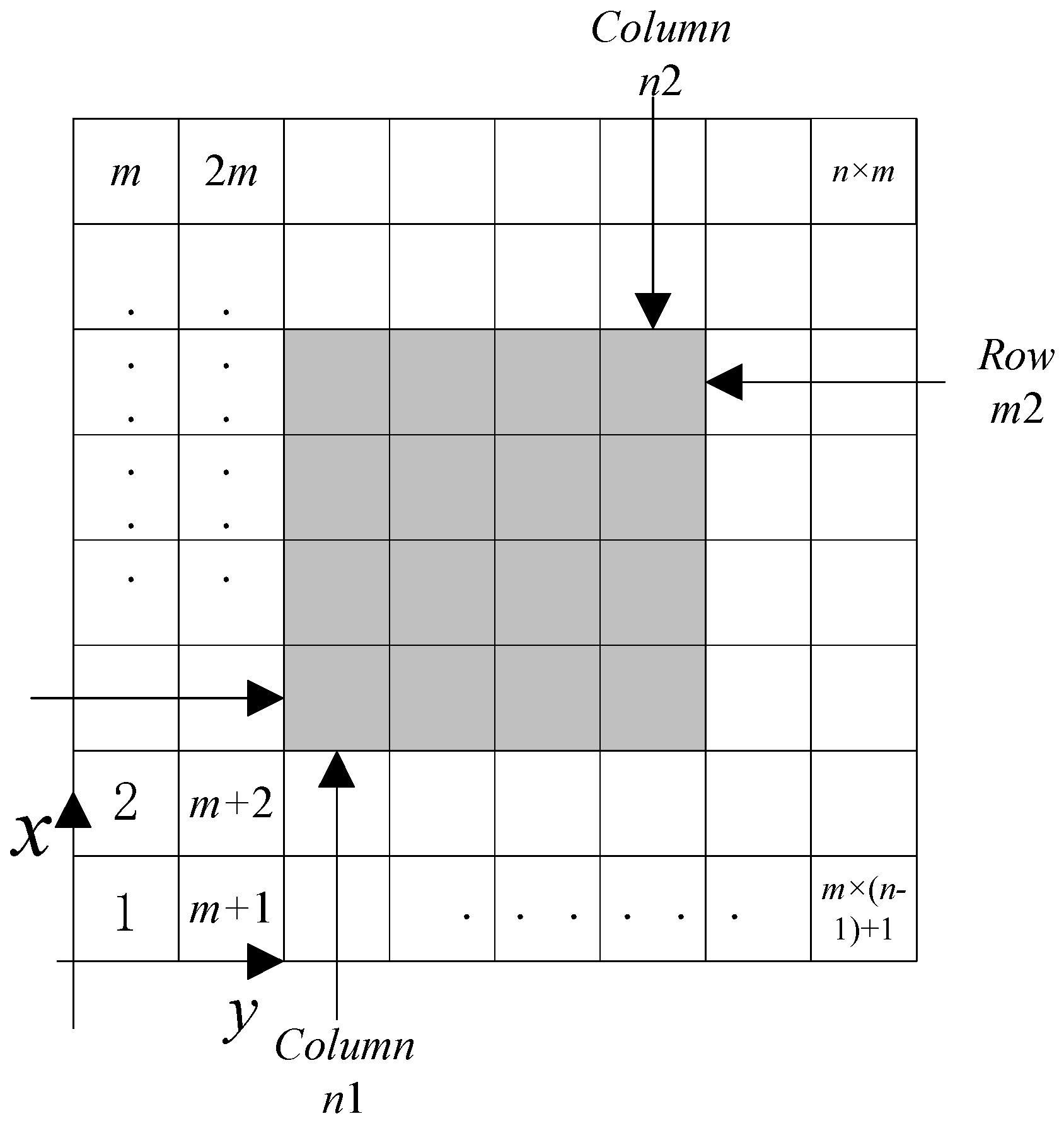
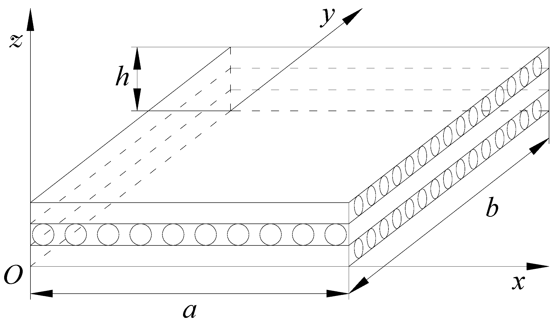
First, given a composite lamina size
a × b × h, we mesh the lamina board into the acquired size, whose quantity is
m × n × l, then locate the cubic damage edge on the lamina, supposing the damage area’s two vertex coordinates are (
x1,
y1,
z1) and (
x2,
y2,
z2), in which the damage area should be smaller than the lamina. Then, we can get this area’s element number in
Figure 1, and in the first layer we have the following:
The first layer damaged area element number is listed in
Table 1. In the
k-th layer, all the element node numbers should add the product of (
k − 1)
× m × n.Based on the damage size, the element numbers that need to be reduced or replaced within each layer are determined. Each element is assigned a material category code based on whether it needs to be reduced or replaced. For example, elements to be reduced are assigned the code “D”, while elements to be replaced are assigned the code “R”. Based on this, material properties are assigned to the elements by an encoded assembly function.
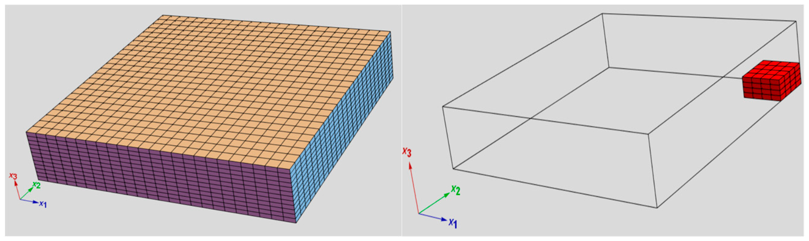
Figure 2 shows a quarter of a three-layered composite lamina; it was meshed into 24 × 24 in plane and 12 layers in thickness, and its damage area elements.
This method is very intuitive; the difficulty lies in coordinating the element partitioning with the damage size requirements. To ensure the calculation process does not result in a singular matrix, the stiffness of damaged elements is reduced by multiplying the healthy element stiffness by 1 × 10⁻¹¹.
3. Algorithm Validation and Its Application in Stress Analysis of Damaged Composite Materials
Example 1:
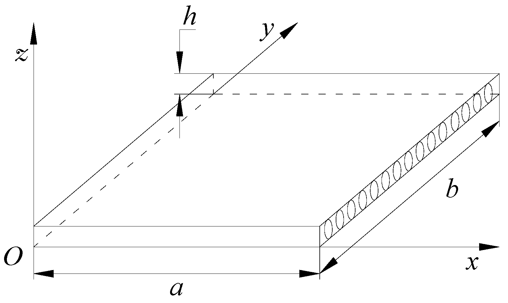
The first example is a single-layer-thick square plate, as shown in
Figure 3, with in-plane dimensions
a =
b, thickness
h, and the span-to-depth ratio
S =
a/
h = 10. The material properties are
Ex = 10,
Ey = 10
Ez,
Gxy =
Gxz = 0.6
Ez,
Gyz = 0.5
Ez, and
νxy =
νxz =
νyz = 0.25. The boundary conditions are
σxx = 0,
ux =
uz = 0 on
x = 0 and
x = a; and
σyy = 0,
ux =
uz = 0 on
y = 0 and
y =
b. The uniformly distributed load
q0 = 1.0 is on the upper surface of the plate. This particular problem has been investigated by Fan [
26].
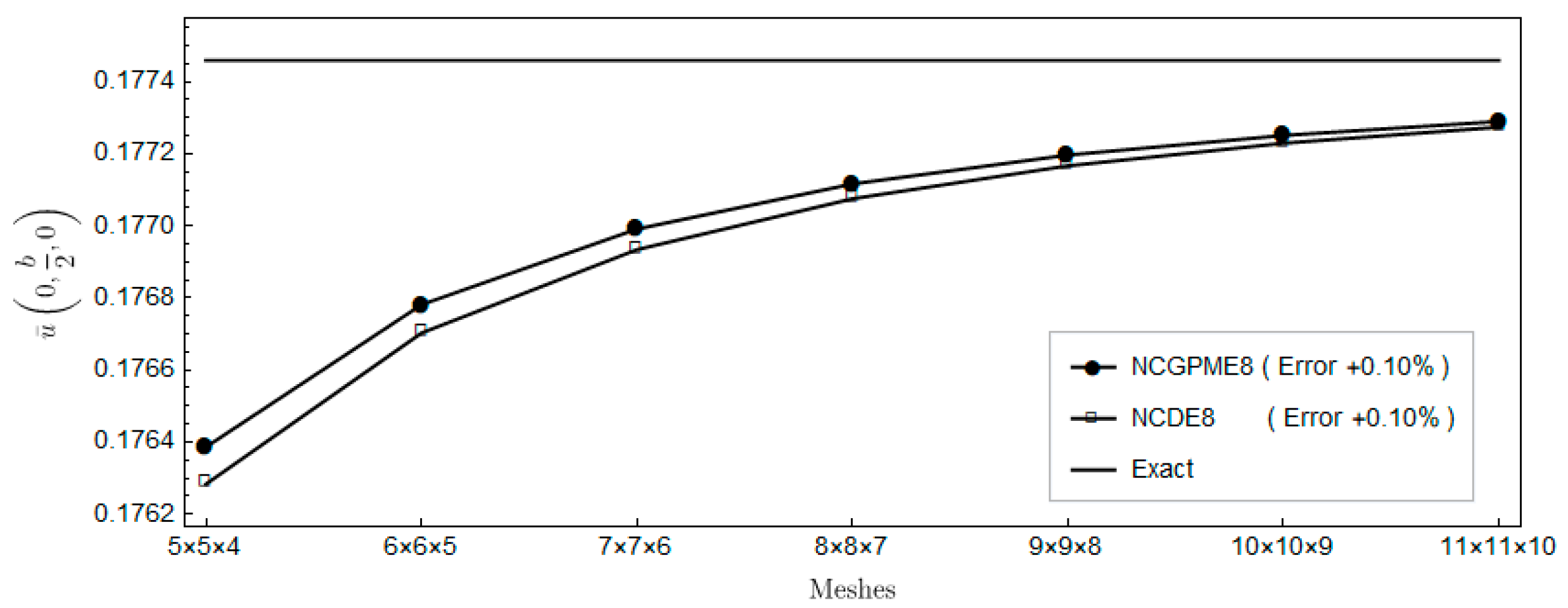
Due to the symmetry of the plate, only a quarter of the plate is analyzed. The notation l × m × n denotes l subdivisions along the x-axis and m subdivisions along the y-axis with the uniform elements; here n denotes the element number in the z direction. An amount of 2 × 2 × 2 Gaussian points and λ = 0.75 for each element are employed in our computer program.
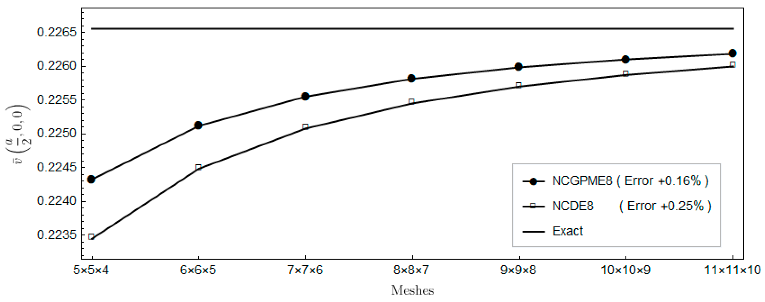
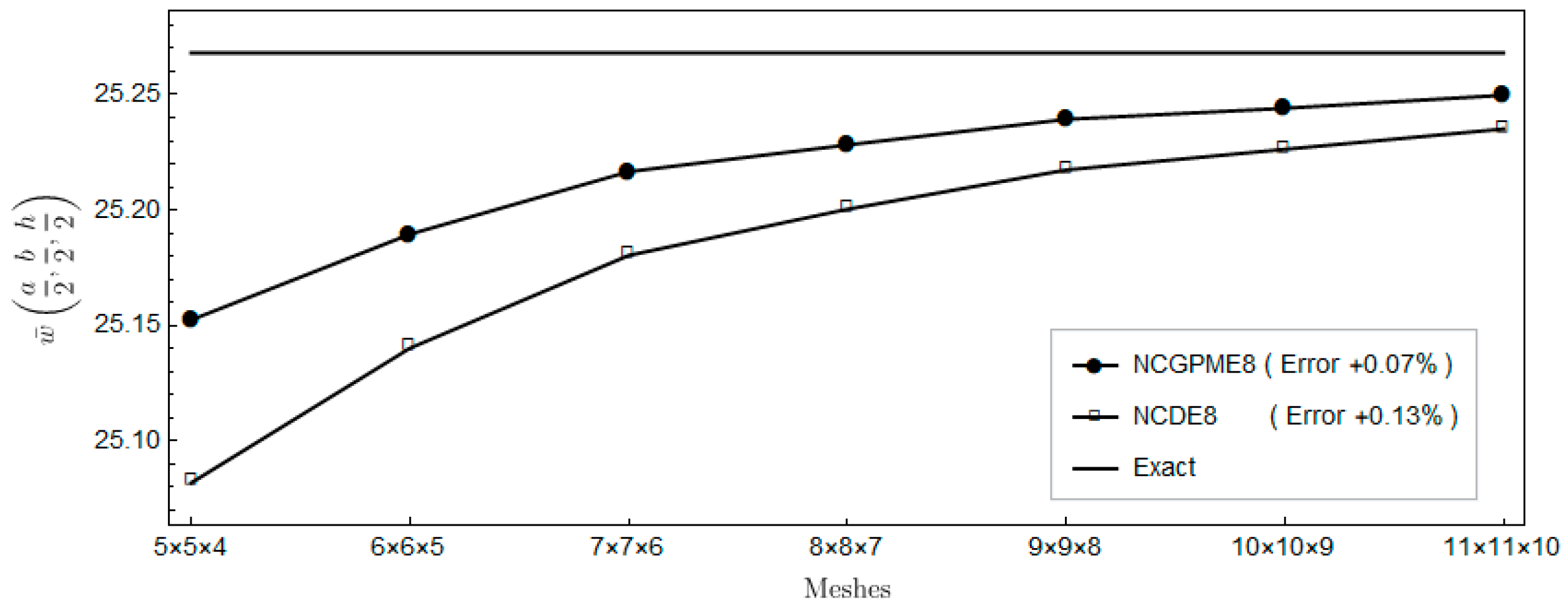
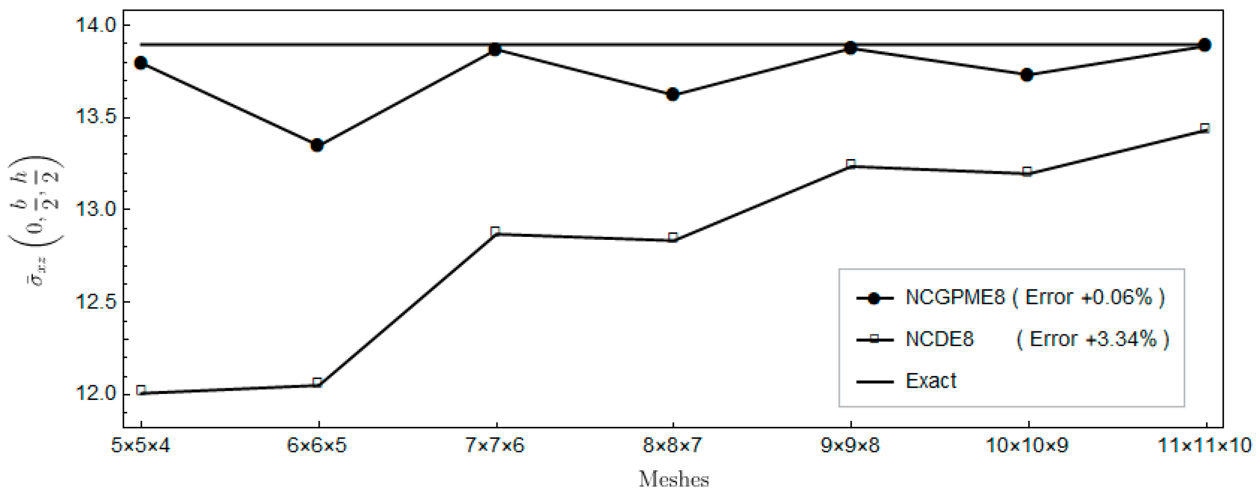
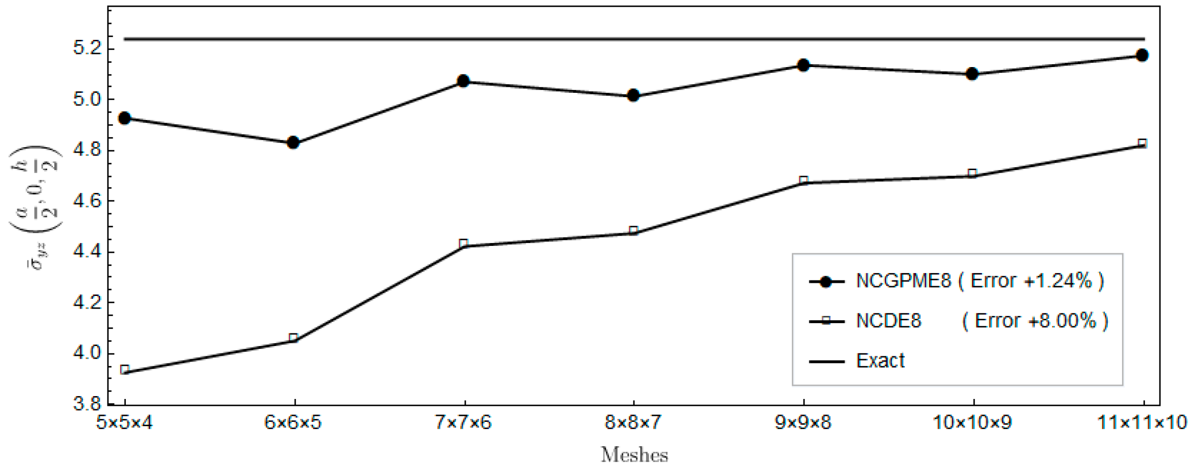
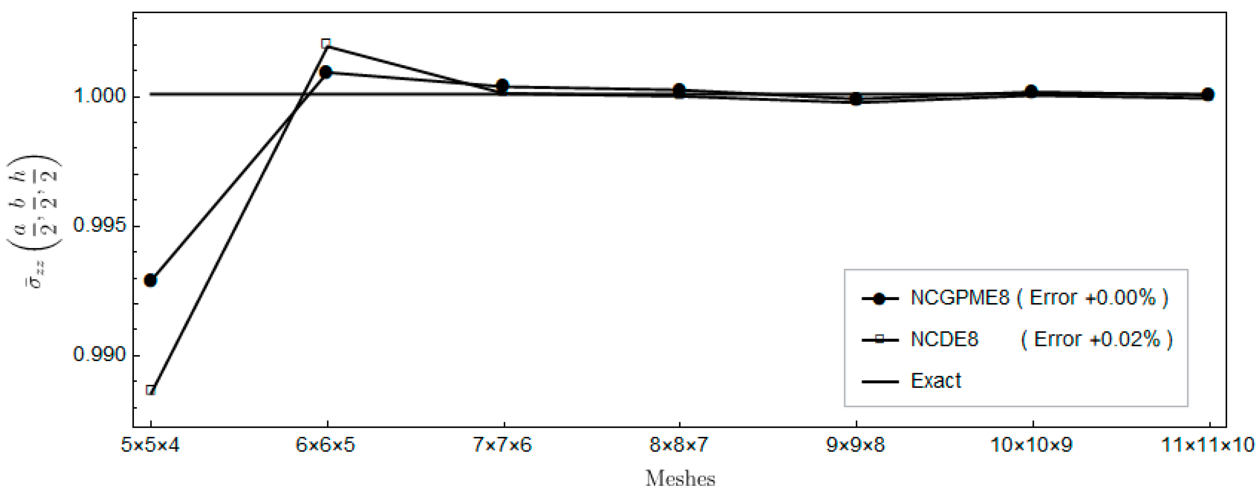
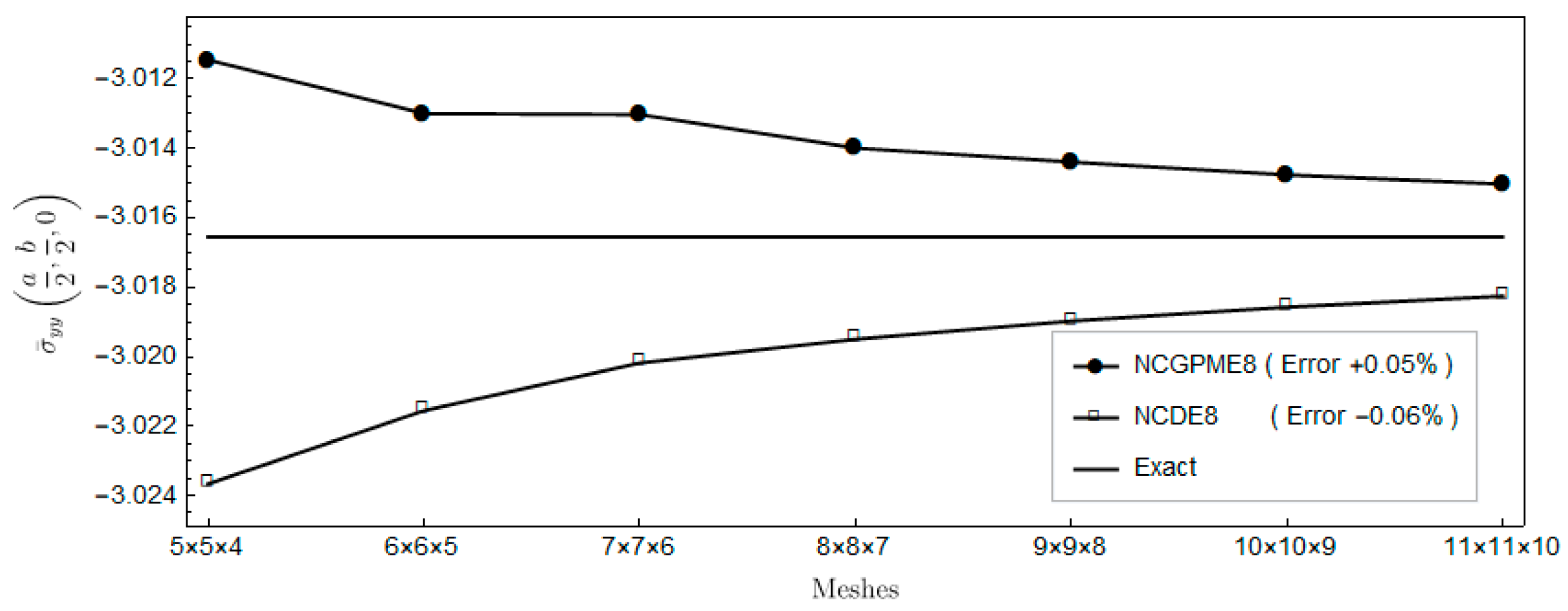
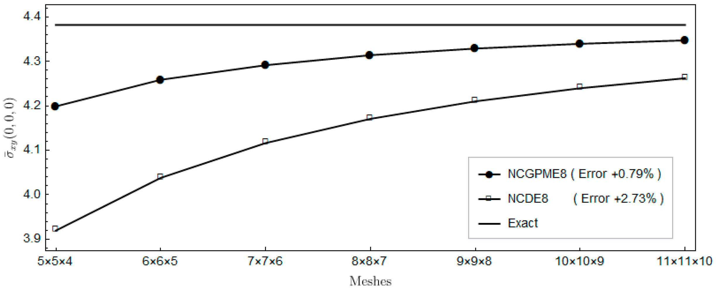
The nonconforming displacement element with eight nodes (NCDE8) in the commercially available software ABAQUS are obtained from the stresses of Gauss quadrature points by the extrapolation method [
10]. Based on the results of the 11 × 11 × 10 mesh, the percentage errors of displacements and stresses illustrated in the legends in
Figure 4,
Figure 5,
Figure 6,
Figure 7,
Figure 8,
Figure 9,
Figure 10,
Figure 11 and
Figure 12 are computed by (numerical-exact)/numerical, where “exact” denotes the exact solution and “numerical” is NCGPME8 or NCDE8. The exact solution is obtained by the method in reference [
26].
Figure 4,
Figure 5 and
Figure 6 show a comparison with the displacements obtained using NCDE8. The convergence of displacement of the present nonconforming generalized partially mixed element with eight nodes (NCGPME8) are slightly better than those of NCDE8.
Figure 7,
Figure 8,
Figure 9,
Figure 10,
Figure 11 and
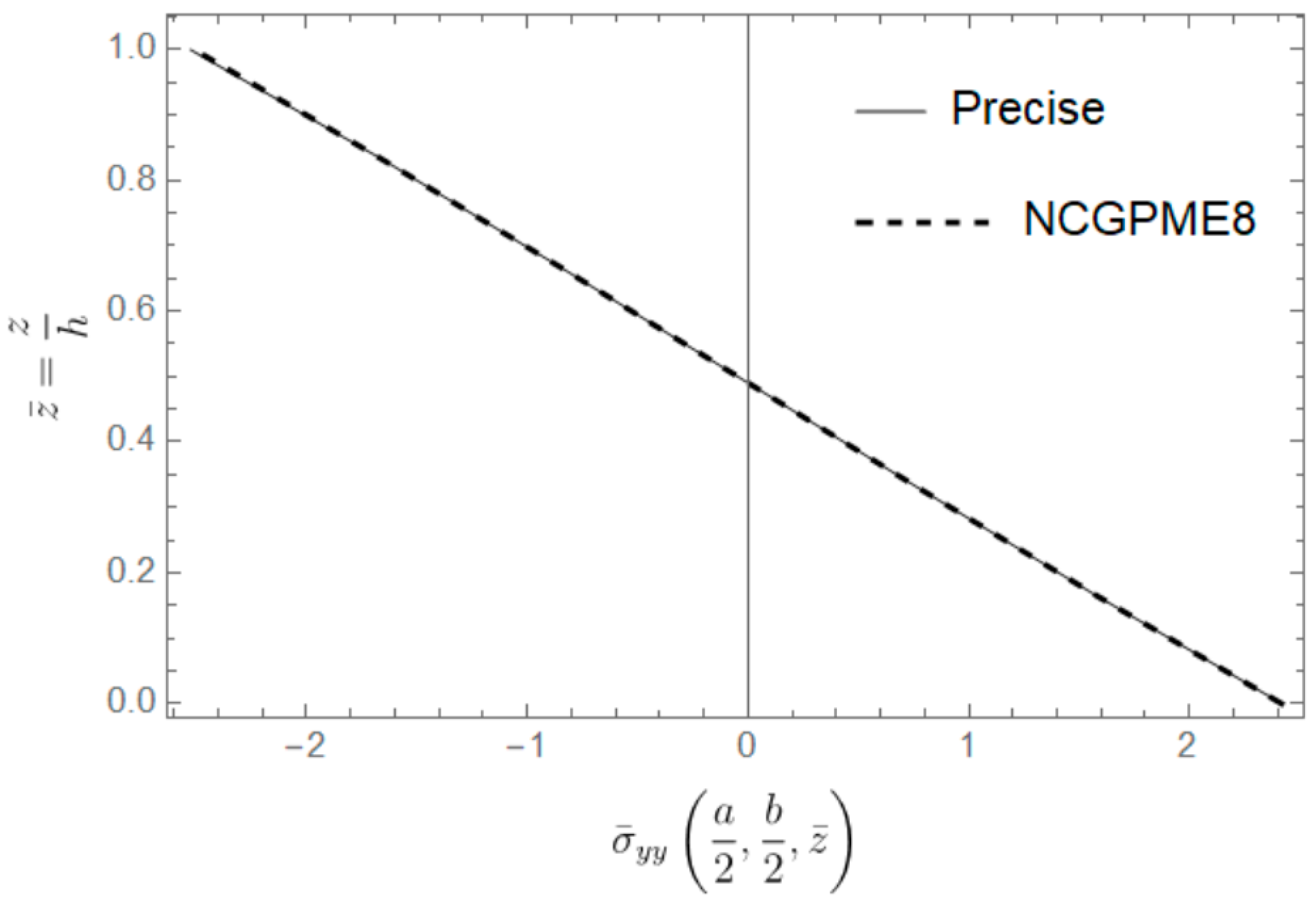
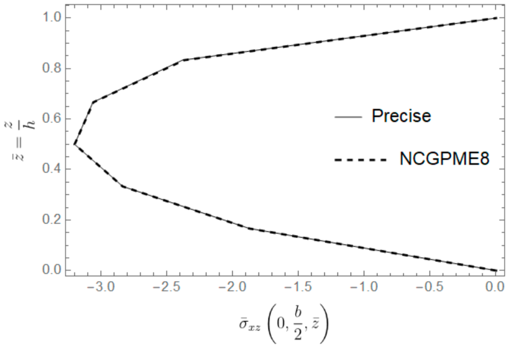
Figure 12 indicate that, for the same mesh, the out-plane stress results of NCGPME8 and the in-plane stress results of the finite element algebraic system are evidently superior to NCDE8. This superiority is more obvious for the two out-plane shear stresses, and the in-plane shear stress.
The foregoing comparison of NCDE8 and NCGPME8 seems unfair since, for the same mesh, the present mixed element has more degrees of freedom. However, it does highlight the advantage of having a continuous stress field with unique nodal values. Furthermore,
Figure 7,
Figure 8,
Figure 9,
Figure 10,
Figure 11 and
Figure 12 indicate that if one wants to get more accurate shear stress results, NCGPME8 does not require the extremely fine meshes that are needed by NCDE8.
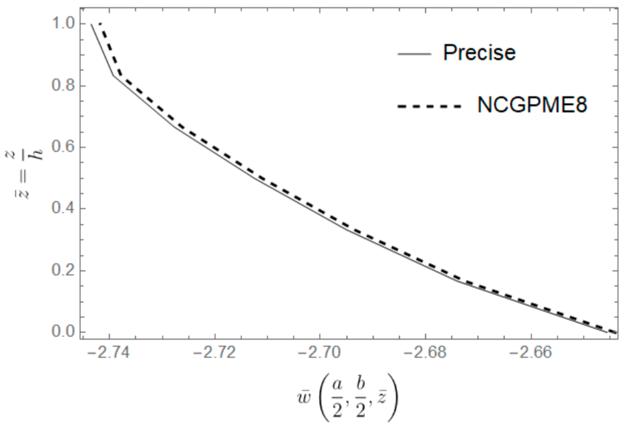
From
Figure 7 and
Figure 8, the two out-plane shear stresses of two elements oscillate with the increase in mesh density. The main reason is that, when the model is divided into an odd number of elements in the thickness direction, the results of the out-plane stresses
and
can be only obtained by interpolation based on the nodal stresses in the model. When the model is divided into an even number of elements in the thickness direction, the accuracy of the out-plane stresses
and
is relatively high since their values are on the nodes.
Example 2:
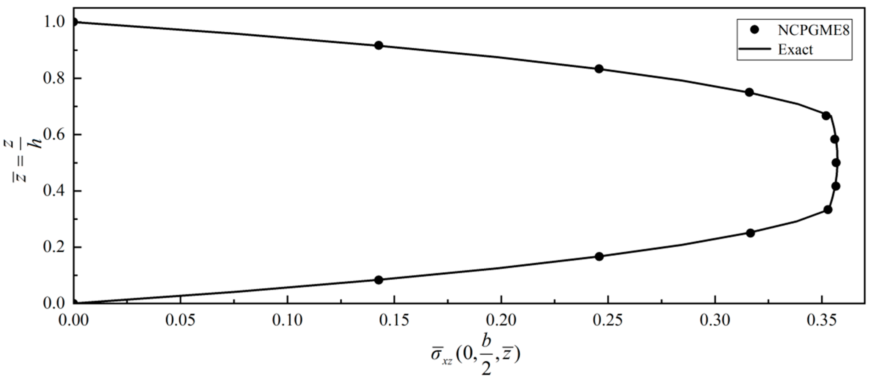
To demonstrate the accuracy of NCGPME8 in solving thick laminated plates, consider the following simply supported single-layer-thick plate with h/a = 0.2, where the length and width of the plate are a = b. The upper surface of the plate is subjected to a uniformly distributed pressure stress q = −1, with material properties that are the same as Example 1.
Define non-dimensional parameters as the following:
Organize
Table 2 and
Table 3 into a graph, which provides the following:
From
Figure 13,
Figure 14 and
Figure 15, it can be observed that the solution obtained by NCGPME8 for thick plates is very close to the exact solution, and it exhibits good convergence. The NCGPME8 element belongs to three-dimensional non-coordinated elements, taking into account the relationship between the plate deflection and the z-coordinate, and it can pass the Patch Test. The non-coordinated interpolation functions can describe irregular elements much better, and the partial mixed variable method can also ensure the stress continuity of individual nodes, thus ensuring the convergence and accuracy of the NCGPME8 method in solving small deformation problems for thick plates. In addition, the difference between the exact solution and the NCGPME8 solution is larger on the upper surface than on the lower surface, mainly because the deflection solution of the thick plate is influenced by the z-coordinate.
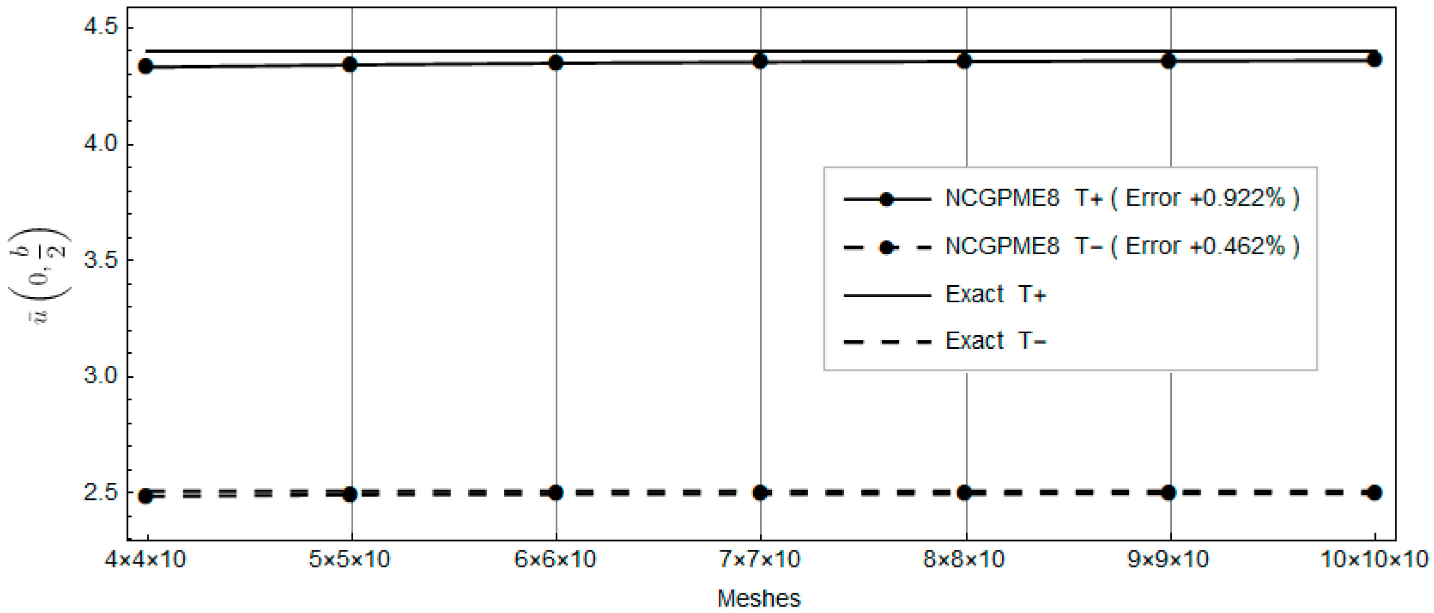
Example 3:
In order to demonstrate the convergence of NCGPME8 under the assumption of small deformation in a linear elastic body, numerical calculations were conducted for a four-edge simply supported honeycomb square plate. The boundary conditions are simply supported, the same as Example 1. The plate has upper and lower surface layers, as well as a honeycomb core layer. The material parameters are specified as follows:
According to Fan [
26], the dimensionless parameters are defined as follows:
The material parameter ratio between the surface layers and the honeycomb core is denoted by
, where
represents the material parameter of the surface layers, and
represents the material parameters of the honeycomb core. The total thickness of the plate is denoted as
, with the upper and lower panel thicknesses both equal to
, and the honeycomb core thickness is 0.8
h. The upper surface is subjected to a uniform distributed pressure
, while the lower surface is free. Fan Jiarang [
26] solved this problem and the results are shown in
Table 4.
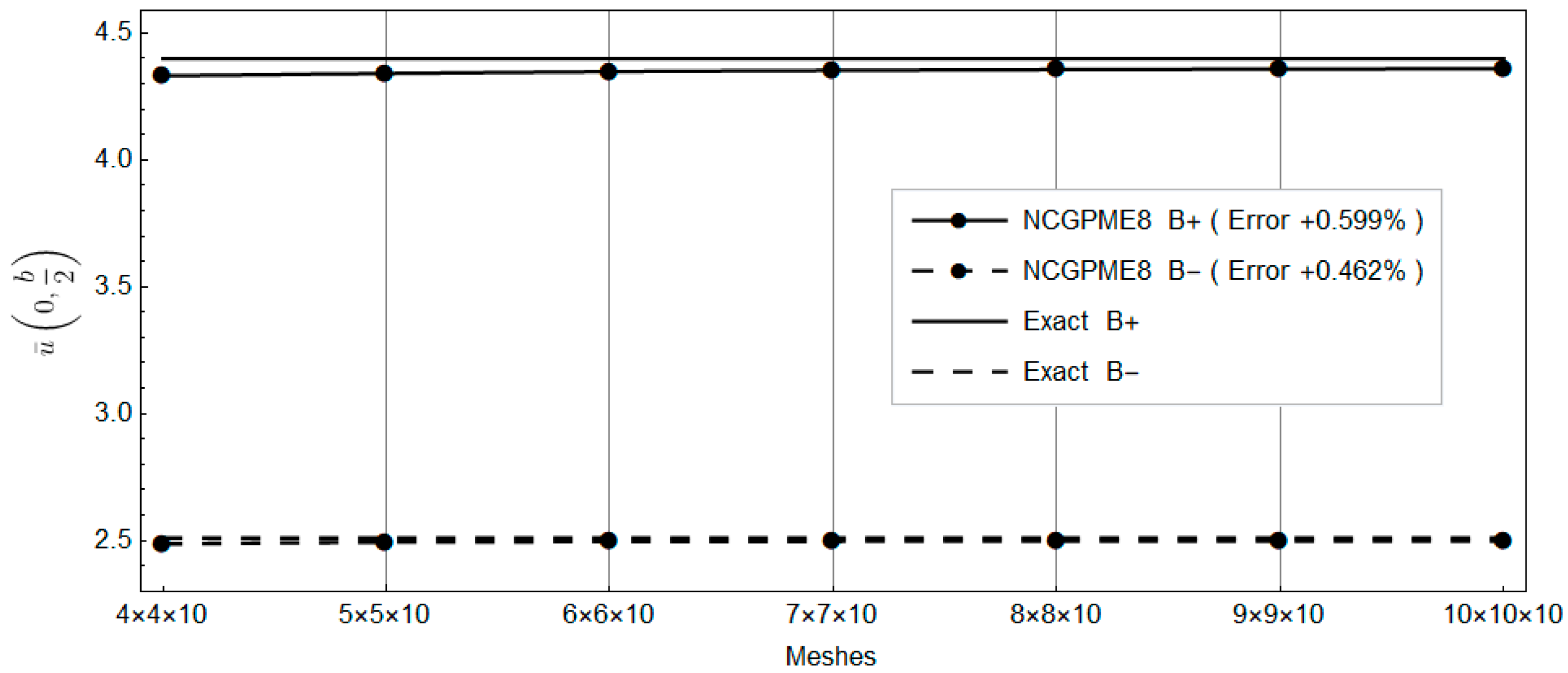
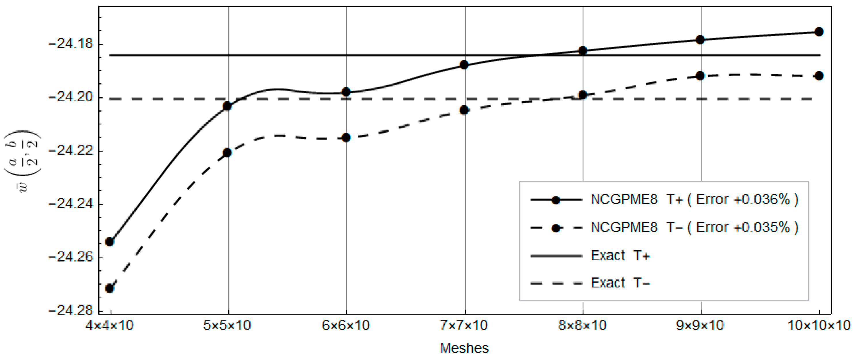
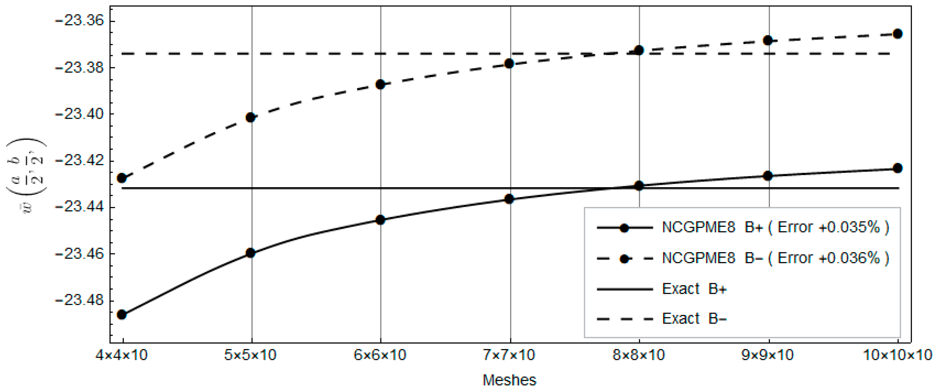
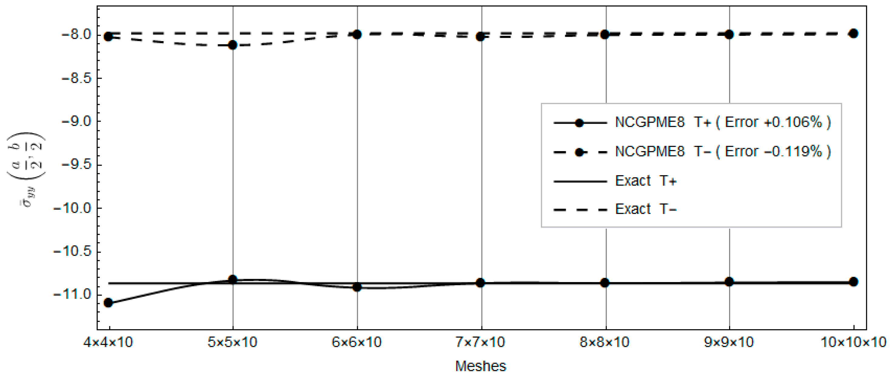
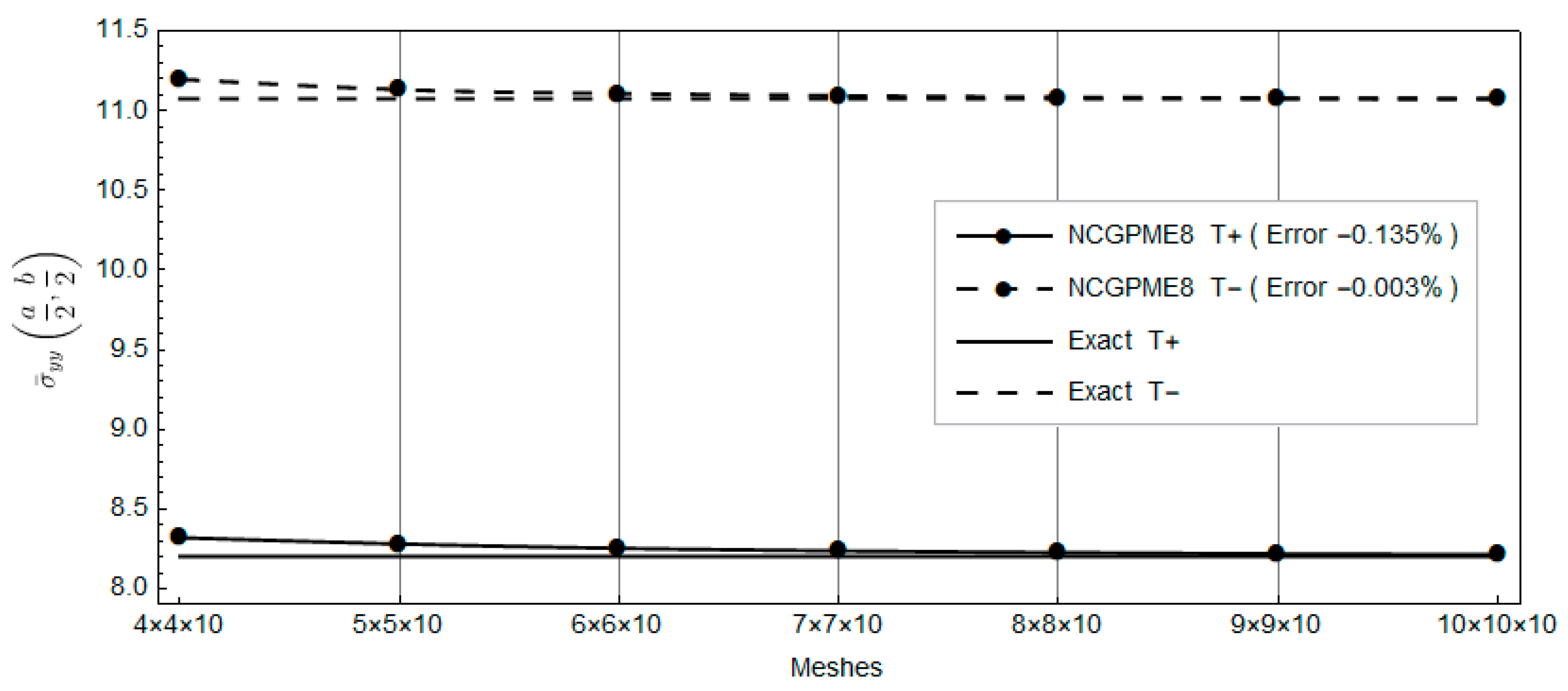
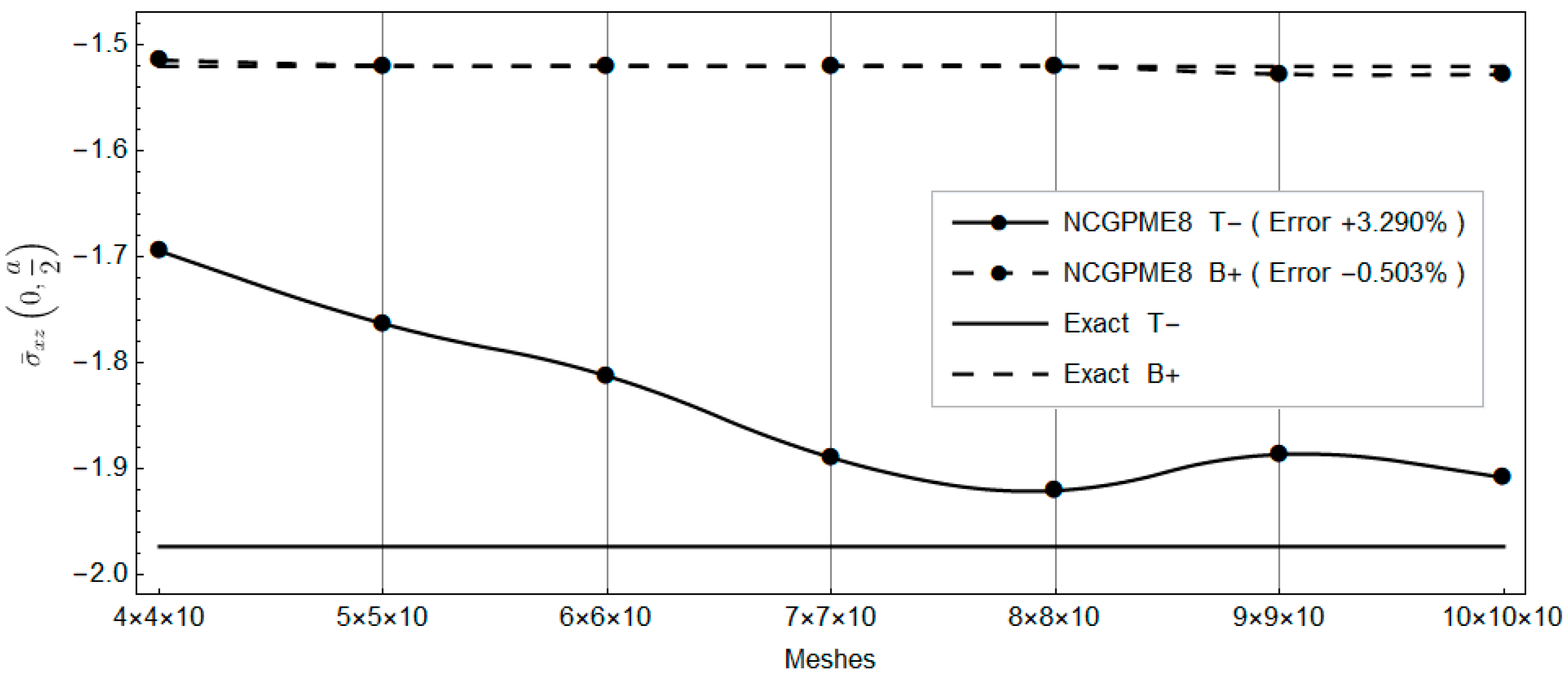
Due to the symmetry of the plate, an analysis using the NCGPME8 element () was performed on a quarter model. In the thickness direction, each of the upper and lower panels consists of one layer, and the middle honeycomb core is divided into eight uniformly distributed layers, resulting in a total of 10 layers.
In
Table 4, T represents the top layer and B represents the bottom layer, where + and − indicate the top and bottom surfaces of a layer, respectively.
Clearly, with the increase in planar mesh, the rapid convergence of NCGPME8 can be observed in
Figure 16,
Figure 17,
Figure 18,
Figure 19,
Figure 20,
Figure 21 and
Figure 22. It is noteworthy that the error in the solution for in-plane stresses is small, as evident from
Figure 20 and
Figure 21. Although the
values for the upper and lower panels exceed the exact solution of Fan [
26], the solution from this method becomes noticeably convergent with mesh refinement. In
Figure 22, the error in the upper panel’s out-of-plane stress
is within 3%, which is acceptable. This example verifies the correctness of the stress analysis method for laminated plates based on the eight-node non-conforming generalized partially mixed element and the accuracy of the algorithm in calculating in-plane stresses.
Example 4:
As shown in
Figure 23, the non-dimensionalized size of the laminated plate is
a =
b = 10
h, with each layer having an equal thickness and a ply orientation of [0°/90°/0°]. The boundary conditions are the same as Example 1. Each layer of the laminated plate is idealized as a homogeneous orthotropic material. The material properties of the laminated plate in the main material direction are the following:
Exx = 25.0,
Eyy = 1.0,
Gxy = 0.5,
Gxz = 0.2,
νxy =
νxz = 0.25.
A normal out-of-plane load
q(
x,
y) =
q0 Sin(
πx/
a)
Sin(
πy/
b) is applied to the top surface, where
q0 = 1, and the bottom surface is free. Pagano [
27] studied laminated plates adopting the elasticity theory.
In this example, due to symmetry, only a quarter of the plate is discretized. A uniform grid of 12 × 12 × 12 is used to calculate the stress distribution along the thickness direction.
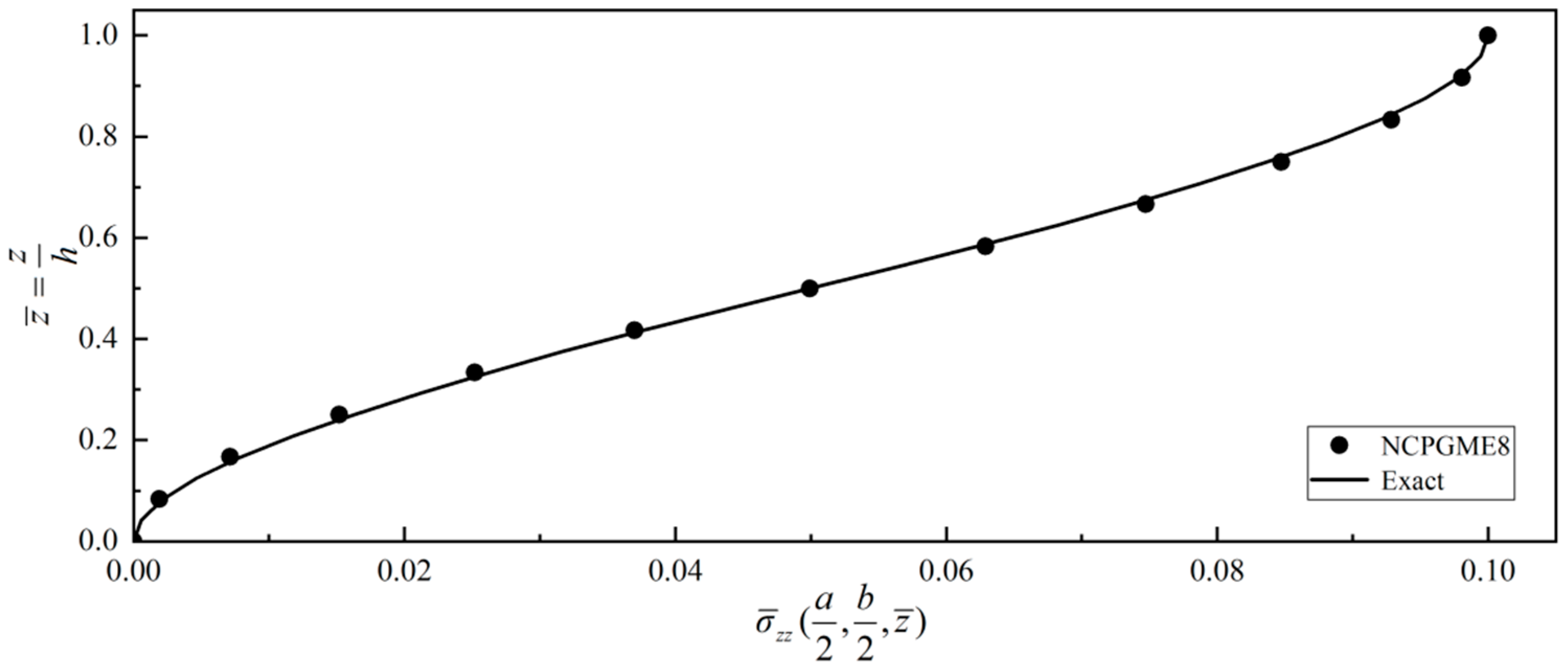
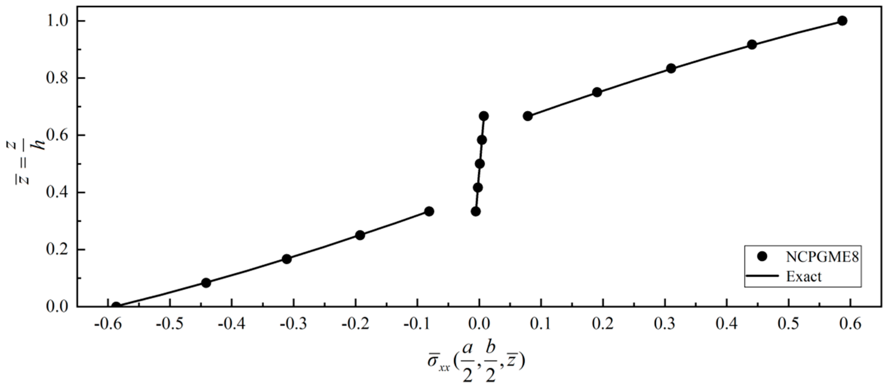
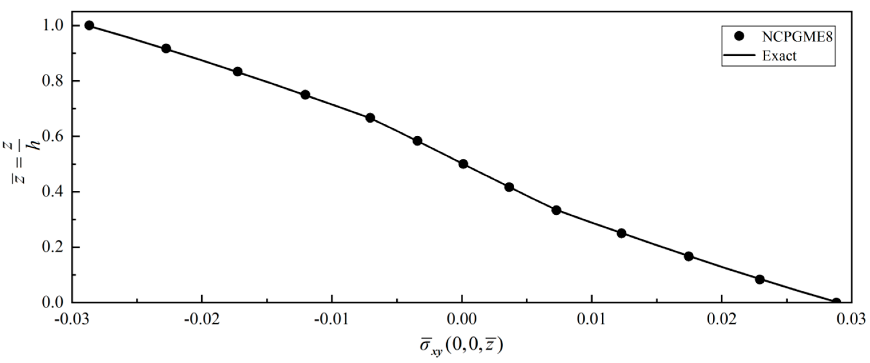
Figure 24,
Figure 25,
Figure 26 and
Figure 27 show four typical stress distributions obtained by NCGPME8 (λ = 0.75) as given by Equations (34) and (35).
It should be noted that in this example, all parameters are normalized, and the expressions are the same as Example 1:
Figure 24,
Figure 25,
Figure 26 and
Figure 27 show that the stress distribution along the thickness direction matches well with the exact solution. When a 12 × 12 × 12 discrete grid is used, the error in the stress distribution along the thickness direction is less than 0.5%.
As the out-plane shear stress boundary conditions on the plate surface can be fulfilled in some mixed models, the outcomes of the out-plane shear stress on the upper and lower surfaces are fit to the given boundary conditions, as shown in
Figure 24 and
Figure 25.
Besides,
Figure 26 shows the discontinuity of the interlaminar in-plane stress.
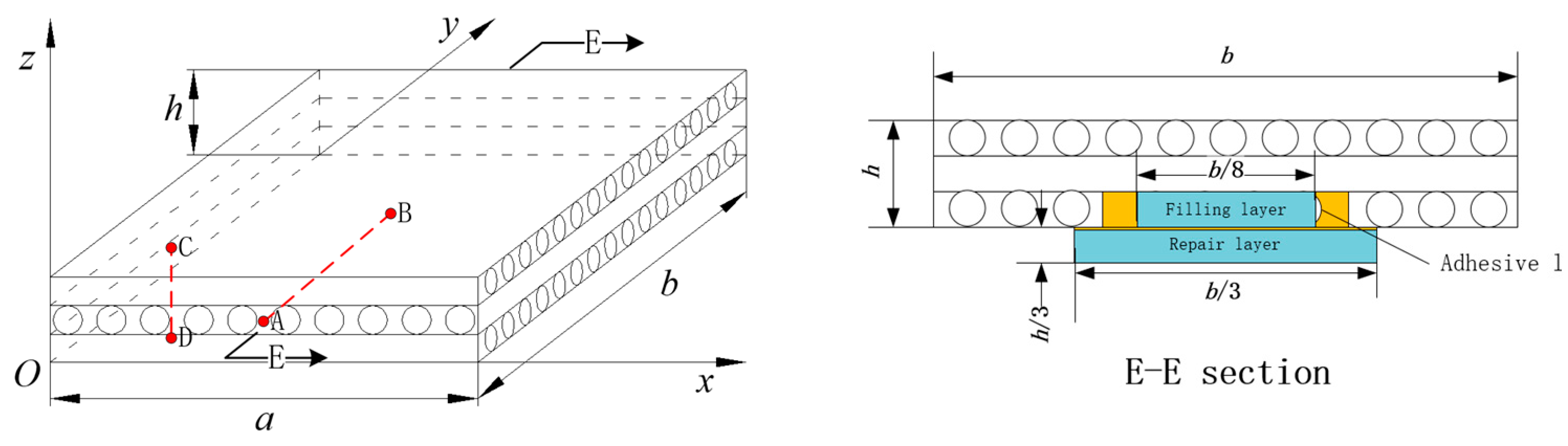
Example 5:
Given that the forgoing examples have demonstrated the convergence and accuracy of NCGPME8 and its ability to accurately solve internal stresses, this method is employed to analyze and compare composite materials, including healthy plates, damaged plates, and layered plates after step scarf repair. The models, boundary conditions, and loading methods used in this example are the same as in Example 4. Referring to Shen [
30], the elastic modulus of the isotropic adhesive layer E= 1.077 GPa, shear modulus G = 0.40489 GPa, and Poisson’s ratio μ= 0.33. A 48 × 48 grid is used to divide the plate in the
oxy plane, and the z-direction finite element model is divided into 12 layers for healthy and damaged plates, while the repaired plate was divided into 16 layers for a patch and was attached to the surface. The normalization method for parameters in this example is the same as in Equation (38).
For the damaged model, assume there is a damage in the center of the upper surface of the plate with dimension
, and the damage extends to a depth of
. The damaged material stiffness coefficient is derived by multiplying the healthy element stiffness by 1 × 10
−11. According to Equations (31) and (32), we have
The damaged elements number is listed in
Table 5.
The stiffness of the damaged element is approximated by multiplying the material parameters of the healthy plate by a factor .
For the repaired plate model, after removing the damage, a filling layer with dimensions
is first placed at the damaged location, and then an outer repair layer with dimensions
is attached, and the gap is filled with adhesive. The material parameters of the filling layer and the repair layer are the same as the original layer of the repaired item. The E–E cross-sectional view in
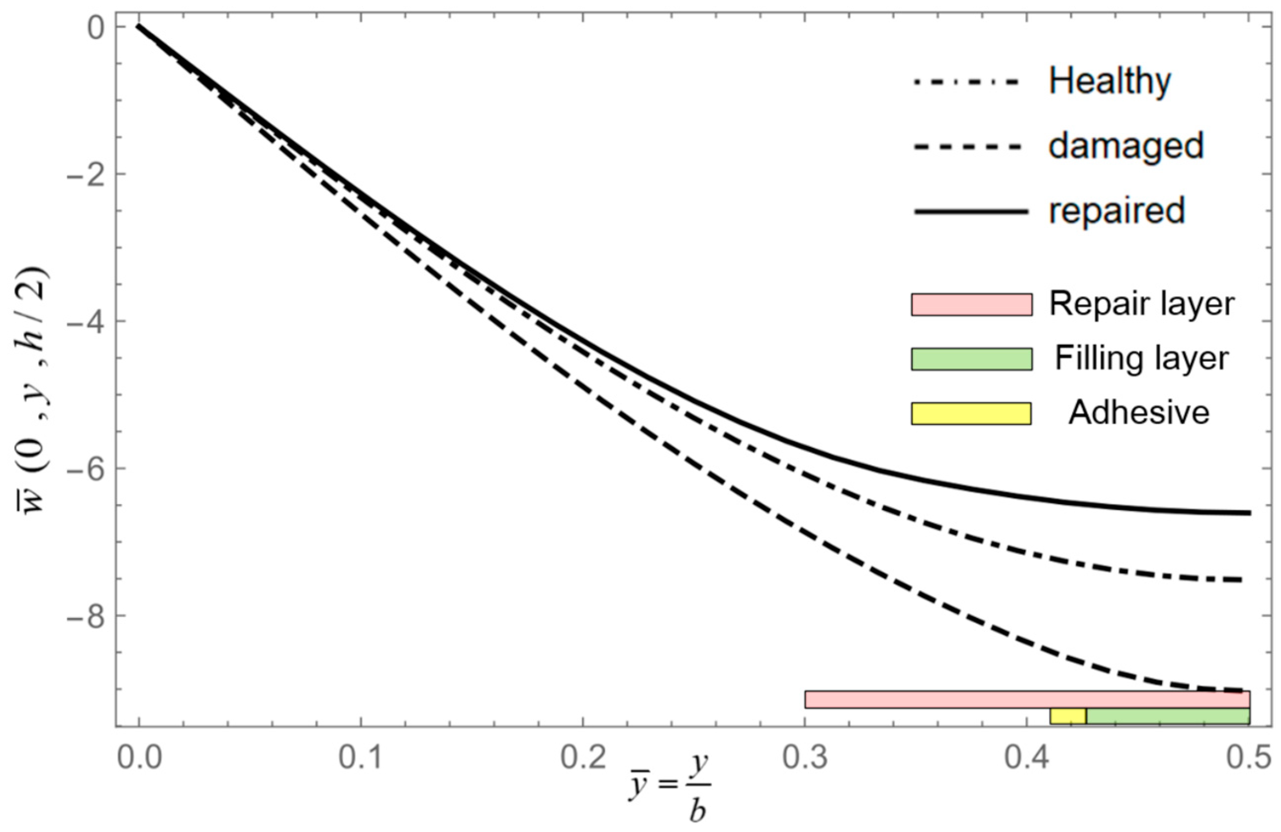
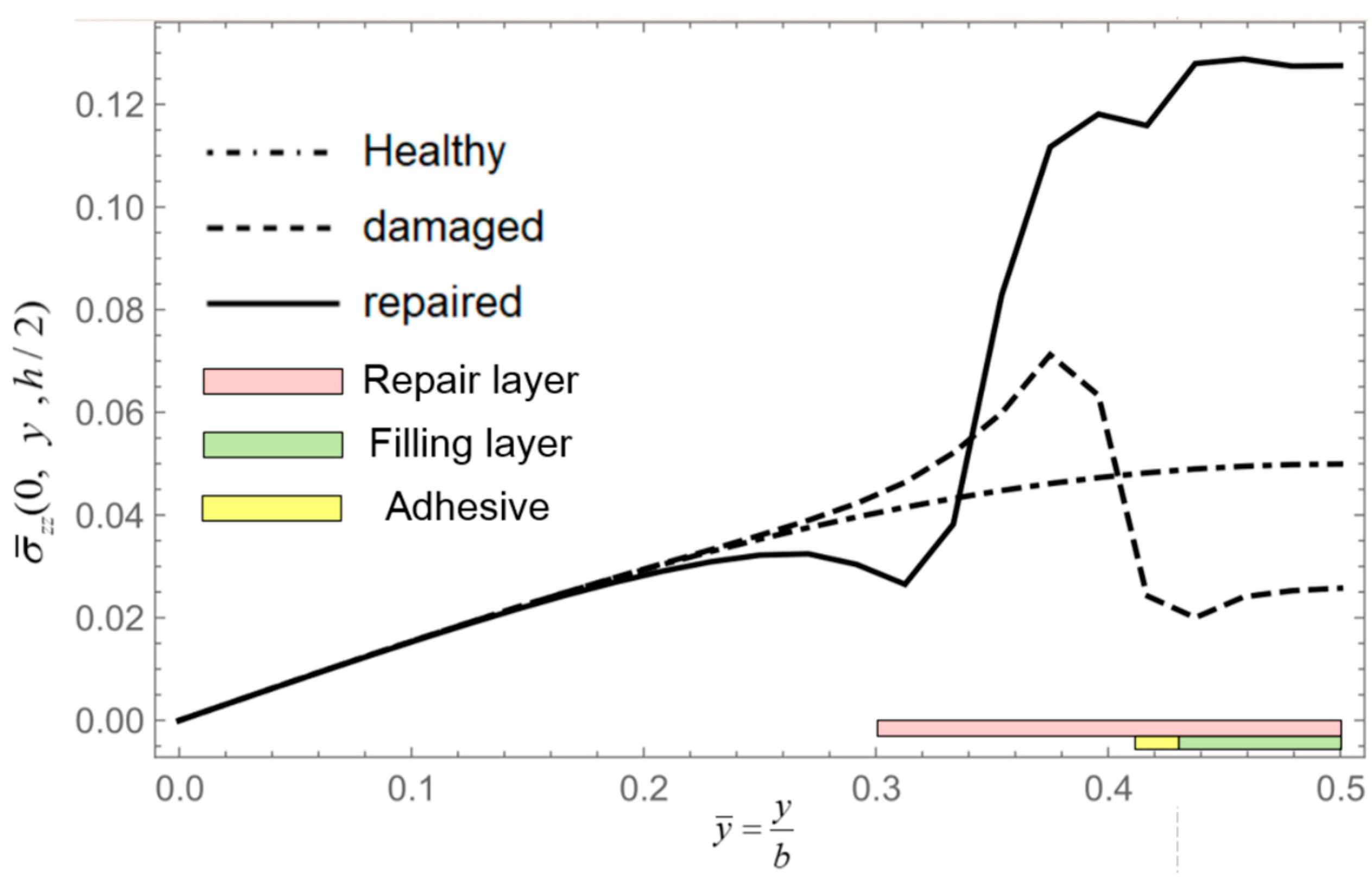
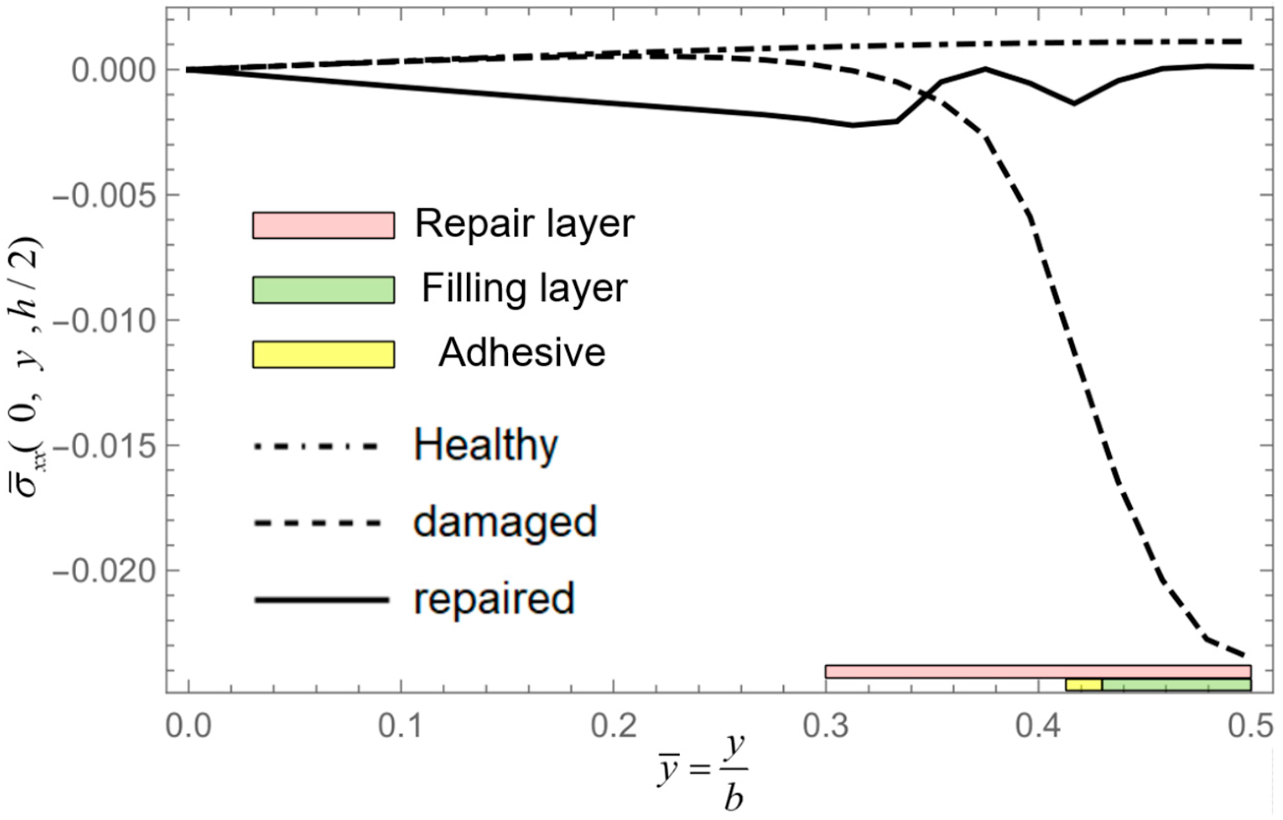
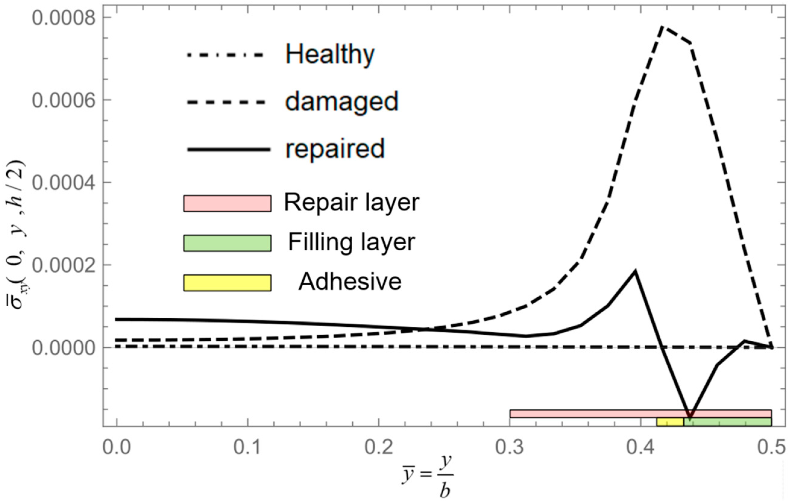
Figure 28 illustrates this configuration.
To the different health conditions of the plates, we compared their displacement
and stresses
,
,
along the line connecting
and
in
Figure 28. We also compared the in-plane stresses
,
,
along the line connecting
and
.
According to
Figure 29 and
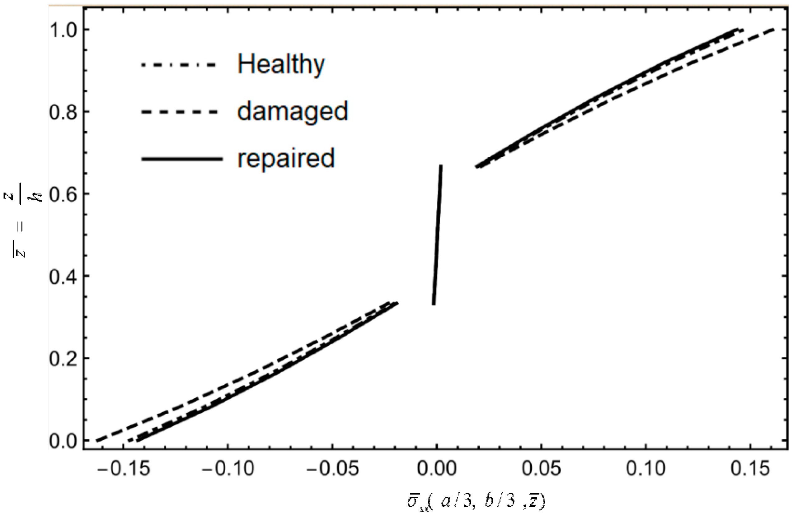
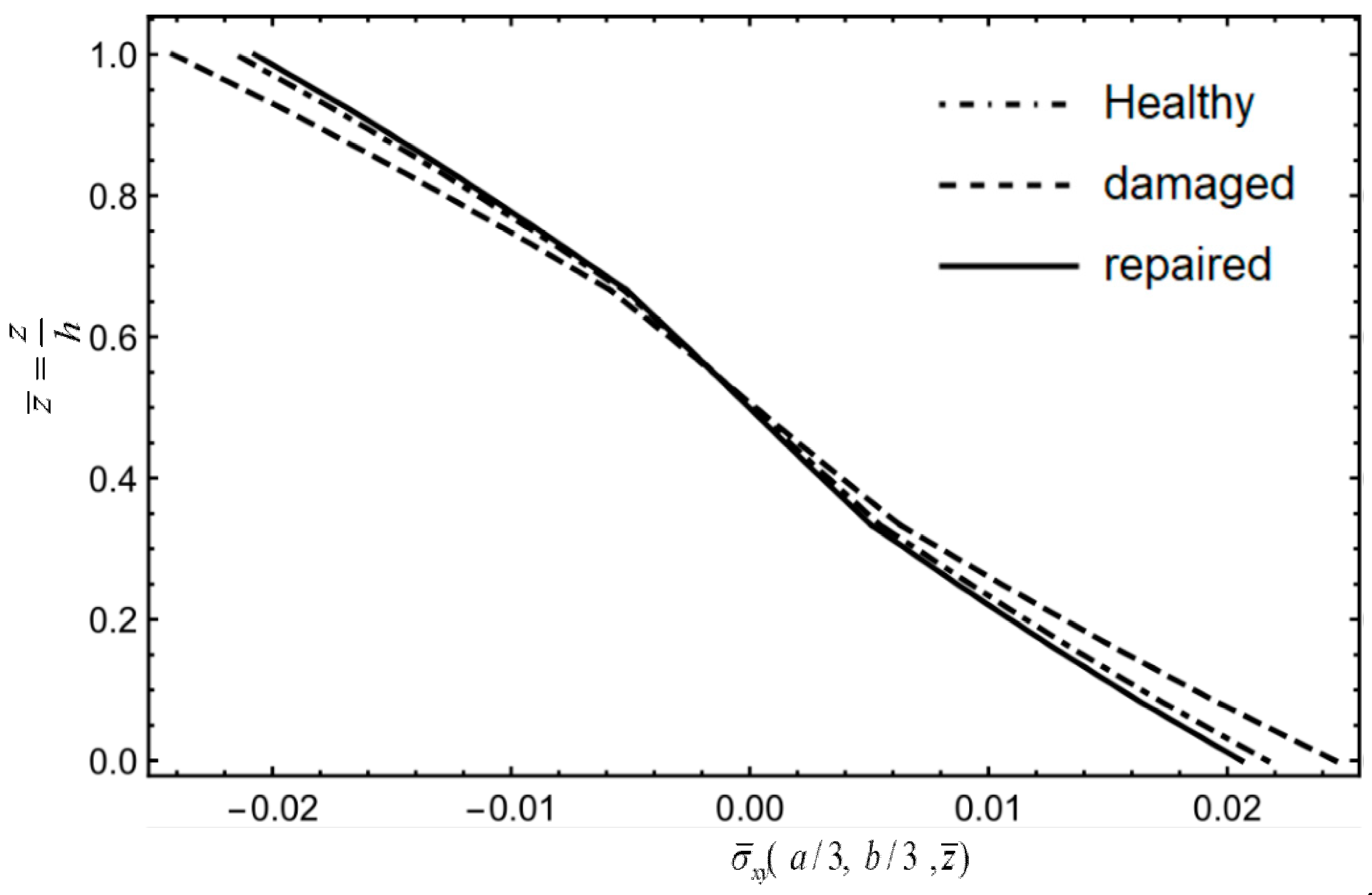
Figure 30, we know that damage reduces the local stiffness of the laminated panel, while repair enhances the local stiffness of the laminated panel. Correspondingly, the out-of-plane stresses are affected by damage and repair patches, leading to fluctuation across AB. From
Figure 31 and
Figure 32, we acquire that the in-plane stresses
,
of the damaged panel significantly increased; this is mainly due to the reduction in stiffness of the surface layer in the damaged panel, resulting in higher in-plane stresses borne by the intermediate and bottom layers. Due to the presence of adhesive layers between the panel and the filling layer, as well as the reinforcing effect of the repair patch, in-plane stresses
also exhibit fluctuations along AB as shown in
Figure 32.
Figure 33 and
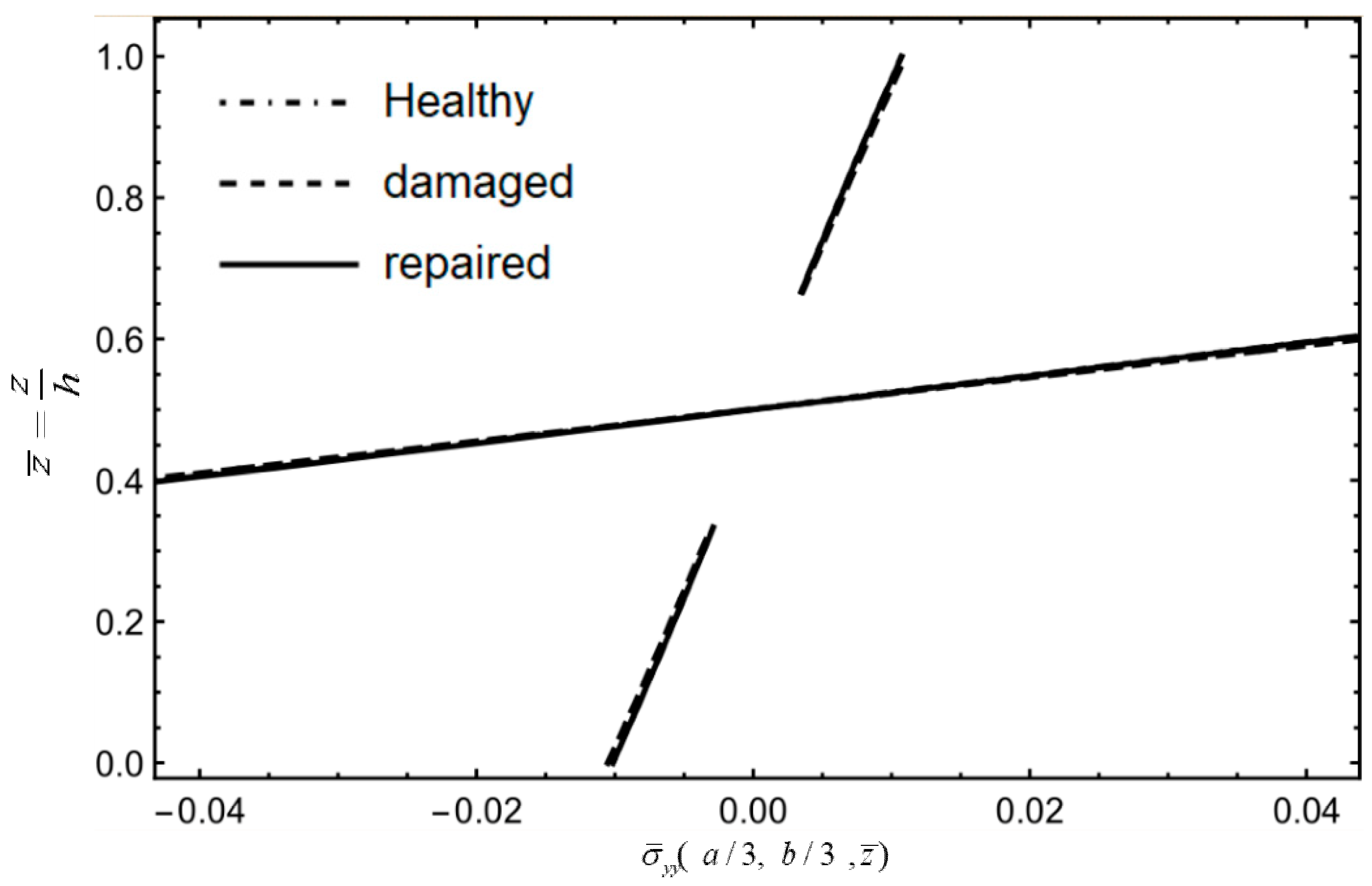
Figure 34 indicate that under fixed boundaries and loading conditions, the stress variation of
,
in the middle ply remains small for all three conditions, while the stresses at the top and bottom plies of the damaged part
,
show significant changes. This results in an increase in in-plane stress, making it more prone to interlaminar shear failure. In
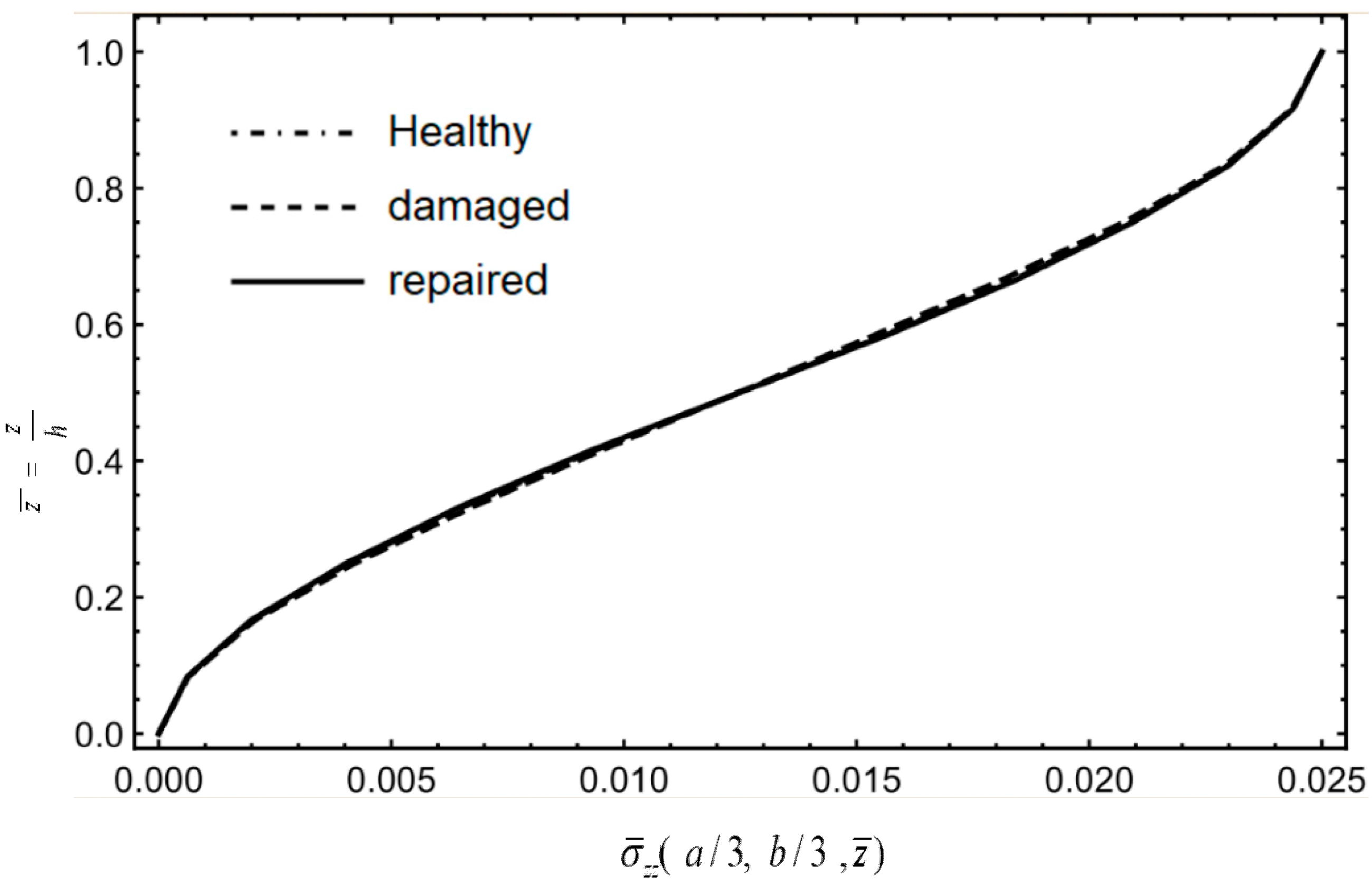
Figure 35, stress
is mainly carried by the matrix material of the middle plies and the fibers of the middle 90° ply. After damage to the top ply, stress
increases slightly in the top and bottom surface plies. After repair, stress
closely aligns with the healthy board, indicating minimal influence from damage or repair.
Figure 36 demonstrates that stress
has a distribution that is similar between the healthy board and the repaired board, with only a slightly increased slope for the damaged board, suggesting that damage results in more pronounced stress changes and a higher susceptibility to delamination or debonding.


