
An Event-Driven Link-Level Simulator for the Validation of AFDX and Ethernet Avionics Networks
 , ,
, ,  , , ,
, , ,
Abstract
:1. Introduction
2. Avionic Protocols
2.1. ARINC 664
2.2. Time-Sensitive Networking
3. Proposed System
3.1. General Framework
- Delay. Includes the maximum, minimum, mean, and standard deviation values of each flow/VL in milliseconds. The delay is set as the time from departure to arrival.
- Jitter. Includes the maximum, minimum, mean, and standard deviation values of each flow/VL in milliseconds.
- Throughput. Includes the maximum, minimum, mean, and standard deviation values of each flow/VL in bits per second (bps).
- Packet loss. Specified for each flow/VL as a percentage.
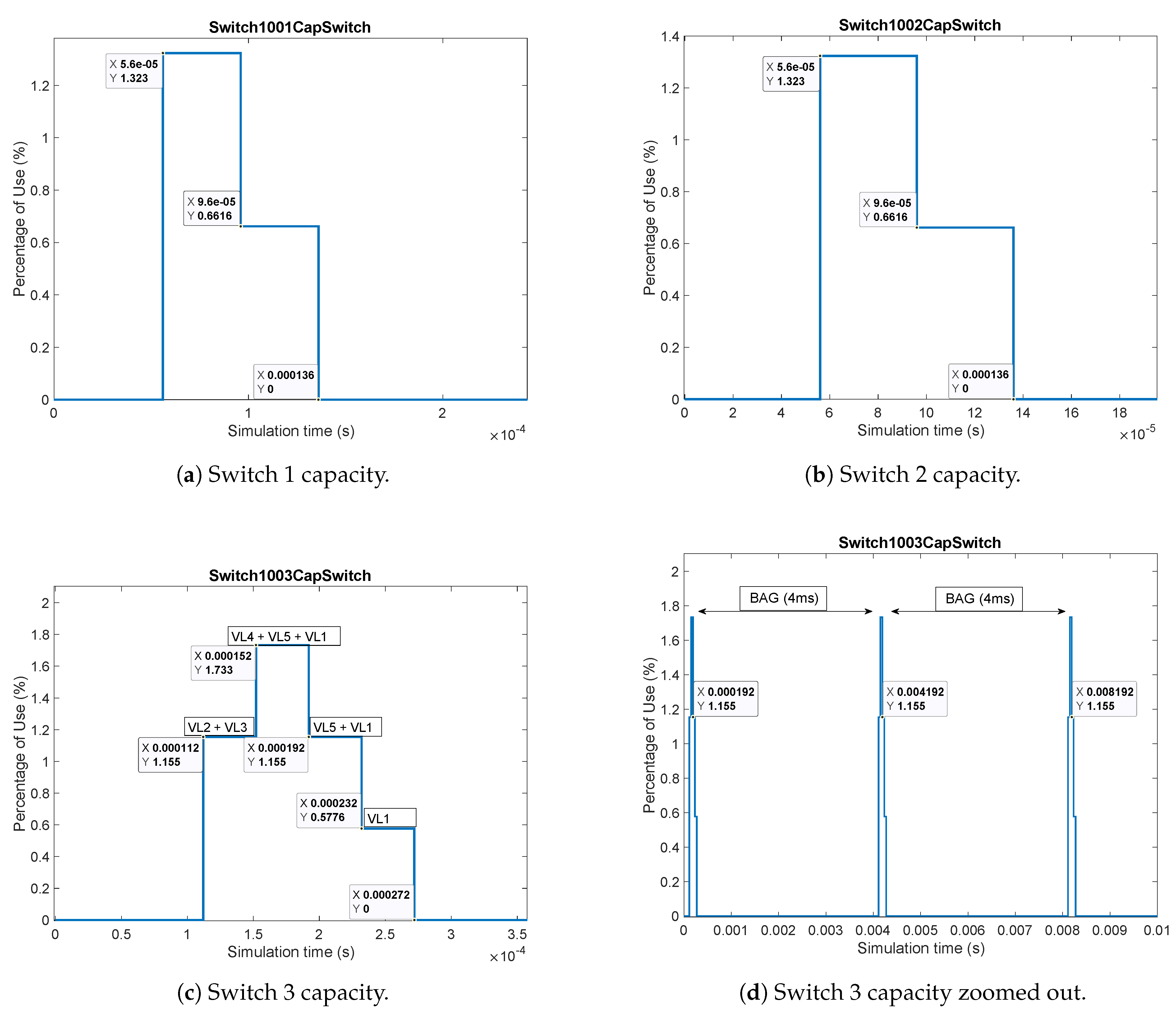
- Switch capacity. General capacity of each switch through the simulation in percentage.
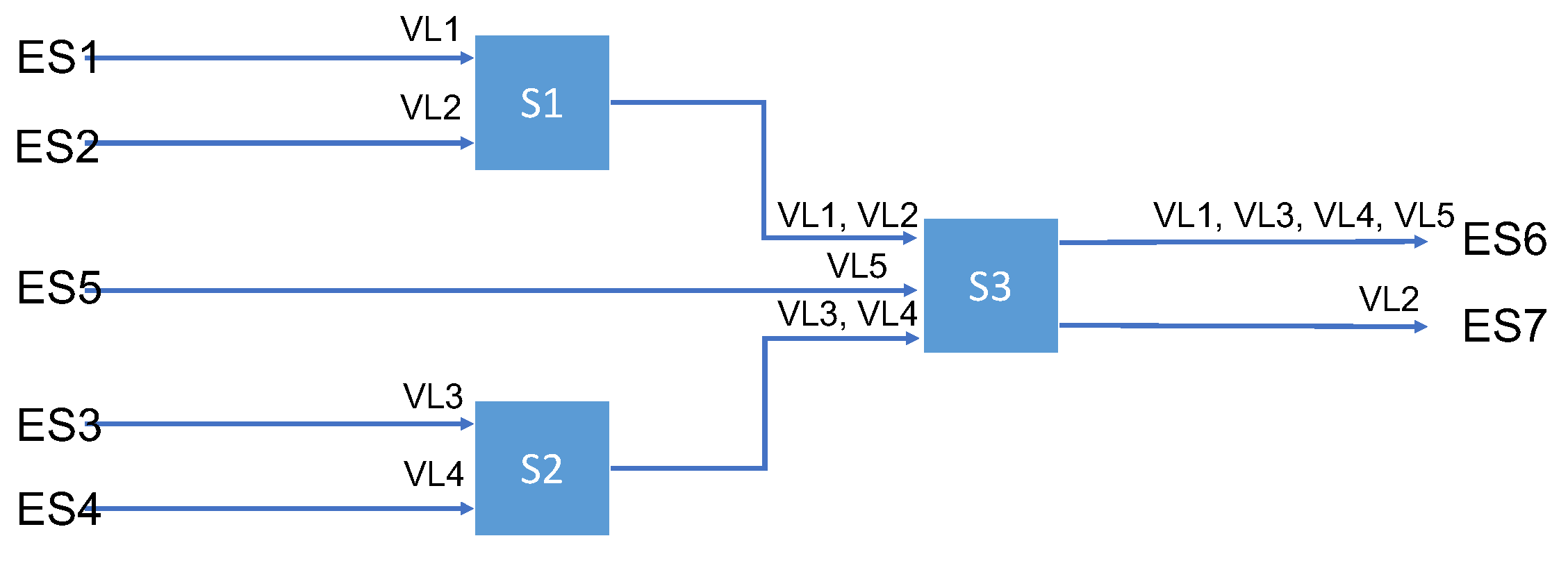
3.2. Multiple VL/Path Configuration
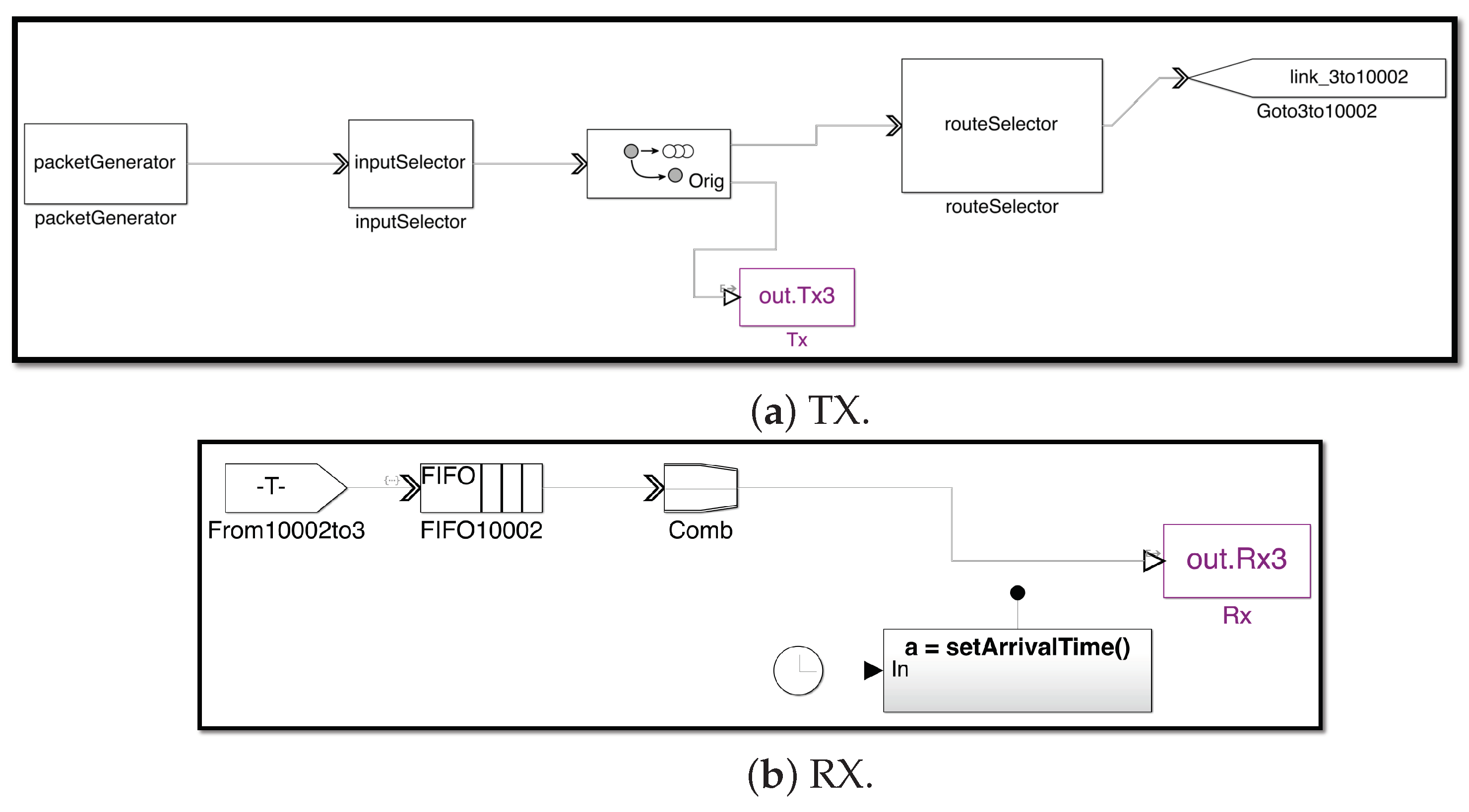
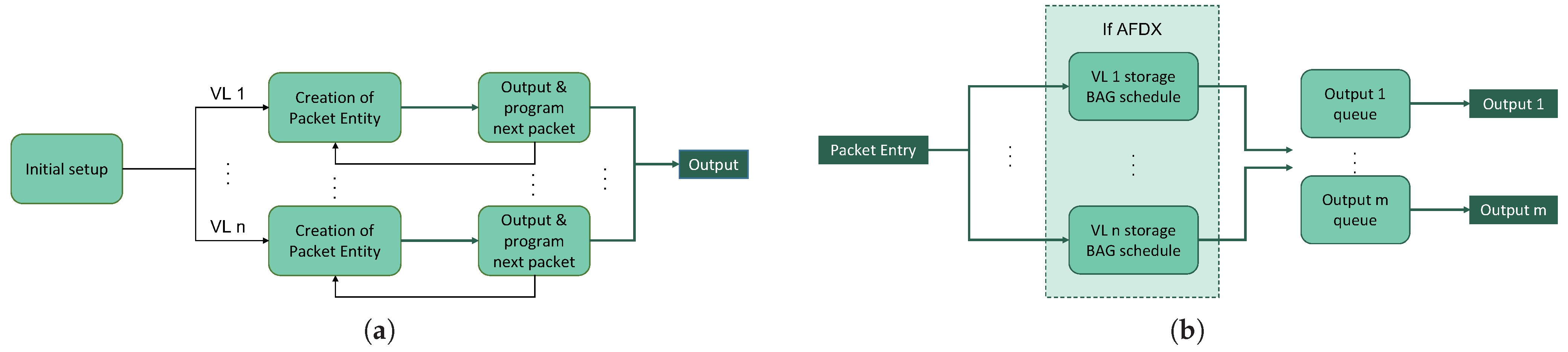
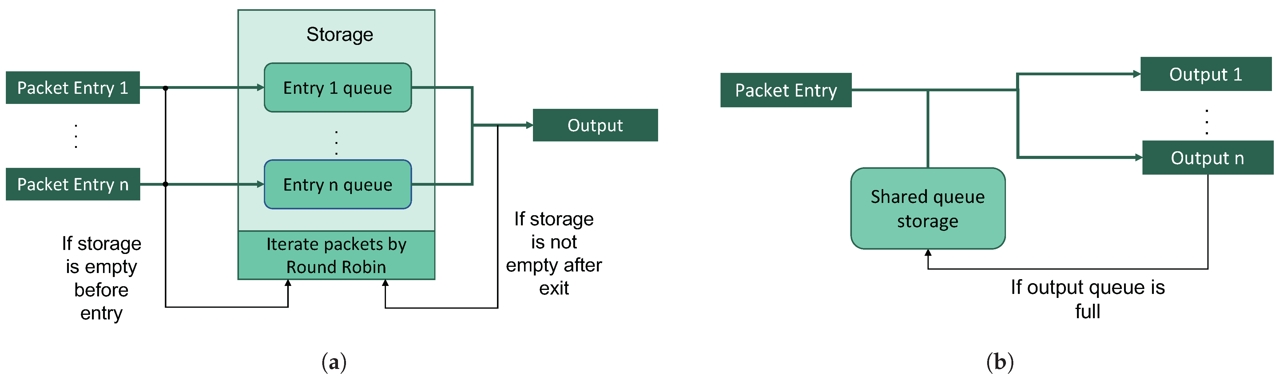
3.3. End System Model
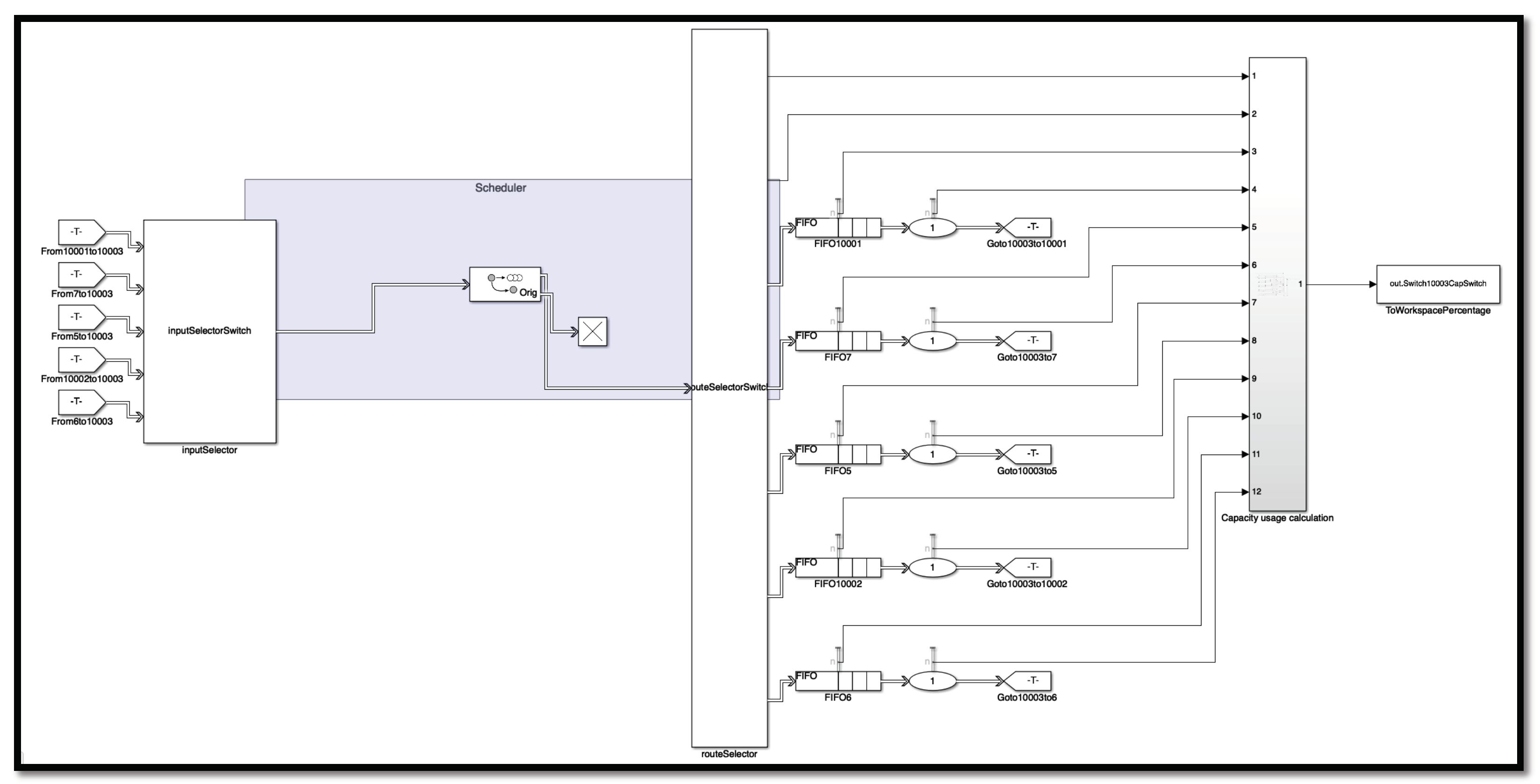
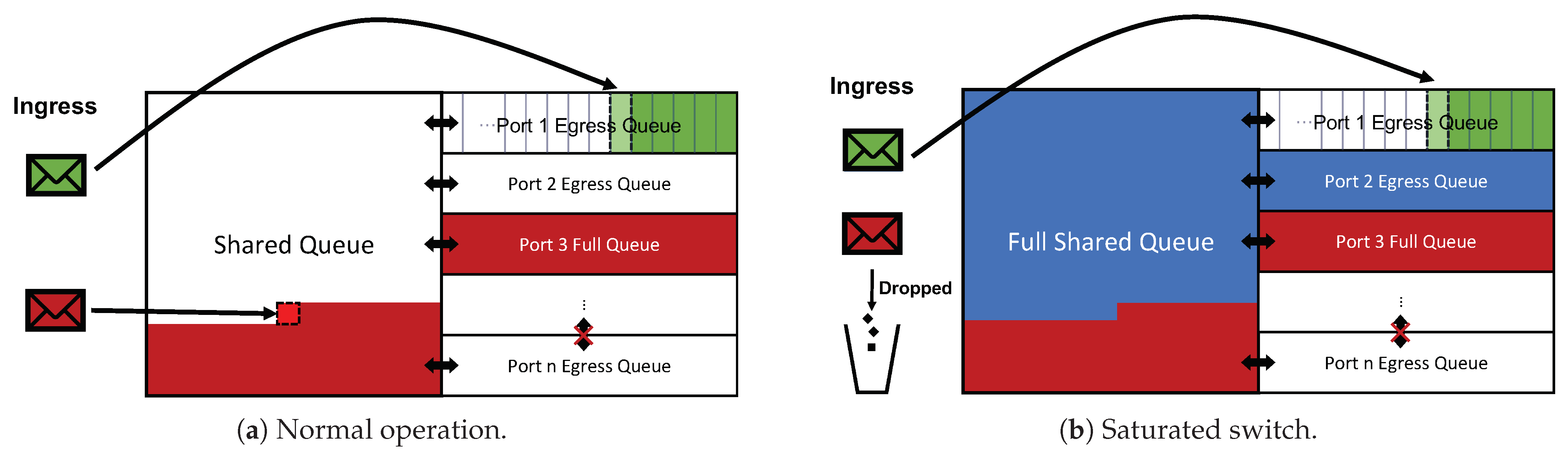
3.4. Switch Model
4. Evaluation
4.1. Correctness of the Results
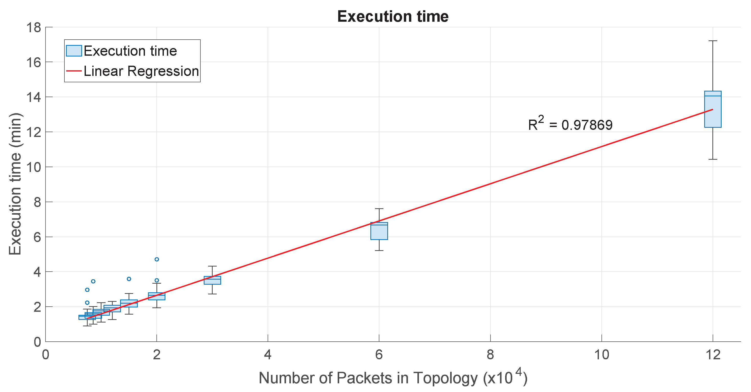
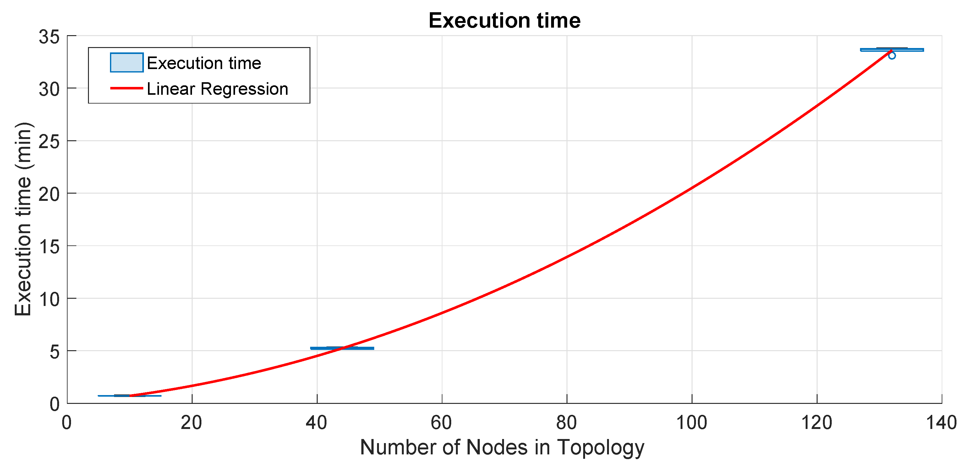
4.2. Computational Performance Analysis
4.3. Results Comparison
5. Discussion
6. Conclusions and Outlook
Author Contributions
Funding
Data Availability Statement
Acknowledgments
Conflicts of Interest
References
- Butz, H. Open Integrated Modular Avionic (IMA): State of the Art and future Development Road Map at Airbus Deutschland. 2008. Available online: https://www.semanticscholar.org/paper/Open-Integrated-Modular-Avionic-(-IMA-)-%3A-State-of-Butz/042d7fc1a86cfd72d8e33f8e2ed93bb7c54a9ffd (accessed on 5 May 2023).
- Brajou, F.; Ricco, P. The Airbus A380—An AFDX-based flight test computer concept. In Proceedings of the AUTOTESTCON 2004, San Antonio, TX, USA, 20–23 September 2004; pp. 460–463. [Google Scholar]
- Boeing. Boeing-777. Available online: https://www.boeing.es/productos-y-servicios/commercial-airplanes/777.page (accessed on 5 May 2023).
- Kazi, S.I. Architecting of Avionics Full Duplex Ethernet (AFDX) Aerospace Communication Network. 2013. Available online: https://www.iject.org/vol4/spl4/c0140.pdf (accessed on 5 May 2023).
- Villegas, J.; Fortes, S.; Escano, V.; Baena, C.; Colomer, B.; Barco, R. Verification and Validation Framework for AFDX Avionics Networks. IEEE Access 2022, 10, 66743–66756. [Google Scholar] [CrossRef]
- Mifdaoui, A.; Amari, A. Real-time ethernet solutions supporting ring topology from an avionics perspective: A short survey. In Proceedings of the 2017 22nd IEEE International Conference on Emerging Technologies and Factory Automation (ETFA), Limassol, Cyprus, 12–15 September 2017; pp. 1–8. [Google Scholar] [CrossRef]
- Amari, A.; Mifdaoui, A. Specification and Performance Indicators of AeroRing—A Multiple-Ring Ethernet Network for Avionics Embedded Systems. Sensors 2018, 18, 3871. [Google Scholar] [CrossRef] [PubMed]
- Doverfelt, R.; Skolan, K.; Elektroteknik, F.; Datavetenskap, O. An Evaluation of Ethernet as Data Transport System in Avionics 2020. Available online: https://www.diva-portal.org/smash/get/diva2:1484743/FULLTEXT01.pdf (accessed on 5 May 2023).
- Deng, L.; Xie, G.; Liu, H.; Han, Y.; Li, R.; Li, K. A Survey of Real-Time Ethernet Modeling and Design Methodologies: From AVB to TSN. ACM Comput. Surv. 2022, 55, 1–36. [Google Scholar] [CrossRef]
- IEEE P802.1DP; TSN for Aerospace Onboard Ethernet Communications. IEEE: Piscataway, NJ, USA, 2023. Available online: https://1.ieee802.org/tsn/802-1dp/ (accessed on 5 May 2023).
- AC 20-152-RTCA; Document RTCA/DO-254, Design Assurance Guidance for Airborne Electronic Hardware—Document Information. Federal Aviation Administration: Washington, DC, USA, 2005.
- DO-178C RTCA; Software Considerations in Airborne Systems and Equipment Certification. Federal Aviation Administration: Washington, DC, USA, 2012.
- IEEE. Welcome to the IEEE 802.1 Working Group. Available online: https://1.ieee802.org/ (accessed on 5 May 2023).
- IEEE. IEEE SA—IEEE 802.1BA-2021. Available online: https://standards.ieee.org/ieee/802.1BA/10547/ (accessed on 5 May 2023).
- IEEE. IEEE SA—IEEE 802.1CMde-2020. Available online: https://standards.ieee.org/ieee/802.1CMde/7478/ (accessed on 5 May 2023).
- IEEE. IEC/IEEE 60802 TSN Profile for Industrial Automation. Available online: https://1.ieee802.org/tsn/iec-ieee-60802/ (accessed on 5 May 2023).
- IEEE. P802.1DG—TSN Profile for Automotive In-Vehicle Ethernet Communications. Available online: https://1.ieee802.org/tsn/802-1dg/ (accessed on 5 May 2023).
- IEEE. IEEE SA—IEEE 802.1Q-2018. Available online: https://standards.ieee.org/ieee/802.1Q/6844/ (accessed on 5 May 2023).
- Mathworks. Solvers for Discrete-Event Systems—MATLAB & Simulink. Available online: https://es.mathworks.com/help/simevents/ug/solvers-for-simevents-models.html (accessed on 20 January 2023).
- Altuntaş, M.; Eker, M.; Kışla, P.; Can, E.; Demir, M.; Hokelek, I.; Akdogan, E. Testing Deterministic Avionics Networks Using Orthogonal Arrays. In Proceedings of the The Fifteenth International Conference on Mobile Ubiquitous Computing, Systems, Services and Technologies, Barcelona, Spain, 3–7 October 2021. [Google Scholar]
- Curtiss-Wright Defense Solutions. Parvus DuraNET 20-10. Available online: https://www.curtisswrightds.com/products/networking-communications/rugged-systems/duranet-20-10 (accessed on 5 May 2023).
- Xu, Q.; Yang, X. Performance Analysis on Transmission Estimation for Avionics Real-Time System Using Optimized Network Calculus. Int. J. Aeronaut. Space Sci. 2019, 20, 506–517. [Google Scholar] [CrossRef]
- Finzi, A.; Mifdaoui, A.; Frances, F.; Lochin, E. Network Calculus-based Timing Analysis of AFDX networks incorporating multiple TSN/BLS traffic classes. arXiv 2019, arXiv:1905.00399. [Google Scholar]


| Parameter | Fields |
|---|---|
| Simulation time | Duration in seconds |
| BER | Bit error rate |
| Topology | Protocol |
| Identifier | |
| ESs | |
| Route A | |
| Route B | |
| Cable length (m) | |
| Link speed (bps) | |
| BAG/periodicity (ms) | |
| Min/max packet length (B) | |
| Switch characteristics (delay and memory) |
| Transmitter | VL | Receiver | Path | Packet Length | BAG |
|---|---|---|---|---|---|
| ES1 | VL1 | ES6 | ES1 → S1 → S3 → ES6 | 500 B | 4 ms |
| ES2 | VL2 | ES7 | ES2 → S1 → S3 → ES7 | 500 B | 4 ms |
| ES3 | VL3 | ES6 | ES3 → S2 → S3 → ES6 | 500 B | 4 ms |
| ES4 | VL4 | ES6 | ES4 → S2 → S3 → ES6 | 500 B | 4 ms |
| ES5 | VL5 | ES6 | ES5 → S3 → ES6 | 500 B | 4 ms |
| Transmission Start | Evaluation Method | |||||||
|---|---|---|---|---|---|---|---|---|
| VL | ES1 | ES2 | ES3 | ES4 | ES5 | EPL | BNCOG | Simulation |
| VL1 | 2 t s | t s | 0 s | 0 s | 96 s | 272 s | 272.8 s | 272 s |
| VL2 | 0 s | t s | 0 s | 0 s | 96 s | 192 s | 192 s | 192 s |
| VL3 | t s | 0 µs | 2 t s | t s | 96 s | 272 s | 272.8 s | 272 s |
| VL4 | t s | 0 s | t s | 2 t s | 96 s | 272 s | 272.8 s | 272 s |
| VL5 | t s | 0 s | 0 s | 0 s | 96 + 2 t s | 176 s | 176.8 s | 176 s |
| Parameter | Fields |
|---|---|
| Simulation time | 1 s |
| Protocol | Ethernet |
| Link speed | 1 Gbps |
| Packet length | 1280 B |
| Periodicity | [0.5, 1, 2, 3, 4, 5, 6, 7, 8] ms |
| Topology | A350 |
| #VLs | 60 |
| Parameter | Fields |
|---|---|
| Simulation time | 0.5 s |
| Protocol | AFDX |
| Link speed | 1 Gbps |
| Packet length | 1280 B |
| BAG | 1 ms |
| #VLs | 3 per ES |
| Timestamp (s) | Delay (s) | Arrival Time (s) | Depart Time (s) | Payload Size (B) | Tx Address | Rx Address | VL | Seq (×1014) | |
|---|---|---|---|---|---|---|---|---|---|
| 1 | 0 | 6.3344 | 1280 | 7 | 1 | 1 | 9.1667 | ||
| 2 | 7.3896 | 6.3344 | 1.0552 | 7.3896 | 1280 | 7 | 1 | 2 | 10.768 |
| 3 | 9.5001 | 6.3344 | 3.1657 | 9.5001 | 1280 | 7 | 1 | 15 | 15.317 |
| 4 | 1.1611 | 6.3344 | 5.2762 | 1.1611 | 1280 | 7 | 1 | 32 | 40.854 |
| 5 | 1.0633 | 6.3344 | 1.0000 | 1.0633 | 1280 | 7 | 1 | 1 | 2.9073 |
| 6 | 1.0738 | 6.3344 | 1.0205 | 1.0738 | 1280 | 7 | 1 | 2 | 4.0522 |
| 7 | 1.0950 | 6.3344 | 1.0316 | 1.0950 | 1280 | 7 | 1 | 15 | 35.144 |
| 8 | 1.1161 | 6.3344 | 1.0527 | 1.1161 | 1280 | 7 | 1 | 32 | 36.255 |
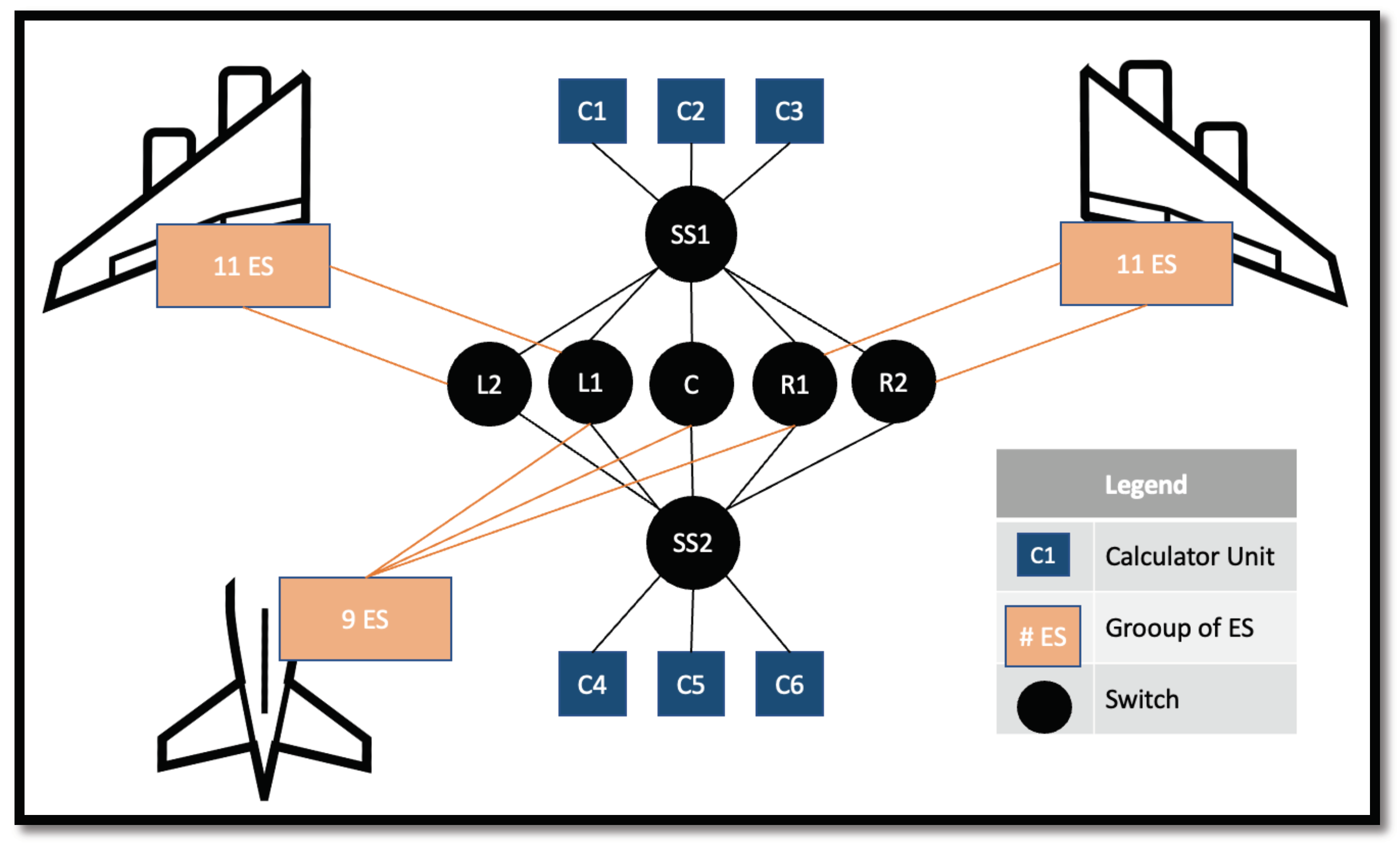
| VL | Transmitter | Receiver | Path | Packet Length | BAG/Periodicity | VL | Transmitter | Receiver | Path | Packet Length | BAG/Periodicity |
|---|---|---|---|---|---|---|---|---|---|---|---|
| VL1 | ES29 | C1 | ES29 R2 SS1 C1 | 1280 B | 1 ms | VL41 | ES30 | C1 | ES30 R2 SS1 C1 | 400 B | 1 ms |
| VL2 | C4 | ES4 | C4 SS2 L2 ES4 | 400 B | 0.5 ms | VL42 | ES26 | C6 | ES26 R2 SS2 C6 | 128 B | 1 ms |
| VL3 | ES17 | C6 | ES17 C SS2 C6 | 512 B | 8 ms | VL43 | ES13 | C2 | ES13 C SS1 C2 | 256 B | 1 ms |
| VL4 | C1 | ES31 | C1 SS1 R2 ES31 | 256 B | 2 ms | VL44 | ES14 | C6 | ES14 C SS2 C6 | 512 B | 8 ms |
| VL5 | C3 | ES25 | C3 SS1 R1 ES25 | 1280 B | 8 ms | VL45 | ES9 | C1 | ES9 L1 SS1 C1 | 1100 B | 0.5 ms |
| VL6 | ES14 | C6 | ES14 C SS2 C6 | 900 B | 8 ms | VL46 | ES27 | C4 | ES27 R2 SS2 C4 | 64 B | 8 ms |
| VL7 | ES30 | C4 | ES30 R2 SS2 C4 | 64 B | 0.5 ms | VL47 | ES5 | C6 | ES5 L2 SS2 C6 | 128 B | 0.5 ms |
| VL8 | ES27 | C6 | ES27 R2 SS2 C6 | 900 B | 1 ms | VL48 | ES11 | C4 | ES11 L1 SS2 C4 | 900 B | 1 ms |
| VL9 | ES24 | C5 | ES24 R1 SS2 C5 | 64 B | 0.5 ms | VL49 | ES3 | C2 | ES3 L2 SS1 C2 | 128 B | 4 ms |
| VL10 | ES21 | C2 | ES21 R1 SS1 C2 | 256 B | 2 ms | VL50 | ES6 | C2 | ES6 L2 SS1 C2 | 512 B | 4 ms |
| VL11 | ES1 | C2 | ES1 L2 SS1 C2 | 900 B | 2 ms | VL51 | ES2 | C6 | ES2 L2 SS2 C6 | 1100 B | 1 ms |
| VL12 | ES4 | C5 | ES4 L2 SS2 C5 | 400 B | 4 ms | VL52 | C3 | ES16 | C3 SS1 C ES16 | 1100 B | 1 ms |
| VL13 | ES10 | C6 | ES10 L1 SS2 C6 | 1100 B | 2 ms | VL53 | ES28 | C3 | ES28 R2 SS1 C3 | 64 B | 4 ms |
| VL14 | ES14 | C3 | ES14 C SS1 C3 | 128 B | 4 ms | VL54 | ES25 | C3 | ES25 R1 SS1 C3 | 1100 B | 2 ms |
| VL15 | ES25 | C2 | ES25 R1 SS1 C2 | 900 B | 4 ms | VL55 | ES13 | C1 | ES13 C SS1 C1 | 256 B | 8 ms |
| VL16 | ES14 | C4 | ES14 C SS2 C4 | 128 B | 4 ms | VL56 | ES30 | C6 | ES30 R2 SS2 C6 | 400 B | 2 ms |
| VL17 | ES24 | C2 | ES24 R1 SS1 C2 | 1280 B | 1 ms | VL57 | ES2 | C2 | ES2 L2 SS1 C2 | 1100 B | 4 ms |
| VL18 | ES21 | C1 | ES21 R1 SS1 C1 | 750 B | 2 ms | VL58 | ES26 | C1 | ES26 R2 SS1 C1 | 256 B | 4 ms |
| VL19 | ES16 | C6 | ES16 C SS2 C6 | 400 B | 8 ms | VL59 | ES6 | C4 | ES6 L2 SS2 C4 | 750 B | 8 ms |
| VL20 | ES19 | C2 | ES19 R1 SS1 C2 | 512 B | 1 ms | VL60 | ES21 | C3 | ES21 R1 SS1 C3 | 750 B | 0.5 ms |
| VL21 | ES8 | C4 | ES8 L1 SS2 C4 | 1280 B | 0.5 ms | VL61 | ES10 | C5 | ES10 L1 SS2 C5 | 750 B | 8 ms |
| VL22 | ES28 | C6 | ES28 R2 SS2 C6 | 900 B | 0.5 ms | VL62 | ES22 | C2 | ES22 R1 SS1 C2 | 900 B | 4 ms |
| VL23 | ES5 | C1 | ES5 L2 SS1 C1 | 1100 B | 2 ms | VL63 | ES20 | C5 | ES20 R1 SS2 C5 | 750 B | 2 ms |
| VL24 | ES27 | C2 | ES27 R2 SS1 C2 | 128 B | 0.5 ms | VL64 | ES29 | C5 | ES29 R2 SS2 C5 | 256 B | 2 ms |
| VL25 | ES8 | C6 | ES8 L1 SS2 C6 | 128 B | 8 ms | VL65 | ES14 | C3 | ES14 C SS1 C3 | 256 B | 0.5 ms |
| VL26 | ES7 | C2 | ES7 L1 SS1 C2 | 1280 B | 2 ms | VL66 | ES16 | C4 | ES16 C SS2 C4 | 400 B | 8 ms |
| VL27 | ES15 | C3 | ES15 C SS1 C3 | 64 B | 2 ms | VL67 | ES25 | C4 | ES25 R1 SS2 C4 | 512 B | 1 ms |
| VL28 | ES19 | C4 | ES19 R1 SS2 C4 | 1280 B | 1 ms | VL68 | ES26 | C4 | ES26 R2 SS2 C4 | 400 B | 4 ms |
| VL29 | C2 | ES24 | C2 SS1 R1 ES24 | 512 B | 8 ms | VL69 | ES30 | C6 | ES30 R2 SS2 C6 | 750 B | 4 ms |
| VL30 | ES12 | C4 | ES12 L1 SS2 C4 | 400 B | 0.5 ms | VL70 | ES20 | C4 | ES20 R1 SS2 C4 | 256 B | 2 ms |
| VL31 | ES2 | C4 | ES2 L2 SS2 C4 | 64 B | 1 ms | VL71 | ES10 | C3 | ES10 L1 SS1 C3 | 400 B | 2 ms |
| VL32 | ES29 | C1 | ES29 R2 SS1 C1 | 750 B | 0.5 ms | VL72 | ES27 | C2 | ES27 R2 SS1 C2 | 1100 B | 4 ms |
| VL33 | ES15 | C1 | ES15 C SS1 C1 | 1100 B | 8 ms | VL73 | ES6 | C2 | ES6 L2 SS1 C2 | 64 B | 8 ms |
| VL34 | ES6 | C5 | ES6 L2 SS2 C5 | 900 B | 0.5 ms | VL74 | ES10 | C6 | ES10 L1 SS2 C6 | 1280 B | 4 ms |
| VL35 | ES17 | C1 | ES17 C SS1 C1 | 750 B | 1 ms | VL75 | ES6 | C6 | ES6 L2 SS2 C6 | 1280 B | 8 ms |
| VL36 | ES9 | C4 | ES9 L1 SS2 C4 | 64 B | 1 ms | VL76 | C3 | ES4 | C3 SS1 L2 ES4 | 512 B | 2 ms |
| VL37 | ES24 | C3 | ES24 R1 SS1 C3 | 750 B | 4 ms | VL77 | ES13 | C4 | ES13 C SS2 C4 | 512 B | 0.5 ms |
| VL38 | ES8 | C6 | ES8 L1 SS2 C6 | 900 B | 8 ms | VL78 | ES19 | C5 | ES19 R1 SS2 C5 | 128 B | 1 ms |
| VL39 | ES26 | C4 | ES26 R2 SS2 C4 | 512 B | 0.5 ms | VL79 | ES4 | C2 | ES4 L2 SS1 C2 | 64 B | 4 ms |
| VL40 | C1 | ES14 | C1 SS1 C ES14 | 1280 B | 2 ms | VL80 | ES14 | C4 | ES14 C SS2 C4 | 256 B | 0.5 ms |
| VL | Delay (µs) | Jitter (µs) | Throughput (Kbps) | Packet Loss (%) | VL | Delay (µs) | Jitter (µs) | Throughput (Kbps) | Packet Loss (%) | ||||
|---|---|---|---|---|---|---|---|---|---|---|---|---|---|
| Mean | Std | Mean | Std | Mean | Std | Mean | Std | ||||||
| 1 | 5246.1 | 683.19 | 253.21 | 634.5 | 1717.1 | 20.842 | 41 | 5159.3 | 671.83 | 238.07 | 628.21 | 1717.1 | 6.0666 |
| 2 | 105.57 | 5.1888 | 1.9086 | 4.8249 | 130.8 | 0 | 42 | 336.27 | 164.01 | 136.55 | 90.807 | 130.8 | 0.65524 |
| 3 | 376.63 | 154.67 | 128.68 | 85.426 | 284.95 | 1.2245 | 43 | 171.04 | 95.664 | 73.45 | 61.27 | 284.95 | 0.050429 |
| 4 | 80.376 | 5.438 | 5.4246 | 3.4102 | 332.75 | 0 | 44 | 379.1 | 161.01 | 131.04 | 93.183 | 332.75 | 2.3166 |
| 5 | 252.42 | 0.14869 | 0.018622 | 0.14751 | 220.58 | 0.3937 | 45 | 5238 | 651.23 | 236.15 | 606.89 | 220.58 | 17.863 |
| 6 | 450.96 | 159.33 | 132.89 | 87.466 | 350.55 | 1.2448 | 46 | 5065 | 328.19 | 85.074 | 316.93 | 350.55 | 4.2969 |
| 7 | 5079.3 | 232.52 | 79.154 | 218.63 | 1774.3 | 3.5661 | 47 | 334.78 | 163.41 | 135.8 | 90.877 | 1774.3 | 0.39448 |
| 8 | 434.56 | 156.75 | 130.2 | 87.224 | 360.87 | 2.2959 | 48 | 5175.4 | 323.96 | 94.756 | 309.78 | 360.87 | 43.489 |
| 9 | 66.762 | 28.359 | 22.739 | 16.943 | 278.82 | 0 | 49 | 156.93 | 95.261 | 75.865 | 57.513 | 278.82 | 0 |
| 10 | 175.72 | 94.467 | 73.892 | 58.809 | 902.75 | 0.10121 | 50 | 219.92 | 95.22 | 75.732 | 57.617 | 902.75 | 0 |
| 11 | 273.02 | 89.147 | 68.386 | 57.147 | 212.54 | 0.30738 | 51 | 461.48 | 155.32 | 129.52 | 85.688 | 212.54 | 3.0153 |
| 12 | 125.4 | 29.706 | 24.834 | 16.263 | 1052.3 | 0 | 52 | 222.24 | 0.77226 | 0.15096 | 0.75736 | 1052.3 | 0 |
| 13 | 459.12 | 150.28 | 125.6 | 82.409 | 78.884 | 3.4161 | 53 | 68.718 | 30.636 | 23.826 | 19.228 | 78.884 | 0 |
| 14 | 83.284 | 37.041 | 28.161 | 24.029 | 484.62 | 0 | 54 | 238.55 | 25.889 | 19.565 | 16.943 | 484.62 | 0 |
| 15 | 273.62 | 93.307 | 72.391 | 58.785 | 73.192 | 0 | 55 | 5116 | 720.05 | 276.48 | 664.62 | 73.192 | 4.6512 |
| 16 | 5088.1 | 274.15 | 83.657 | 261.05 | 2598.3 | 6.8762 | 56 | 372.66 | 158.25 | 130.5 | 89.416 | 2598.3 | 1.8127 |
| 17 | 323.19 | 87.64 | 67.082 | 56.378 | 680.97 | 0.15068 | 57 | 307.16 | 99.28 | 73.571 | 66.583 | 680.97 | 0.38462 |
| 18 | 5215.2 | 635.2 | 225.04 | 593.95 | 101.74 | 12.475 | 58 | 5128.7 | 688.91 | 252.31 | 640.93 | 101.74 | 4.2857 |
| 19 | 361.68 | 162.62 | 134.49 | 90.998 | 1065.7 | 0.41841 | 59 | 5135.5 | 506.11 | 136.84 | 487.13 | 1065.7 | 40.249 |
| 20 | 210.25 | 94.524 | 72.41 | 60.737 | 2415.3 | 0.05048 | 60 | 176.83 | 27.085 | 18.578 | 19.707 | 2415.3 | 0.025233 |
| 21 | 5198.5 | 384.58 | 115.22 | 366.91 | 3529.2 | 51.888 | 61 | 184.73 | 29.439 | 24.547 | 16.176 | 3529.2 | 0 |
| 22 | 433.59 | 157.57 | 131.8 | 86.326 | 873.18 | 2.3584 | 62 | 269.89 | 88.026 | 66.646 | 57.43 | 873.18 | 0.1938 |
| 23 | 5226.4 | 714.1 | 265.19 | 662.96 | 604.05 | 22.577 | 63 | 180.14 | 25.908 | 21.136 | 14.969 | 604.05 | 0 |
| 24 | 155.28 | 97.908 | 76.265 | 61.386 | 35.878 | 0.02551 | 64 | 99.826 | 29.231 | 23.326 | 17.602 | 35.878 | 0 |
| 25 | 336.43 | 171.81 | 141.43 | 97.109 | 1300.2 | 0.8547 | 65 | 100.9 | 32.568 | 25.072 | 20.783 | 1300.2 | 0 |
| 26 | 331.4 | 86.477 | 66.28 | 55.505 | 91.133 | 0.1004 | 66 | 5104.6 | 381.03 | 97.424 | 368.3 | 91.133 | 19.672 |
| 27 | 70.835 | 32.715 | 25.578 | 20.381 | 1128.5 | 0 | 67 | 5123.2 | 322.39 | 95.251 | 307.99 | 1128.5 | 25.92 |
| 28 | 5205.2 | 407.25 | 117.75 | 389.83 | 135.48 | 56.148 | 68 | 5106.9 | 356.87 | 101.34 | 342.14 | 135.48 | 20.468 |
| 29 | 123.38 | 6.0004 | 5.9264 | 8.611 | 1347.5 | 0.39841 | 69 | 409.57 | 156.21 | 128.67 | 88.373 | 1347.5 | 2.5794 |
| 30 | 5118.1 | 267.17 | 84.246 | 253.54 | 173.47 | 19.11 | 70 | 5093 | 335.08 | 95.365 | 321.2 | 173.47 | 13.636 |
| 31 | 5081.8 | 233.7 | 78.755 | 220.02 | 2682.9 | 3.8423 | 71 | 126.88 | 34.304 | 25.984 | 22.381 | 2682.9 | 0 |
| 32 | 5199 | 658.93 | 243.02 | 612.46 | 226.51 | 11.231 | 72 | 302.71 | 93.6 | 73.386 | 58.002 | 226.51 | 0 |
| 33 | 5234.2 | 702.61 | 256.02 | 654.05 | 3667.2 | 19.679 | 73 | 150.84 | 106.29 | 78.409 | 71.58 | 3667.2 | 0 |
| 34 | 195.6 | 17.139 | 10.603 | 13.464 | 1367.5 | 0.025259 | 74 | 490.67 | 153.7 | 130.98 | 80.197 | 1367.5 | 3.5785 |
| 35 | 5190.8 | 685.53 | 254.66 | 636.44 | 171.8 | 12.475 | 75 | 513.11 | 158.11 | 131.68 | 87.093 | 171.8 | 4.5082 |
| 36 | 5085.7 | 219.69 | 75.663 | 206.24 | 388.56 | 3.443 | 76 | 125.95 | 7.3683 | 4.3839 | 5.9207 | 388.56 | 0.099701 |
| 37 | 185.76 | 34.521 | 26.466 | 22.133 | 220.48 | 0 | 77 | 5131.2 | 275.03 | 85.297 | 261.46 | 220.48 | 23.711 |
| 38 | 447.78 | 141.19 | 116.29 | 79.72 | 1618.2 | 3.2653 | 78 | 79.191 | 29.744 | 23.919 | 17.672 | 1618.2 | 0 |
| 39 | 5127.2 | 272.66 | 87.871 | 258.11 | 1300.2 | 24.085 | 79 | 136.55 | 91.567 | 71.269 | 57.406 | 1300.2 | 0.19342 |
| 40 | 252.5 | 0.80937 | 0.18706 | 0.78743 | 805.38 | 0 | 80 | 5097 | 262.88 | 82.952 | 249.44 | 805.38 | 12.598 |
| VL | Delay (µs) | Jitter (µs) | Throughput (Kbps) | Packet Loss (%) | VL | Delay (µs) | Jitter (µs) | Throughput (Kbps) | Packet Loss (%) | ||||
|---|---|---|---|---|---|---|---|---|---|---|---|---|---|
| Mean | Std | Mean | Std | Mean | Std | Mean | Std | ||||||
| 1 | 482.37 | 93.349 | 85.696 | 36.918 | 852.43 | 49.135 | 41 | 104.57 | 3.525 | 2.6026 | 2.3759 | 852.43 | 49.9 |
| 2 | 104.57 | 3.5776 | 2.6058 | 2.4507 | 67.792 | 49.571 | 42 | 67.393 | 19.032 | 12.782 | 14.095 | 67.792 | 50.348 |
| 3 | 147.86 | 3.1272 | 2.6501 | 1.6431 | 141.28 | 51.923 | 43 | 84.785 | 8.9162 | 6.8199 | 5.7394 | 141.28 | 50.025 |
| 4 | 80.376 | 5.7043 | 5.4875 | 1.5381 | 164.57 | 50.642 | 44 | 629.21 | 1.3022 | 7.185 | 1.0841 | 164.57 | 50.98 |
| 5 | 252.41 | 2.139 | 1.8294 | 1.0962 | 116.67 | 50.98 | 45 | 267.02 | 71.414 | 61.674 | 35.976 | 116.67 | 48.24 |
| 6 | 307.9 | 9.3641 | 2.3405 | 9.0644 | 180.09 | 48.56 | 46 | 242.68 | 6.5281 | 5.3866 | 3.6561 | 180.09 | 50.98 |
| 7 | 70.213 | 42.853 | 25.281 | 34.596 | 927.04 | 49.686 | 47 | 258.81 | 144.7 | 124.66 | 73.411 | 927.04 | 49.837 |
| 8 | 195.46 | 18.465 | 11.904 | 14.111 | 180.09 | 49.975 | 48 | 226.48 | 11.359 | 7.5097 | 8.5194 | 180.09 | 49.52 |
| 9 | 48.12 | 5.5794 | 4.3391 | 3.5061 | 141.28 | 50.199 | 49 | 58.872 | 1.2788 | 6.7322 | 1.0864 | 141.28 | 48.665 |
| 10 | 95.673 | 10.969 | 10.488 | 3.1775 | 463.93 | 48.454 | 50 | 463.99 | 1.0155 | 9.8199 | 2.513 | 463.93 | 51.55 |
| 11 | 261.31 | 41.462 | 41.391 | 1.547 | 106.93 | 49.749 | 51 | 423.17 | 85.785 | 77.395 | 36.92 | 106.93 | 49.29 |
| 12 | 104.57 | 3.5217 | 2.5894 | 2.3812 | 564.2 | 49.698 | 52 | 222.17 | 4.117 | 3.4699 | 2.2129 | 564.2 | 49.469 |
| 13 | 417.69 | 52.239 | 45.195 | 26.119 | 38.655 | 52.153 | 53 | 48.12 | 5.0921 | 4.2708 | 2.7598 | 38.655 | 49.084 |
| 14 | 60.69 | 4.9127 | 4.0216 | 2.81 | 232.43 | 51.644 | 54 | 287.17 | 3.7347 | 3.0937 | 2.0877 | 232.43 | 49.341 |
| 15 | 377.89 | 43.828 | 23.733 | 36.816 | 38.656 | 48.98 | 55 | 112.02 | 4.3846 | 3.1502 | 3.0365 | 38.656 | 51.362 |
| 16 | 234.36 | 20.932 | 20.89 | 6.4511 | 1307.8 | 51.362 | 56 | 285.58 | 52.239 | 45.195 | 26.119 | 1307.8 | 50.397 |
| 17 | 394.07 | 158.52 | 141.67 | 70.996 | 388.79 | 48.533 | 57 | 729.67 | 3.7325 | 3.725 | 1.2011 | 388.79 | 51.172 |
| 18 | 174.96 | 13.82 | 11.59 | 7.5105 | 53.679 | 50.1 | 58 | 90.987 | 10.632 | 10.611 | 6.4576 | 53.679 | 48.98 |
| 19 | 104.57 | 3.5487 | 2.5998 | 2.4042 | 538.56 | 47.699 | 59 | 530.47 | 6.2479 | 5.1852 | 3.4546 | 538.56 | 50.593 |
| 20 | 137.26 | 13.949 | 13.594 | 3.0973 | 2613.7 | 50.372 | 60 | 163.37 | 3.0549 | 2.5627 | 1.6618 | 2613.7 | 49.393 |
| 21 | 355.56 | 52.685 | 45.964 | 25.73 | 1853.3 | 46.921 | 61 | 212.58 | 5.356 | 4.4554 | 2.9456 | 1853.3 | 49.597 |
| 22 | 260.41 | 98.178 | 58.265 | 79.008 | 564.15 | 48.901 | 62 | 244.54 | 44.922 | 26.724 | 36.069 | 564.15 | 49.9 |
| 23 | 288.1 | 13.82 | 11.59 | 7.5105 | 308.21 | 48.98 | 63 | 165.13 | 1.7668 | 1.765 | 3.2911 | 308.21 | 50.348 |
| 24 | 120.66 | 83.379 | 75.969 | 34.32 | 19.405 | 50.311 | 64 | 122.2 | 28.074 | 24.256 | 14.092 | 19.405 | 49.85 |
| 25 | 518.02 | 1.2485 | 5.5473 | 1.1173 | 654.41 | 50.593 | 65 | 128.48 | 0.017723 | 0.0085781 | 0.015508 | 654.41 | 50.483 |
| 26 | 416.81 | 78.787 | 78.708 | 8.8648 | 45.09 | 49.9 | 66 | 147.77 | 5.0018 | 4.159 | 2.7535 | 45.09 | 48.347 |
| 27 | 48.12 | 6.8471 | 4.5613 | 5.1025 | 1307.5 | 49.799 | 67 | 411.38 | 56.666 | 42.811 | 37.1 | 1307.5 | 50.298 |
| 28 | 459.82 | 38.586 | 31.124 | 22.787 | 67.792 | 48.901 | 68 | 381.96 | 20.932 | 20.89 | 4.4607 | 67.792 | 50 |
| 29 | 123.38 | 5.9998 | 5.9148 | 8.552 | 852.43 | 55.986 | 69 | 543.22 | 66.678 | 66.545 | 1.0492 | 852.43 | 52.107 |
| 30 | 117.2 | 37.82 | 21.845 | 30.869 | 90.09 | 50.087 | 70 | 190.88 | 14.88 | 12.874 | 7.4401 | 90.09 | 49.393 |
| 31 | 53.387 | 5.2872 | 4.6456 | 2.52 | 1553.4 | 49.316 | 71 | 273.81 | 31.196 | 31.165 | 4.3855 | 1553.4 | 49.597 |
| 32 | 317.79 | 139.49 | 121.39 | 68.673 | 141.89 | 49.058 | 72 | 642.91 | 3.5798 | 3.5726 | 1.0965 | 141.89 | 49.698 |
| 33 | 442.32 | 45.171 | 44.815 | 3.975 | 1853 | 50.199 | 73 | 470 | 1.0382 | 1.0236 | 1.4718 | 1853 | 50.397 |
| 34 | 201.29 | 22.061 | 19.086 | 11.057 | 776.98 | 48.546 | 74 | 594.77 | 125.61 | 125.36 | 9.6547 | 776.98 | 47.146 |
| 35 | 334.17 | 93.349 | 85.696 | 36.918 | 90.09 | 49.85 | 75 | 824.52 | 1.2254 | 5.9082 | 1.0723 | 90.09 | 48.133 |
| 36 | 57.529 | 5.2167 | 4.5133 | 2.6122 | 194.78 | 49.52 | 76 | 123.38 | 5.9724 | 5.907 | 8.4126 | 194.78 | 48.718 |
| 37 | 311.53 | 4.2774 | 3.6576 | 2.2055 | 116.68 | 50.593 | 77 | 203.22 | 49.976 | 44.179 | 23.342 | 116.68 | 49.367 |
| 38 | 685.4 | 1.2464 | 6.4195 | 1.0668 | 1076.5 | 48.56 | 78 | 88.746 | 35.875 | 29.874 | 19.841 | 1076.5 | 49.444 |
| 39 | 160.49 | 37.82 | 21.845 | 30.869 | 654.31 | 49.774 | 79 | 77.521 | 2.7128 | 2.5423 | 9.3295 | 654.31 | 52.471 |
| 40 | 252.41 | 2.1124 | 1.797 | 1.1074 | 426.43 | 50.249 | 80 | 272.93 | 109.07 | 98.943 | 45.847 | 426.43 | 49.52 |
Disclaimer/Publisher’s Note: The statements, opinions and data contained in all publications are solely those of the individual author(s) and contributor(s) and not of MDPI and/or the editor(s). MDPI and/or the editor(s) disclaim responsibility for any injury to people or property resulting from any ideas, methods, instructions or products referred to in the content. |
© 2024 by the authors. Licensee MDPI, Basel, Switzerland. This article is an open access article distributed under the terms and conditions of the Creative Commons Attribution (CC BY) license (https://creativecommons.org/licenses/by/4.0/).
Share and Cite
Vera-Soto, P.; Villegas, J.; Fortes, S.; Pulido, J.; Escaño, V.; Ortiz, R.; Barco, R. An Event-Driven Link-Level Simulator for the Validation of AFDX and Ethernet Avionics Networks. Aerospace 2024, 11, 247. https://doi.org/10.3390/aerospace11040247
Vera-Soto P, Villegas J, Fortes S, Pulido J, Escaño V, Ortiz R, Barco R. An Event-Driven Link-Level Simulator for the Validation of AFDX and Ethernet Avionics Networks. Aerospace. 2024; 11(4):247. https://doi.org/10.3390/aerospace11040247
Chicago/Turabian StyleVera-Soto, Pablo, Javier Villegas, Sergio Fortes, José Pulido, Vicente Escaño, Rafael Ortiz, and Raquel Barco. 2024. "An Event-Driven Link-Level Simulator for the Validation of AFDX and Ethernet Avionics Networks" Aerospace 11, no. 4: 247. https://doi.org/10.3390/aerospace11040247