
Design and Analysis of the Two-Impulse Transfer Orbit for a Space-Based Gravitational Wave Observatory
Abstract
:1. Introduction
2. Dynamic Model
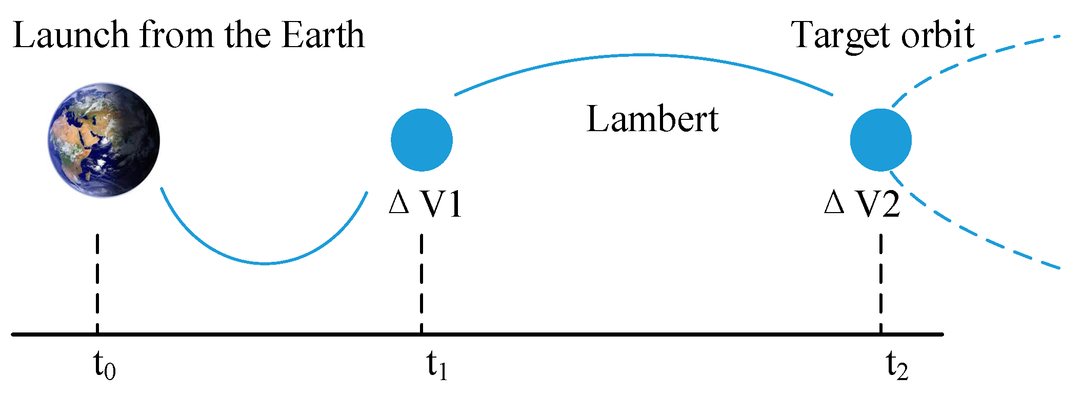
2.1. Two-Impulse Transfer Orbit Model for Space-Based Gravitational Wave Observatory
2.2. Formation Flying Model of the Space-Based Gravitational Wave Observatory
2.3. Constraints on Formation Design for Space-Based Gravitational Wave Observatory
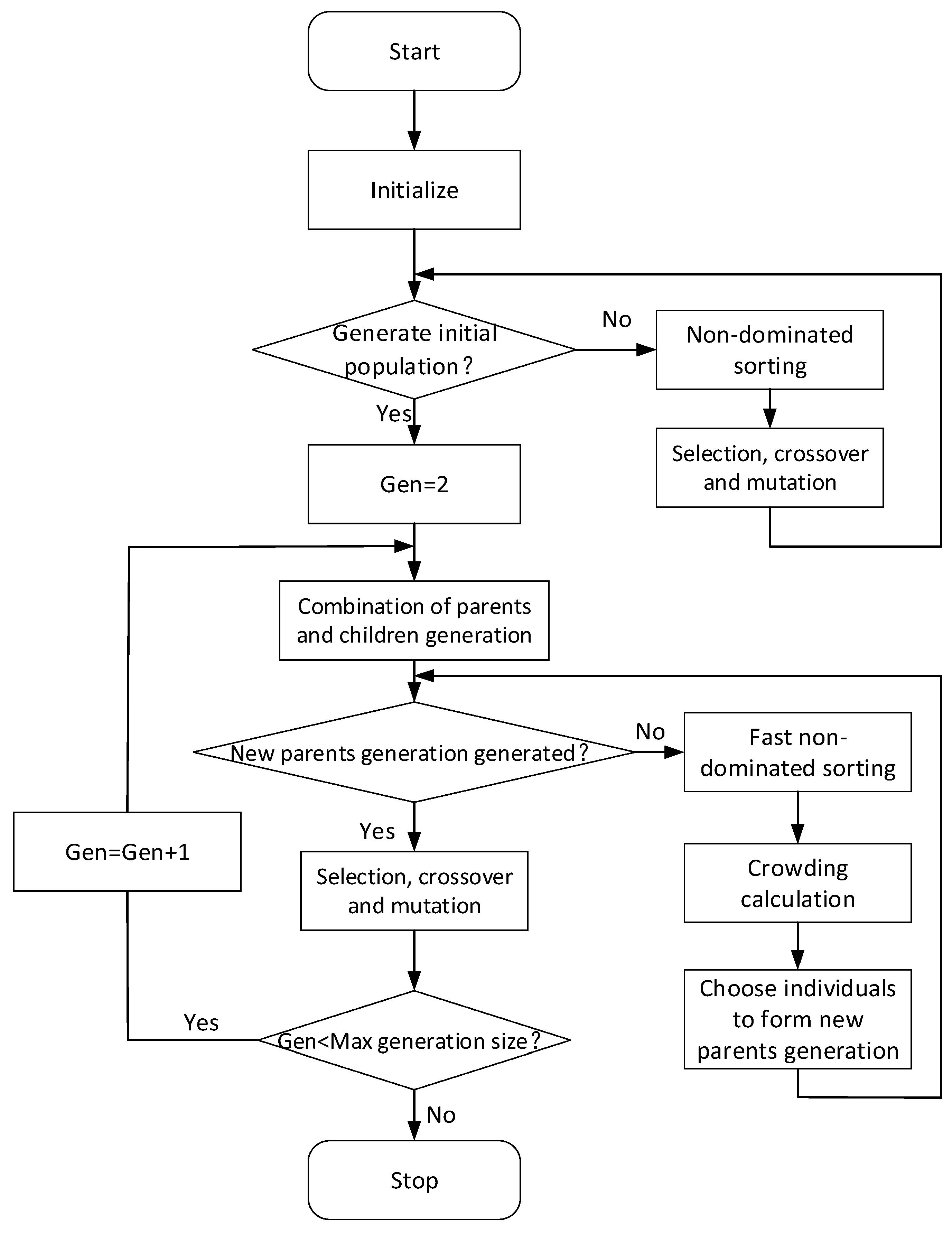
3. Principle of NSGA-II Algorithm
- Step 1: Parameters are initialized, and a random initial population Pt of size N is generated within the specified search range. t represents the tth population and Pt (t = 0) is the parent population.
- Step 2: Non-dominated sorting and basic genetic operations of the parent population Pt are carried out to produce the offspring population Qt.
- Step 3: The parent and offspring populations are combined to create a new population of size 2N. Non-dominated sorting is conducted, the crowding distance is calculated, and elitism is performed to select a new parent population of size N for the generation of the next population. We make t = t + 1.
- Step 4: Selection, crossover, and mutation of the new parent population are performed. Once this is done, we check if the maximum number of evolutions has been reached. If it is, we end the process and take the last population as the optimal solution. Otherwise, we repeat the process from Step 3.
4. Simulation and Analysis
4.1. Selection of Optimization Objectives
4.2. Two-Impulse Transfer Orbit Simulation
4.3. Analysis of Factors Affecting Transfer Orbit Design
- (1)
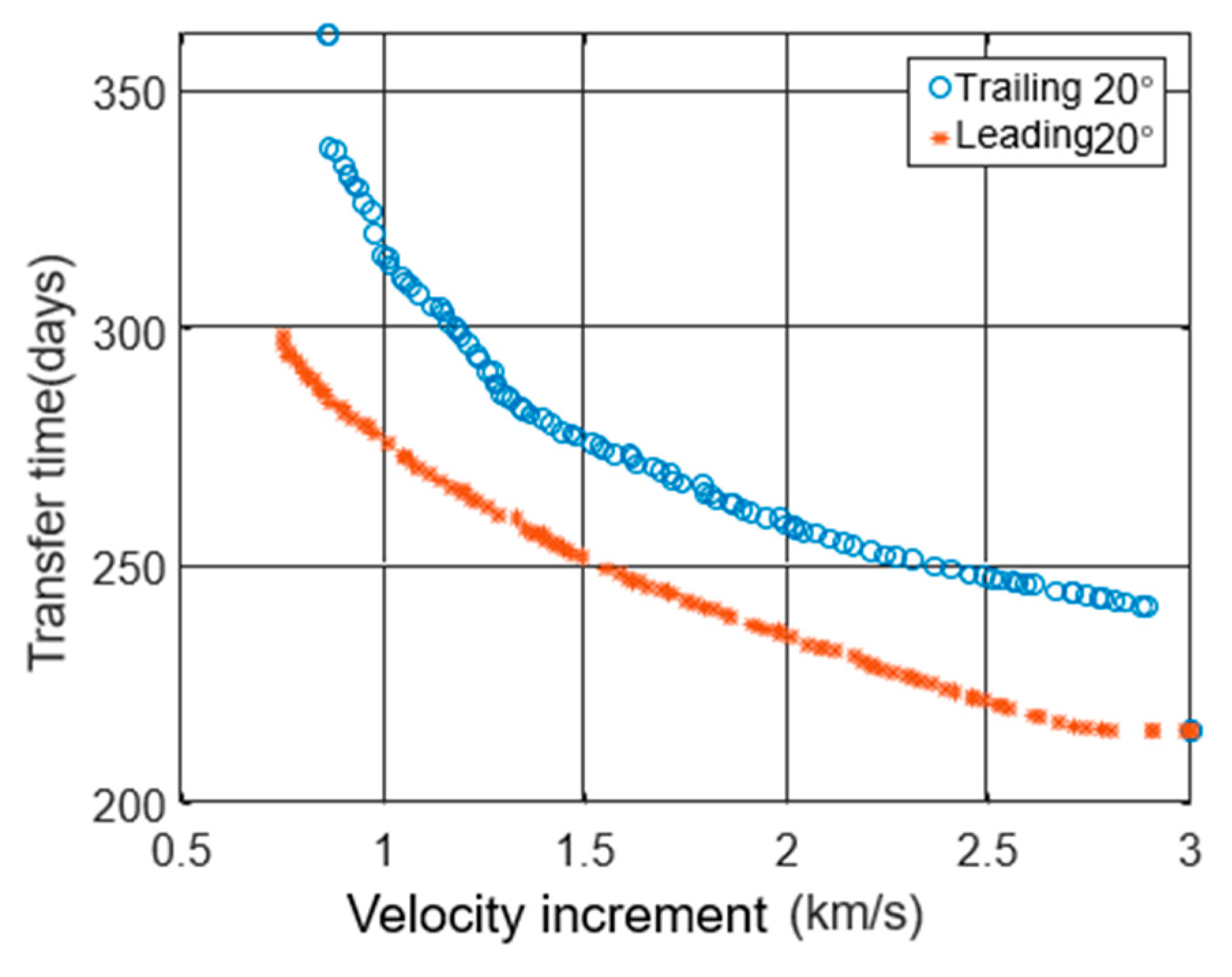
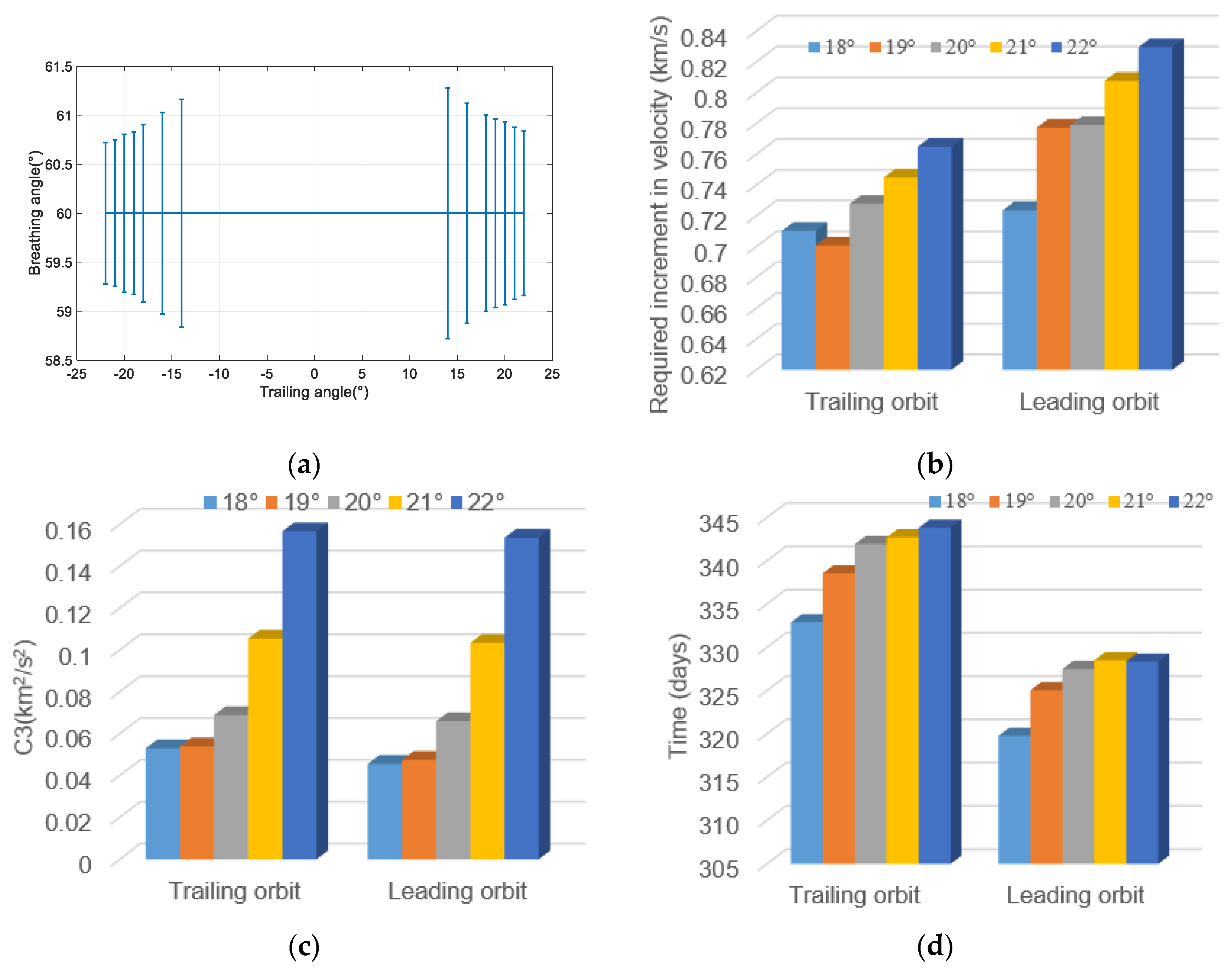
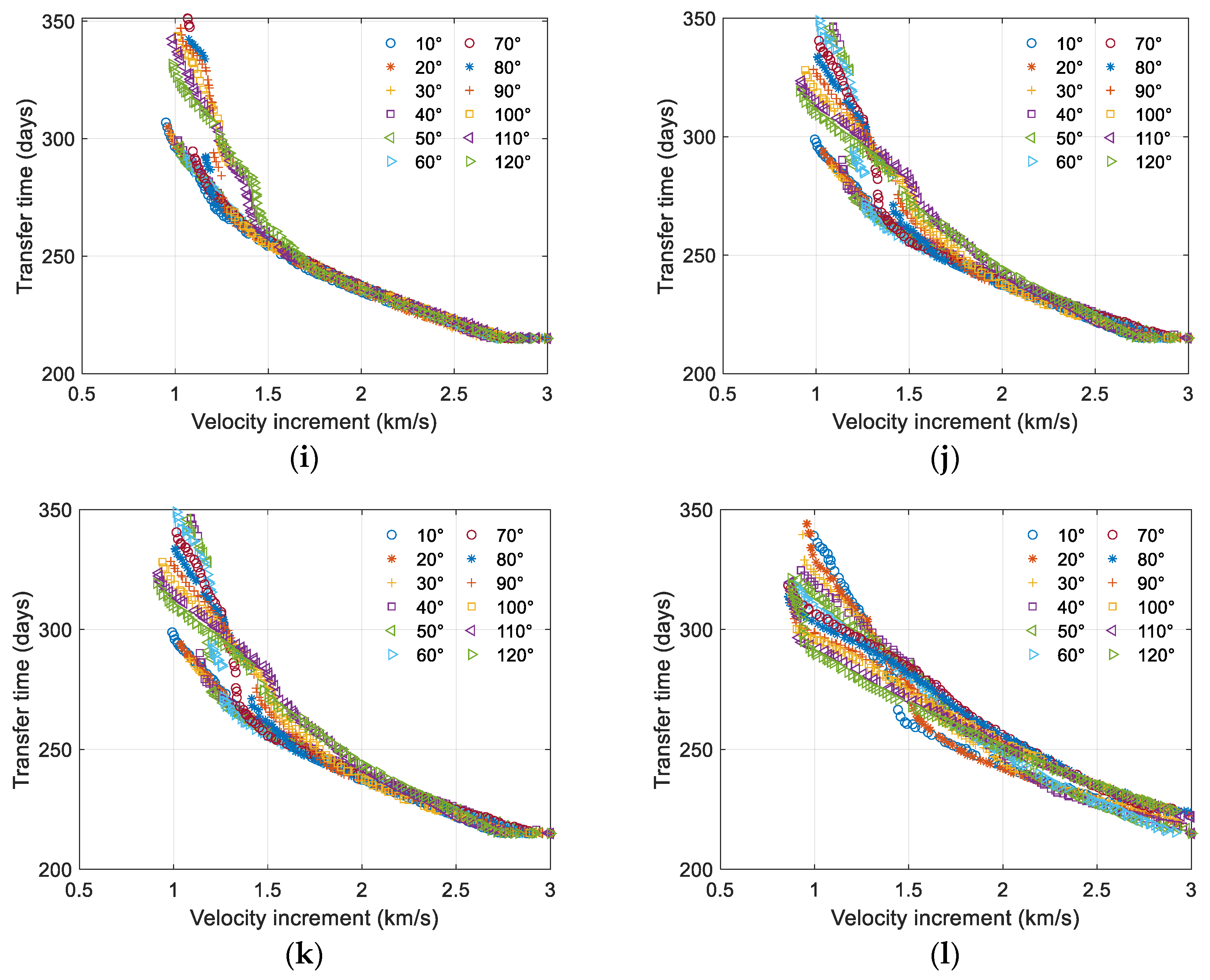
- The effect of the initial trailing angle on the transfer orbit
- (2)
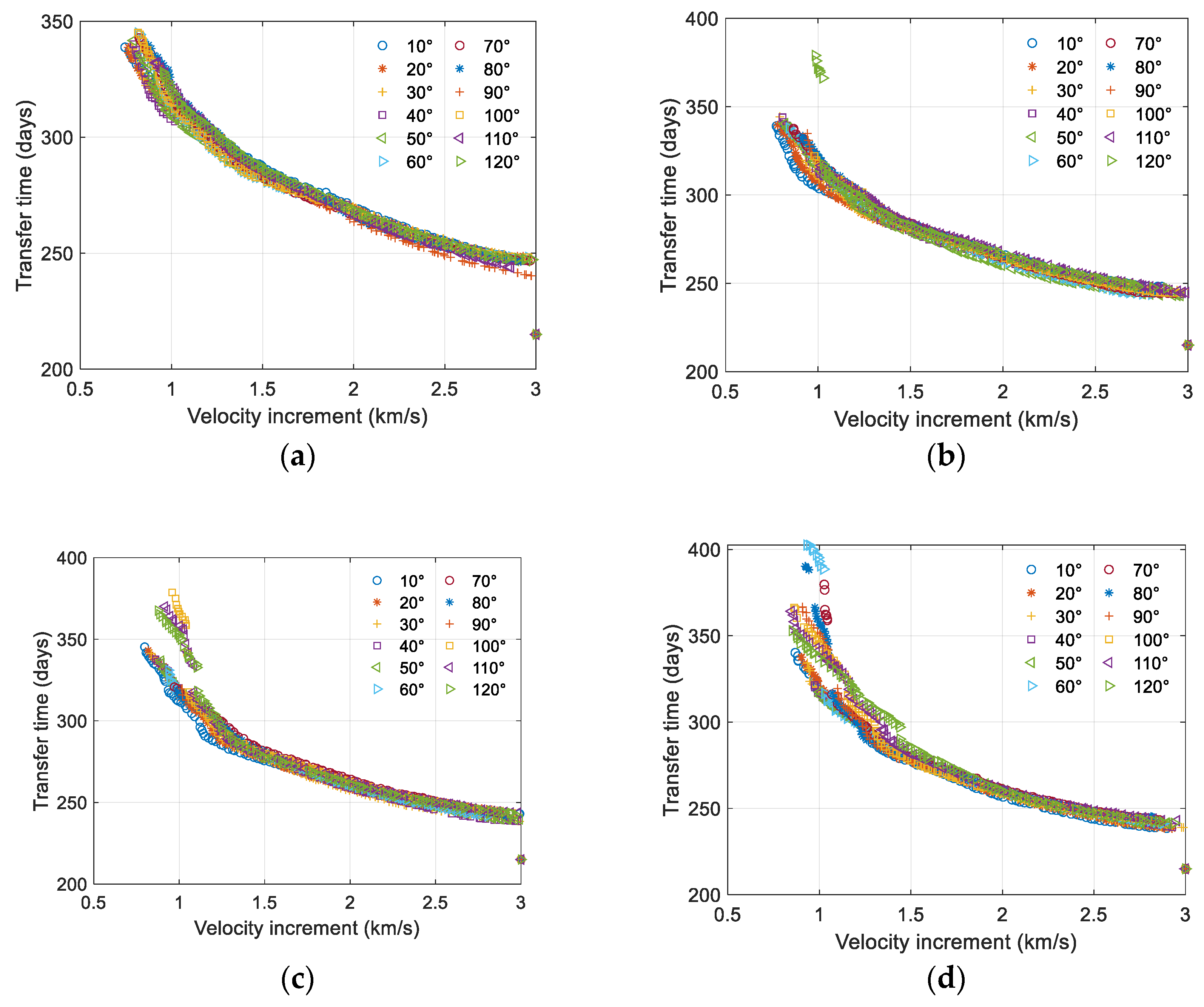
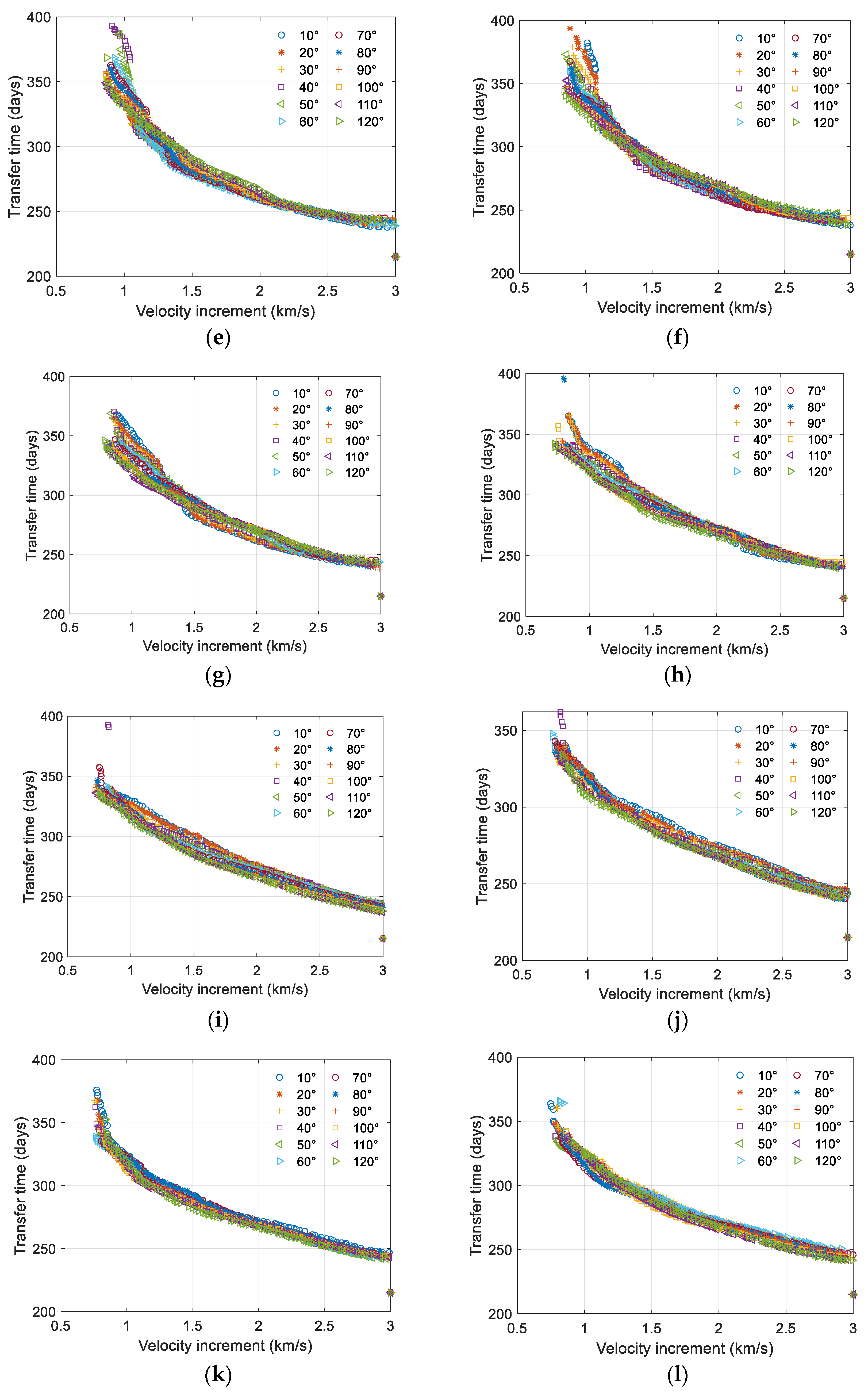
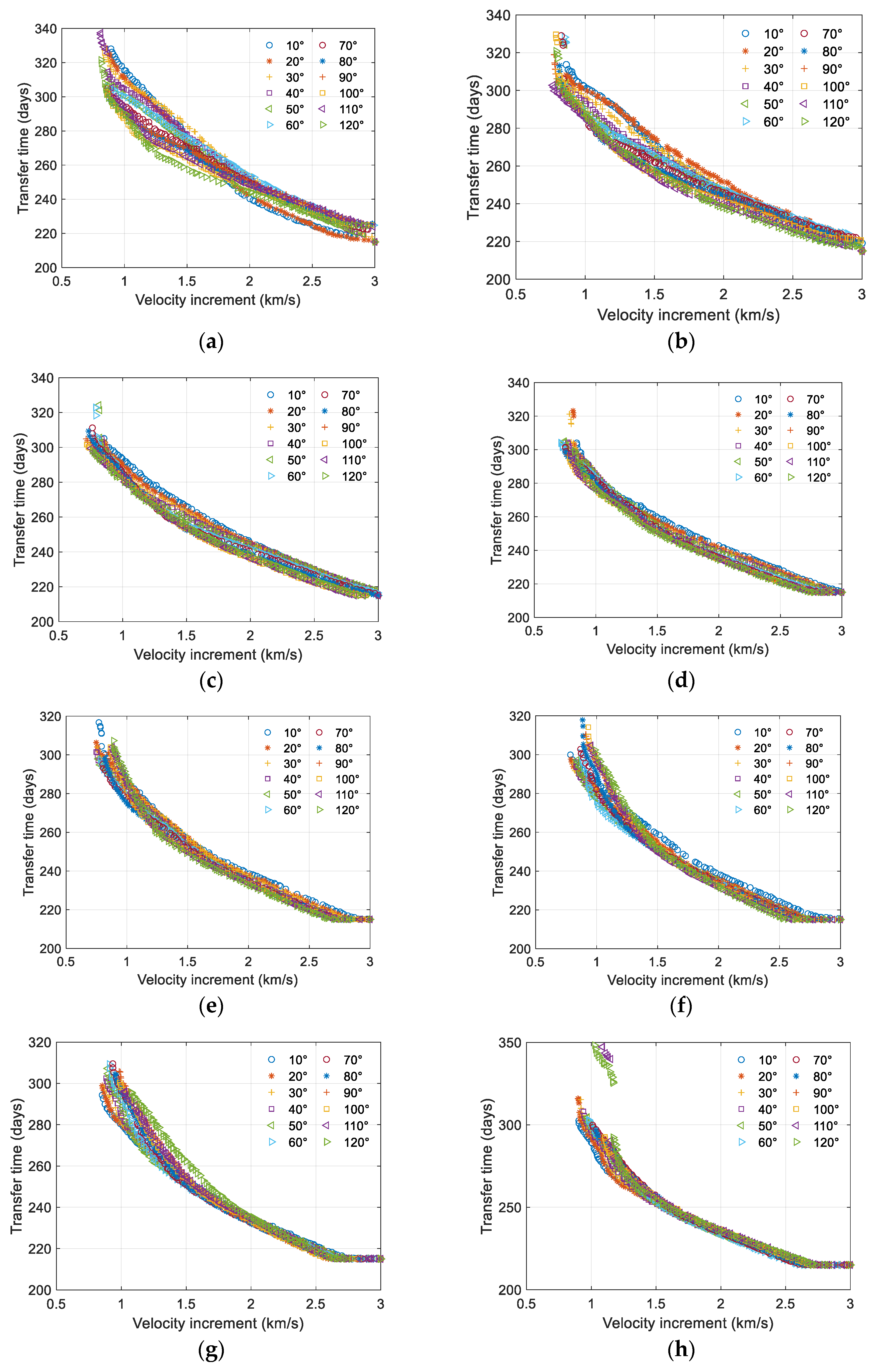
- The effect of the initial phase angle of the formation on the transfer orbit
- (3)
- The effect of the initial time of transfer on the transfer orbit
5. Conclusions
- (1)
- The influence of the initial phase angle of the formation on the transfer orbit.
- (2)
- The effect of the initial time of transfer on the transfer orbit.
- (3)
- The impact of the initial trailing angle on the transfer orbit.
Author Contributions
Funding
Data Availability Statement
Conflicts of Interest
Appendix A


References
- Abbott, B.P.; Abbott, R.; Adhikari, R.; Ajith, P.; Allen, B.; Allen, G.; Amin, R.S.; Anderson, S.B.; Anderson, W.G.; A Arain, M.; et al. LIGO: The laser interferometer gravitational-wave observatory. Rep. Prog. Phys. 2009, 72, 7. [Google Scholar] [CrossRef]
- Abbott, B.P.; Abbott, R.; Abbott, T.D.; Acernese, F.; Ackley, K.; Adams, C.; Adams, T.; Addesso, P.; Adhikari, R.X.; Adya, V.B.; et al. GW170817: Implications for the stochastic gravitational-wave background from compact binary coalescences. Phys. Rev. Lett. 2018, 120, 091101. [Google Scholar] [CrossRef] [PubMed]
- Cornish, N.J.; Rubbo, L.J. LISA response function. Phys. Rev. D 2003, 67, 022001. [Google Scholar] [CrossRef]
- Nayak, K.R.; Koshti, S.; Dhurandhar, S.V.; Vinet, J.Y. On the minimum flexing of LISA’s arms. Class. Quantum Gravity 2006, 23, 1763. [Google Scholar] [CrossRef]
- Pucacco, G.; Bassan, M.; Visco, M. Autonomous perturbations of LISA orbits. Class. Quantum Gravity 2010, 27, 235001. [Google Scholar] [CrossRef]
- Li, G.; Yi, Z.; Heinzel, G.; Rüdiger, A.; Jennrich, O.; Wang, L.; Xia, Y.; Zeng, F.; Zhao, H. Methods for Orbit Optimization for the Lisa Gravitational Wave Observatory. Int. J. Mod. Phys. D 2008, 17, 1021–1042. [Google Scholar] [CrossRef]
- Li, Z.; Zheng, J. Orbit determination for a space-based gravitational wave observatory. Acta Astronaut. 2021, 185, 170–178. [Google Scholar] [CrossRef]
- Li, Z.; Zheng, J.; Li, M. Orbit insertion error analysis for a space-based gravitational wave observatory. Adv. Space Res. 2020, 67, 3744–3754. [Google Scholar] [CrossRef]
- Luo, Z.; Guo, Z.; Jin, G.; Wu, Y.; Hu, W. A brief analysis to Taiji: Science and technology. Results Phys. 2019, 16, 102918. [Google Scholar] [CrossRef]
- Luo, Z.; Liu, H.; Jin, G. The recent development of interferometer prototype for Chinese gravitational wave detection pathfinder mission. Opt. Laser Technol. 2018, 105, 146–151. [Google Scholar] [CrossRef]
- Mei, J.; Bai, Y.-Z.; Bao, J.; Barausse, E.; Cai, L.; Canuto, E.; Cao, B.; Chen, W.-M.; Chen, Y.; Ding, Y.-W.; et al. The TianQin project: Current progress on science and technology. Prog. Theor. Exp. Phys. 2020, 2021, 05A107. [Google Scholar] [CrossRef]
- Liang, Z.-C.; Hu, Y.-M.; Jiang, Y.; Cheng, J.; Zhang, J.-D.; Mei, J. Science with the TianQin Observatory: Preliminary results on stochastic gravitational-wave background. Phys. Rev. D 2022, 105, 022001. [Google Scholar] [CrossRef]
- Ye, B.-B.; Zhang, X.; Zhou, M.-Y.; Wang, Y.; Yuan, H.-M.; Gu, D.; Ding, Y.; Zhang, J.; Mei, J.; Luo, J. Optimizing orbits for TianQin. Int. J. Mod. Phys. D 2019, 28, 1950121. [Google Scholar] [CrossRef]
- Hu, X.-C.; Li, X.-H.; Wang, Y.; Feng, W.-F.; Zhou, M.-Y.; Hu, Y.-M.; Hu, S.-C.; Mei, J.-W.; Shao, C.-G. Fundamentals of the orbit and response for TianQin. Class. Quantum Gravity 2018, 35, 095008. [Google Scholar] [CrossRef]
- Tan, Z.; Ye, B.; Zhang, X. Impact of orbital orientations and radii on TianQin constellation stability. Int. J. Mod. Phys. D 2020, 29, 2050056. [Google Scholar] [CrossRef]
- Xia, Y.; Li, G.; Heinzel, G.; Rüdiger, A.; Luo, Y. Orbit design for the Laser Interferometer Space Antenna (LISA). Sci. China Phys. Mech. Astron. 2010, 53, 179–186. [Google Scholar] [CrossRef]
- Sweetser, T.H. An end-to-end trajectory description of the LISA mission. Class. Quantum Gravity 2005, 22, S429–S435. [Google Scholar] [CrossRef]
- Joffre, E.; Wealthy, D.; Fernandez, I.; Trenkel, C.; Voigt, P.; Ziegler, T.; Martens, W. LISA: Heliocentric formation design for the laser interferometer space antenna mission. Adv. Space Res. 2020, 67, 3868–3879. [Google Scholar] [CrossRef]
- Wang, G.; Ni, W.T.; Wu, A.M. Orbit design and thruster requirement for various constant arm space mission concepts for gravitational-wave observation. Int. J. Mod. Phys. D 2020, 29, 1940006. [Google Scholar] [CrossRef]
- Wu, A.-M.; Ni, W.-T. Deployment and simulation of the ASTROD-GW formation. Int. J. Mod. Phys. D 2013, 22, 1341005. [Google Scholar] [CrossRef]
- Hellings, R. JPL Team X Space-Based Gravitational Wave Observatory OMEGA Report; Califormia Institute of Technogy: Los Angeles, CA, USA, 2012. [Google Scholar]
- Giulicchi, L.; Wu, S.-F.; Fenal, T. Attitude and orbit control systems for the LISA Pathfinder mission. Aerosp. Sci. Technol. 2013, 24, 283–294. [Google Scholar] [CrossRef]
- Zhang, J.; Dai, H.; Dang, Z.; Yue, X. Research on configuration design and initialization method of near-Earth gravitational wave formation. Chin. J. Appl. Mech. 2023, 40, 1249–1256. [Google Scholar]


| (km/s) | (km/s) | (km/s) | Toal Velocity Increments (km/s) | Transfer Time (Days) | |
|---|---|---|---|---|---|
| J1 | 0.6971 | 0.8388 | 0.4800 | 2.0160 | 384.7769 |
| J2 | 1.1260 | 1.1260 | 1.1260 | 3.3780 | 356.7949 |
| J3 | 0.7994 | 0.7994 | 0.5871 | 2.1861 | 390.6246 |
| Constraints | Value |
|---|---|
| Escape velocity increment | 0.1~0.6 km/s |
| Escape azimuth angle | 0~360° |
| Escape pitch angle | −19.5~19.5° |
| Coasting time | 15~150 days |
| Lambert transfer time | 200~400 days |
| Initial phase angle of the formation | 0~180° |
| C3 | (km/s) | (km/s) | (km/s) | Transfer Time (Days) | |
|---|---|---|---|---|---|
| Trailing 20° | 0.1044 | 0.8582 | 0.8581 | 0.8527 | 362.0399 |
| Leading 20° | 0.3084 | 0.7482 | 0.7250 | 0.7487 | 298.4096 |
Disclaimer/Publisher’s Note: The statements, opinions and data contained in all publications are solely those of the individual author(s) and contributor(s) and not of MDPI and/or the editor(s). MDPI and/or the editor(s) disclaim responsibility for any injury to people or property resulting from any ideas, methods, instructions or products referred to in the content. |
© 2024 by the authors. Licensee MDPI, Basel, Switzerland. This article is an open access article distributed under the terms and conditions of the Creative Commons Attribution (CC BY) license (https://creativecommons.org/licenses/by/4.0/).
Share and Cite
Li, Z.; Ling, H.; Zhao, X. Design and Analysis of the Two-Impulse Transfer Orbit for a Space-Based Gravitational Wave Observatory. Aerospace 2024, 11, 234. https://doi.org/10.3390/aerospace11030234
Li Z, Ling H, Zhao X. Design and Analysis of the Two-Impulse Transfer Orbit for a Space-Based Gravitational Wave Observatory. Aerospace. 2024; 11(3):234. https://doi.org/10.3390/aerospace11030234
Chicago/Turabian StyleLi, Zhuo, Huixiang Ling, and Xiao Zhao. 2024. "Design and Analysis of the Two-Impulse Transfer Orbit for a Space-Based Gravitational Wave Observatory" Aerospace 11, no. 3: 234. https://doi.org/10.3390/aerospace11030234