Online Learning-Based Surrogate Modeling of Stratospheric Airship Solar Array Output Power

Abstract

The stratospheric airship is a type of aerostat that uses solar energy as its power source and can fly continuously for months or even years in near space. The rapid and accurate prediction of the output power of its solar array is the key to maintaining energy balance and extending flight time. This paper establishes an online learning model for predicting the output power of the solar array of stratospheric airships. The readings of radiometers arranged on the surface of the airship are used as features for training the model. The parameters of the model can be updated in real-time during the flight process without retraining the entire model. The effect of radiometer placement on the model accuracy was also analyzed. The results show that for the continuous flight of 40 days, the online learning model can achieve an accuracy of 88% after training with 10 days of flight data and the accuracy basically reaches its highest level after 20 days. In addition, placing the radiometers at the four corners of the array can achieve a higher prediction accuracy of 95%. The online model can also accurately identify and reflect the effect of module efficiency attenuation or damage and maintain high accuracy.

1. Introduction

Stratospheric airships are a type of high-altitude aerostat that uses lighter-than-air gas as a lifting source and will drift with local wind or must expend energy to fight it. Stratospheric airships use a cyclic energy system, which primarily consists of a photovoltaic (PV) array, a DC/DC converter with maximum power point tracking (MPPT) functionality, and energy storage batteries to provide the energy required for flight, and can fly continuously for months or even years. Stratospheric airships have a high flight altitude, long float time, wide coverage, and monitoring range. Thus, they can be used for broad applications, such as communication relay, meteorological observation, and disaster warning [1,2,3]. Stratospheric airships can also be used to form intelligent networked unmanned systems, further expanding their application range [4]. Many technological powerhouses around the world are actively promoting the research and verification of stratospheric airship-related technologies [5,6,7,8].

Due to the current low conversion efficiency of solar cells and the low energy density of energy storage batteries, the energy balance of stratospheric airships during flight can only be maintained weakly and is easily broken, which is also the main challenge faced by stratospheric airships during long-term flight. Since the solar array provides all the energy required for airship flight, accurately and quickly predicting the output power of the array is critical to maintaining the energy balance of the airship.

In the initial research on the output characteristics of solar arrays, some scholars only focused on the influence of irradiation distribution on the output power of the solar array. For instance, Wang et al. [9] and Shi et al. [10] initially proposed a numerical computational method for assessing the solar radiation distribution on the PV array of a stratospheric airship. However, as research has increased in intensity, many studies have established high-precision simulation models for calculating the output power of stratospheric airship solar arrays. Sun et al. [11] discussed existing photovoltaic modeling methods and divided them into circuit models, engineering models, and fitting models, providing a reference for selecting appropriate modeling methods based on the requirements for model accuracy and application scenarios. Pande et al. [12] analyzed the impact of solar cell output characteristics and operating conditions of different material systems on the size of solar non-rigid airships. Tang et al. [13] discussed the numerical calculation method for the output power of solar cell arrays in the optimization process of stratospheric airships. Song et al. [14] considered the output characteristics of solar arrays under non- maximum power point tracking (MPPT) mode, which further improved the accuracy of the array power generation model. Liu et al. [15] calculated the non-uniform irradiation and temperature in the solar array of a stratospheric airship and established a simulation model to analyze the mismatch loss of the array under different flight conditions. Shan et al. [16] found that changes in the yaw and pitch angles of stratosphere airships are the main cause of solar array mismatch loss. In addition to reducing the maximum output power, mismatch losses can also mislead the MPPT process, further reducing the actual output power. Liu et al. [17] proposed a solar array output power model that includes the insulation layer structure and analyzed the relationship between the thickness of the insulation layer and the array output power. Zhu et al. [18] studied the effect of thermal effects on the output energy of the solar array on stratosphere airships and found that the temperature difference of photovoltaic modules at different positions in the array is significant, and the output power is significantly reduced compared with that without thermal effects.

In order to further enhance the energy acquisition during the operation of airships, some researchers are focusing on the design of flight strategies and attitude planning. Zhang et al. [19] proposed an attitude angle planning strategy that integrates roll, yaw, and pitch controls to enhance the energy production of PV arrays and the wind resistance of airships. In addition, another factor cannot be ignored—namely shading (which is due to the installation of the top equipment or the flight attitude of the platform). Some existing research findings can serve as references for analyzing this issue. Belhachat et al. [20] conducted a comprehensive analysis of the output characteristics of solar arrays under shading conditions, summarized the reconstruction strategies of photovoltaic arrays, and evaluated the advantages and disadvantages of different methods. Venkateswari et al. [21] further tested and verified various shading situations by building a testing device.

For the application of traditional simulation models mentioned above, in order to improve model accuracy, it is necessary to consider more influencing factors during the modeling process and add more components according to the actual situation. This will inevitably increase the complexity of the model, leading to higher computational resource consumption. In recent years, data-driven surrogate modeling methods have been used more and more frequently. Surrogate models are machine learning methods that use sensor datasets to obtain a corresponding relationship through a certain learning method. The models are trained using only input–output data and do not involve calculating parameters, thereby greatly reducing run time. Surrogate models include two forms of offline learning and online learning. Offline learning divides the dataset into training and testing sets and obtains a model for prediction after training and testing. After the training is completed, the parameters in the model will be fixed. If new data types appear, the dataset needs to be imported to retrain the model. Online learning uses streaming data for training. By continuously sending newly generated data for training, the model is continuously refined, and the relevant parameters can be continuously updated. Currently, many studies use online learning models to solve real-time prediction problems in many fields. Luo et al. [22] applied online incremental learning methods to precipitation nowcasting to adapt to real-time changes in precipitation data. Wu et al. [23] proposed an online adaptation framework based on surrogate learning to deal with concept drift problems in time series prediction in the energy field. Compared with offline models, the accuracy was improved by more than 50%. Lu et al. [24] proposed a flight training data prediction model based on incremental learning, which also provided high prediction accuracy and exceptional real-time performance. Liu et al. [25] used online learning methods to update model parameters in the prediction of solar power generation, thereby avoiding the need for the entire retraining process and having the ability to maintain and enhance accuracy. Kraemer et al. [26] used online machine learning methods to predict indoor photovoltaic energy within 24 h and found that simple machine learning methods are much better than persistence predictors. Puah et al. [27] used a regression unsupervised incremental learning algorithm to predict solar irradiance, and incremental learning enables the model to address climate change and has good long-term predictive performance.

Regarding the solar array of a stratospheric airship, during its flight, the solar cells may experience attenuation or damage due to continuous exposure to sunlight, the aging of the film, hot spots, or wind vibration, which can lead to a decrease in conversion efficiency. If the model is not corrected to a certain extent, such errors will continue to accumulate and affect the prediction accuracy of the model. Online learning methods can effectively avoid this issue.

This paper proposes a surrogate modeling method based on online learning to predict the output power of the solar array on a stratospheric airship during flight. All the data required for training come from sensors mounted on the stratospheric airship itself, and the trained model can accurately predict the output power and adapt to abnormal states such as photovoltaic module attenuation or damage. Moreover, since the model consumes fewer computational resources, it can run on the stratospheric airship computers and provide guidance for autonomous flight. Section 1 introduces the relevant background. Section 2 introduces the online learning model and derives the relevant formulas. Section 3 describes the process of training the online model, including specific parameters and data processing. Section 4 presents the results and analyzes. Section 5 is the conclusion.

2. Model Derivation

Considering that the online learning process is carried out on airship computers with limited computational resources, classification and regression models with lower complexity are needed to reduce power consumption. After comparing multiple models, the use of Naive Bayes classifiers and linear regression models balanced the prediction accuracy and complexity of the surrogate model in a better manner.

2.1. Gaussian Naive Bayes Classifier

The Naive Bayes classifier is a statistical generative model whose parameter estimation process is based on frequency statistics. It classifies data by Bayesian probability estimation and only needs to calculate the conditional probability distribution of the sample set to make predictions. It does not involve loss function optimization. The Naive Bayes classifier assumes that each feature is independent. Its advantages are fast training and good performance for high-dimensional and large-scale datasets. It has been proven to perform surprisingly well with very little training data [28], while most other classifiers, especially artificial neural networks, find these data insufficient. For problems with continuous variable features, Gaussian Naive Bayes classifiers can be used, which assume that the feature distribution follows a Gaussian distribution. The mean and variance are calculated over the entire training set. When using Gaussian Naive Bayes classifiers for prediction, the model uses these parameters to estimate the conditional probability.

The idea of the Naive Bayes classifier is to calculate the posterior probability of each response category under the current input feature conditions. The largest one is used as the predicted category. The specific process is as follows:

Suppose a classification problem contains n features and m categories.

$$X=(X_1,X_2,\cdots ,X_n)$$

(1)

$$y=\left\{y_1,y_2,\cdots ,y_m\right\}$$

(2)

According to Bayesian theory, the posterior probability of a feature is represented by the following equation:

$$P(y\left|X\right.)=\frac{P(X\left|y\right.)P(y)}{P(X)}$$

(3)

Due to the prior assumption that the features are independent of each other, the above equation can be written as:

$$P(y\left|X\right.)=\frac{P(X_1,X_2,\cdots ,X_n\left|y\right.)P(y)}{P(X_1,X_2,\cdots ,X_n)}=\frac{P(y){\displaystyle \prod _{i=1}^{n}P(X_i\left|y\right.)}}{{\displaystyle \prod _{i=1}^{n}P(X_i)}}$$

(4)

where the denominator involves only the features of the input and is independent of the class, which can be simplified to mean that the final class output only needs to compare the size of the numerator. Thus, the expression for the result of the classification prediction is

$$\widehat{y}=\arg \underset{y}{\max }P(y){\displaystyle \prod _{i=1}^{n}P(X_i\left|y\right.)}$$

(5)

In a Gaussian plain Bayes classifier, the conditional probability of each feature is assumed to follow a Gaussian distribution.

$$P(X_i\left|y\right.)\sim G({\mu }_y,{\sigma }_y^2)$$

(6)

Its greatest likelihood estimate is:

$$P(X_i\left|y\right.)=\frac{1}{\sqrt{2\pi {\sigma }_y^2}}\exp \left(-\frac{{(X_i-{\mu }_y)}^2}{2{\sigma }_y^2}\right)$$

(7)

The mean and variance in the above equation are obtained by counting the data corresponding to the training set.

It should be noted that for online learning, since training and prediction are continuously performed, the mean and variance are dynamically calculated as the training samples flow in.

2.2. Linear Regression Model

The idea of the linear regression model is to use a linear function to describe the relationship between the independent variable and the dependent variable. Then, according to the error between the predicted value and the actual value, the loss function is defined, and the weights in the function are calculated by minimizing the loss function.

It is assumed that the response to a regression problem consists of two parts. One part is affected by the features and the other part is affected by other factors, which can be considered as a kind of random error. Therefore, the model can be expressed as:

$$\widehat{y}=f\left(x_1,x_2\cdots x_n\right)+b$$

(8)

Linear regression models consider the relationship between features and response as a linear function.

$$\widehat{y}=w_0+w_1{x}_1+\cdots +w_n{x}_n+b={\displaystyle \sum _{i=1}^n{w}_i{x}_i}+b=w^T·x+b$$

(9)

In fact, the random error term can be merged into the zero-weight term. Thus, the loss function is defined as:

$$L(w)=\frac{1}{2}{\left(\widehat{y}-y\right)}^2=\frac{1}{2}{\left(w^T·x+b-y\right)}^2$$

(10)

The weights are calculated as:

$$w=\arg \underset{w}{\min }L\left(w\right)=\arg \underset{w}{\min }\frac{1}{2}{\left(w^T·x+b-y\right)}^2$$

(11)

It should be noted that the formulas above are applicable to online learning, and only the current input sample is used to calculate the loss function, without retaining previous sample information. This form can be conveniently used to calculate weights using stochastic gradient descent. The weights are updated by continuously receiving individual new samples from the data stream, which can be understood as dividing the entire optimization problem into several independent sub-problems and combining the optimal solution of each sub-problem to obtain the optimal solution of the entire problem.

2.3. Online Learning Model

Online learning models are implemented using the River library in Python, which is a Python framework specifically designed for online incremental learning. It can handle data streams and dynamically train machine learning models. The established online learning model includes steps of data preprocessing, feature engineering, and parameter updating.

Data preprocessing: Since the relevant features and responses for training online models are collected through sensors arranged on the stratosphere airship, there may be problems such as abnormal, missing, or duplicate data. It is necessary to perform data cleaning on the training samples in advance to ensure the accuracy and consistency of the data.

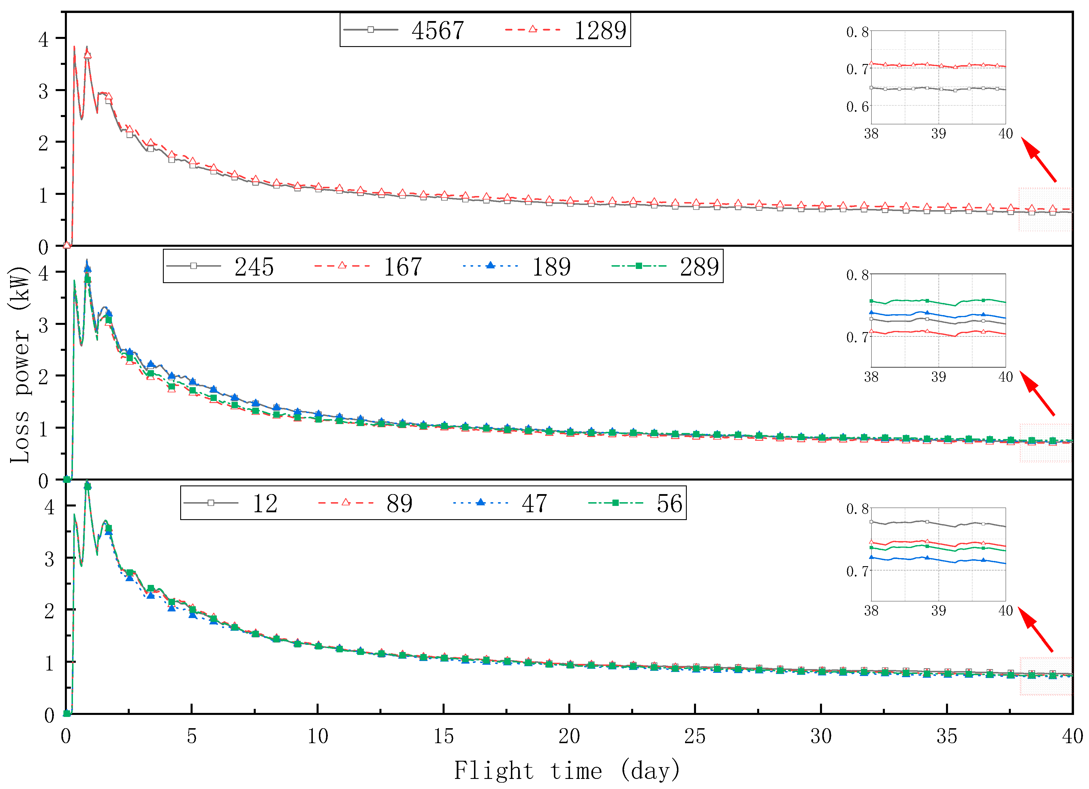
Feature engineering: Feature engineering refers to the process of transforming or selecting original collected samples. Its purpose is to remove redundant features with low impact to improve model performance. In general, many factors will affect the response that needs to be predicted, and there are complex coupling effects between each factor. If all influencing factors are sent to the model for training, it will inevitably increase the complexity of the model and consume more computing resources. In addition, too many features will increase the risk of overfitting. When the number of features exceeds the actual information, the model may learn noise or irrelevant features in the data. This will cause the model to have high accuracy in the training set but poor accuracy in the new data.

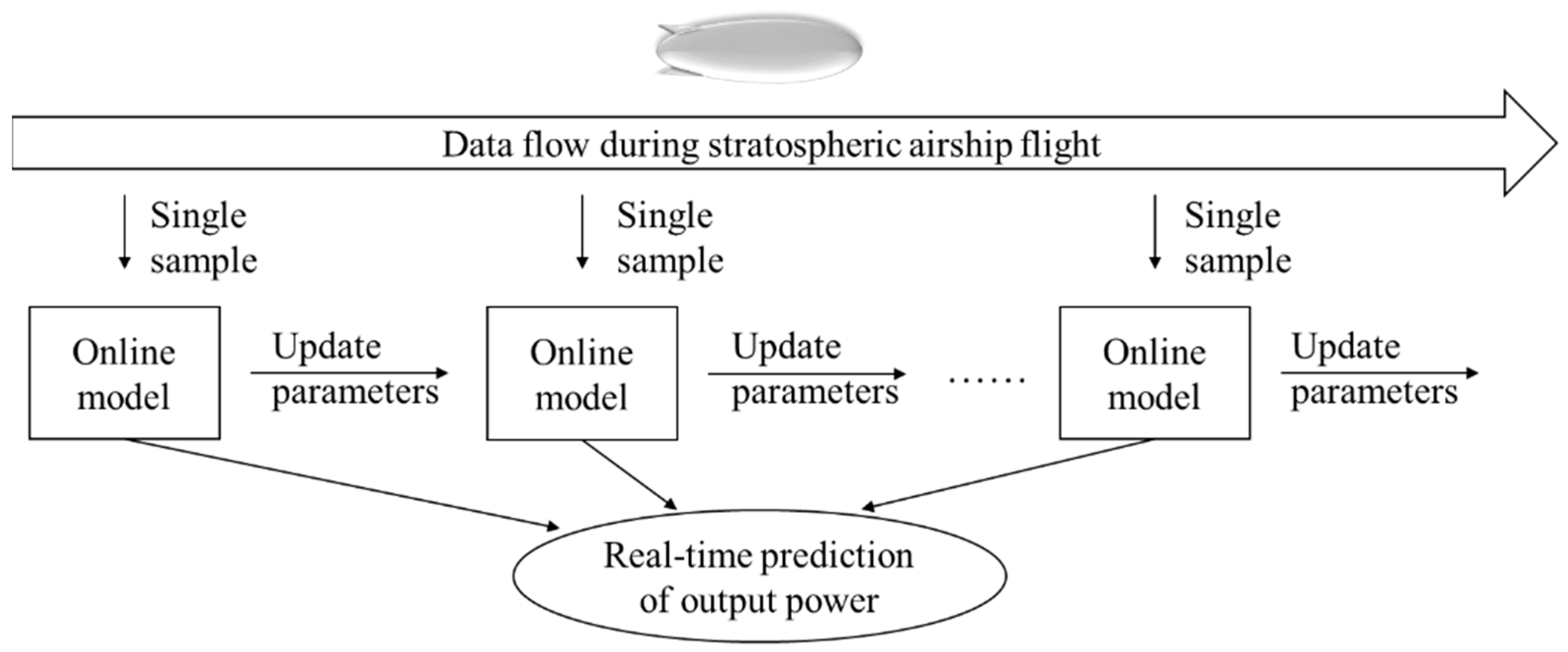
Parameter updating: Unlike offline learning models, online learning models use data streams for training. This means that only one set of samples will be sent to the training model at the same time. The model uses this sample for incremental learning instead of learning on the entire dataset. After the parameter is updated, the next set of samples is sent in. The sample collection and model training are synchronized, and each set of samples will be discarded after training and not stored in the memory. This significantly reduces the consumption of computing resources.

Figure 1 shows the online learning process of training a solar array output power prediction model using data streams during stratospheric airship flight.

3. Research Sample

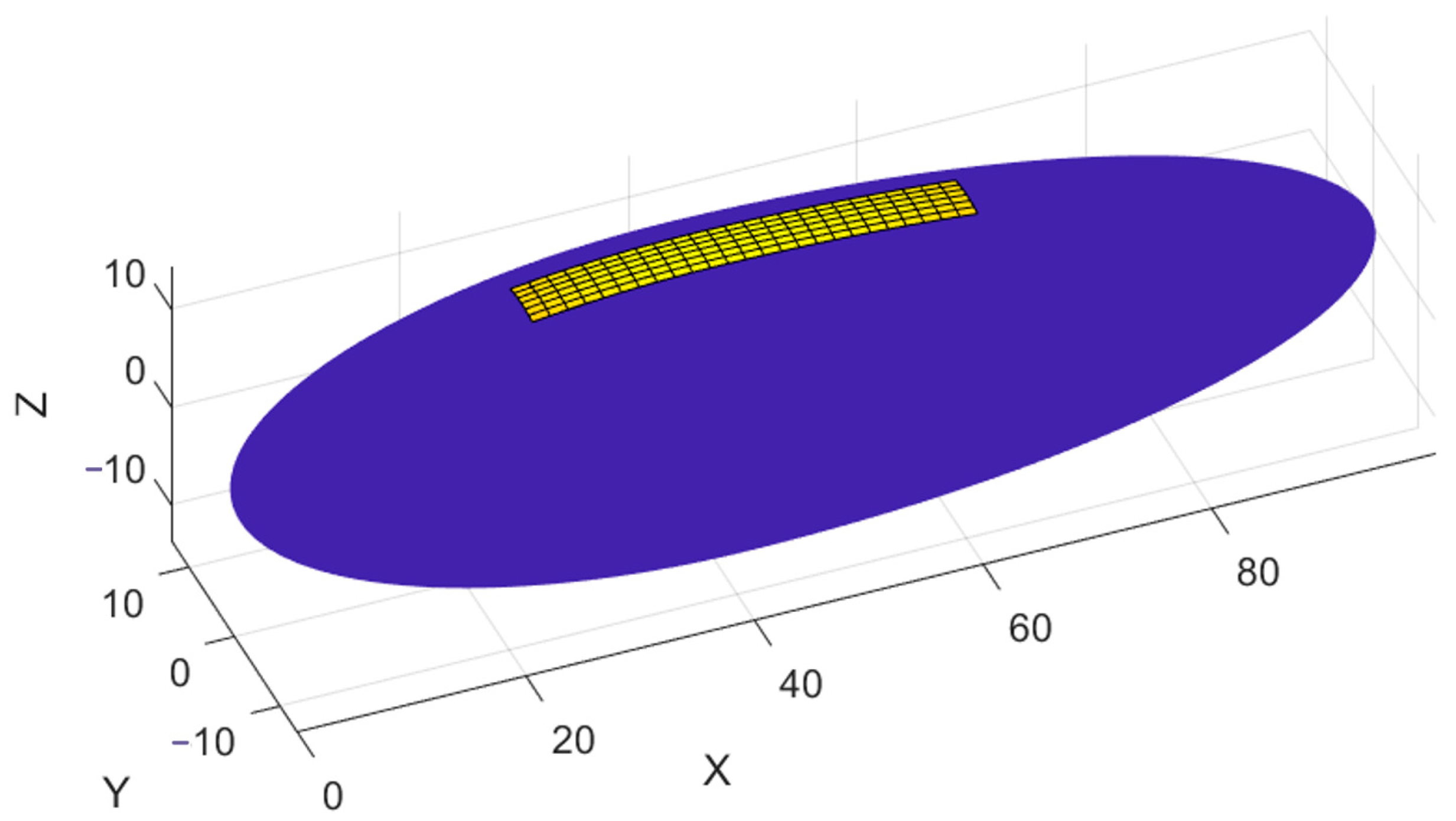
Due to the long flight test cycle and high cost, high-precision simulation models are used as research objects. As shown in Figure 2, the airship adopts the National Physics Laboratory (NPL) configuration, and the photovoltaic modules use SunPower’s E20_245 [29].

The specific parameters of the airship and array in the simulation model are shown in

Table 1. Design parameters of stratospheric airship.

Design Parameter	Value
Airship length (m)	100
Airship maximum diameter (m)	27.5
Airship volume (m3)	39,434
Solar array length (m)	39
Solar array width (m)	4.8
Photovoltaic module length (m)	1.558
Photovoltaic module width (m)	0.798
Module nominal power (W)	245

.

The output of the solar array is related to the received radiation intensity and temperature, and solar radiation intensity is the main influencing parameter. Radiation sensors are placed near the array to obtain radiation data. In addition, the solar panel array laid on the stratospheric airship has a large area. Due to the influence of the surface curvature of the airship, the positions of the photovoltaic modules on the airship are different, and the received radiation intensity is also different. Compared with uniform radiation, the total output power of the array will decrease, which is called mismatch loss [30]. Therefore, a single radiation sensor may not accurately reflect the overall radiation received by the array, and it is necessary to arrange multiple sensors to collect radiation data.

Assuming that the radiation intensity at the very top of the airship is obtained, the direct radiation intensity received by the radiation meter arranged on the surface of the airship can be calculated using the following formula:

$$I_i=I_h\cos {\theta }_i=I_h\frac{\overrightarrow{n_i}·\overrightarrow{n_s}}{\left|\overrightarrow{n_i}\right|\left|\overrightarrow{n_s}\right|}=I_h\left(x_i{x}_s+y_i{y}_s+z_i{z}_s\right)=I_h\left[x_i,y_i,z_i\right]\left[\begin{array}{l}{x}_s\\ y_s\\ z_s\end{array}\right]$$

(12)

where $I_i$ is the radiation intensity received by radiation sensor, $I_h$ is the radiation intensity at the flight height, $\overrightarrow{n_s}$ is the incident light vector, and $\overrightarrow{n_i}$ is the normal vector of radiation sensor.

The $I_h$ can be solved using three different positions of the radiometer.

$$\left[\begin{array}{l}{x}_s{I}_h\\ y_s{I}_h\\ z_s{I}_h\end{array}\right]={\left[\begin{array}{ccc}{x}_1& y_1& z_1\\ x_2& y_2& z_2\\ x_3& y_3& z_3\end{array}\right]}^{-1}\left[\begin{array}{l}{I}_1\\ I_2\\ I_3\end{array}\right]$$

(13)

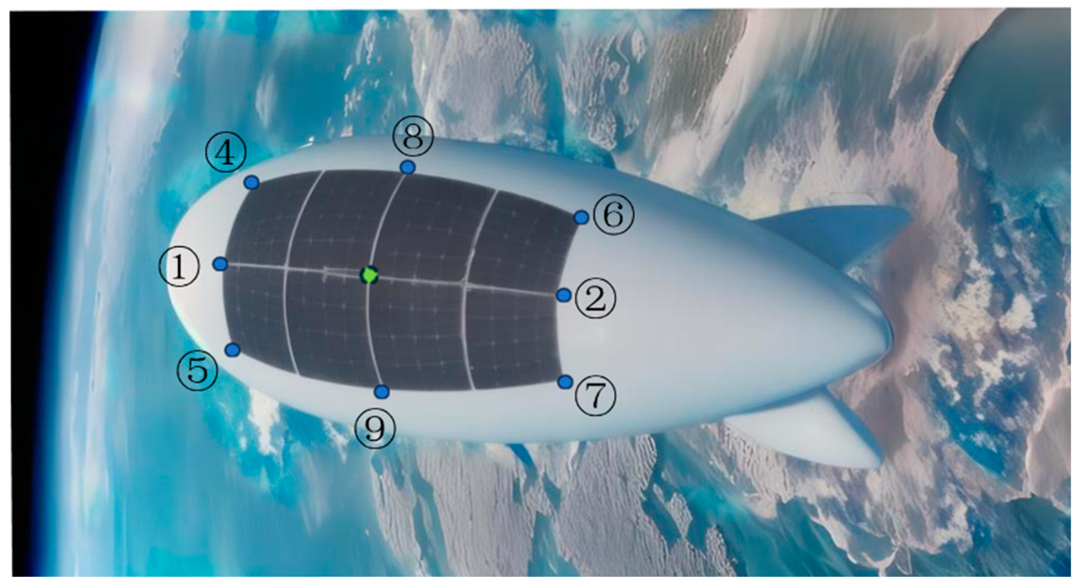
Figure 3 shows the location of the sensors as they are arranged on the airship (although the No. 3 irradiation meter in the middle is not actually used, a position is still reserved for it here). Eight irradiation meters are located around the perimeter of the solar array to reflect the intensity of irradiation at each photovoltaic module in the array without affecting the operation of the solar array.

During the prediction process, after the flight mission of the airship is given, the radiation meter index at any time can be calculated by the solar radiation model and the geometric model of the airship and then input into the online model to predict the output power.

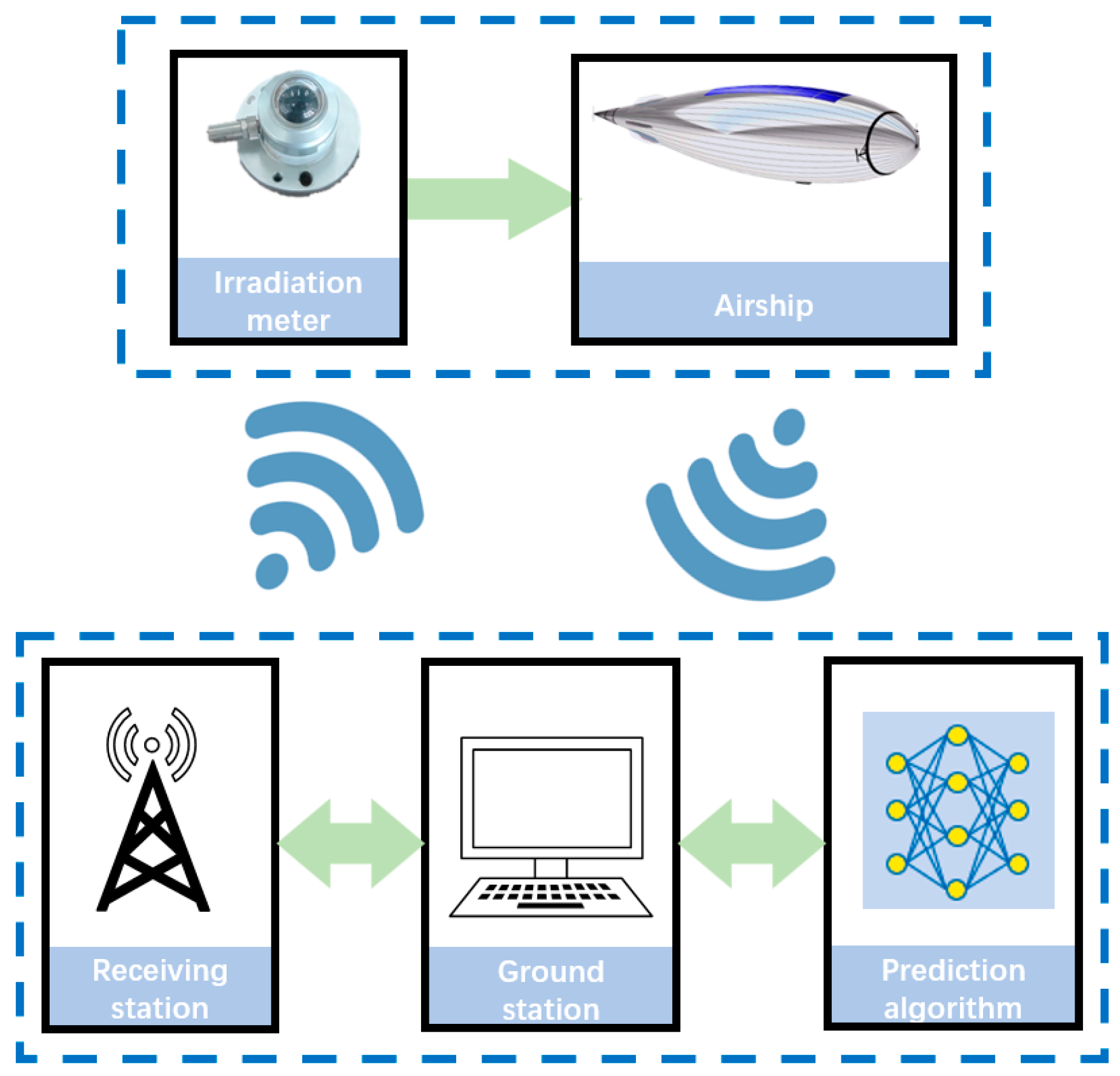
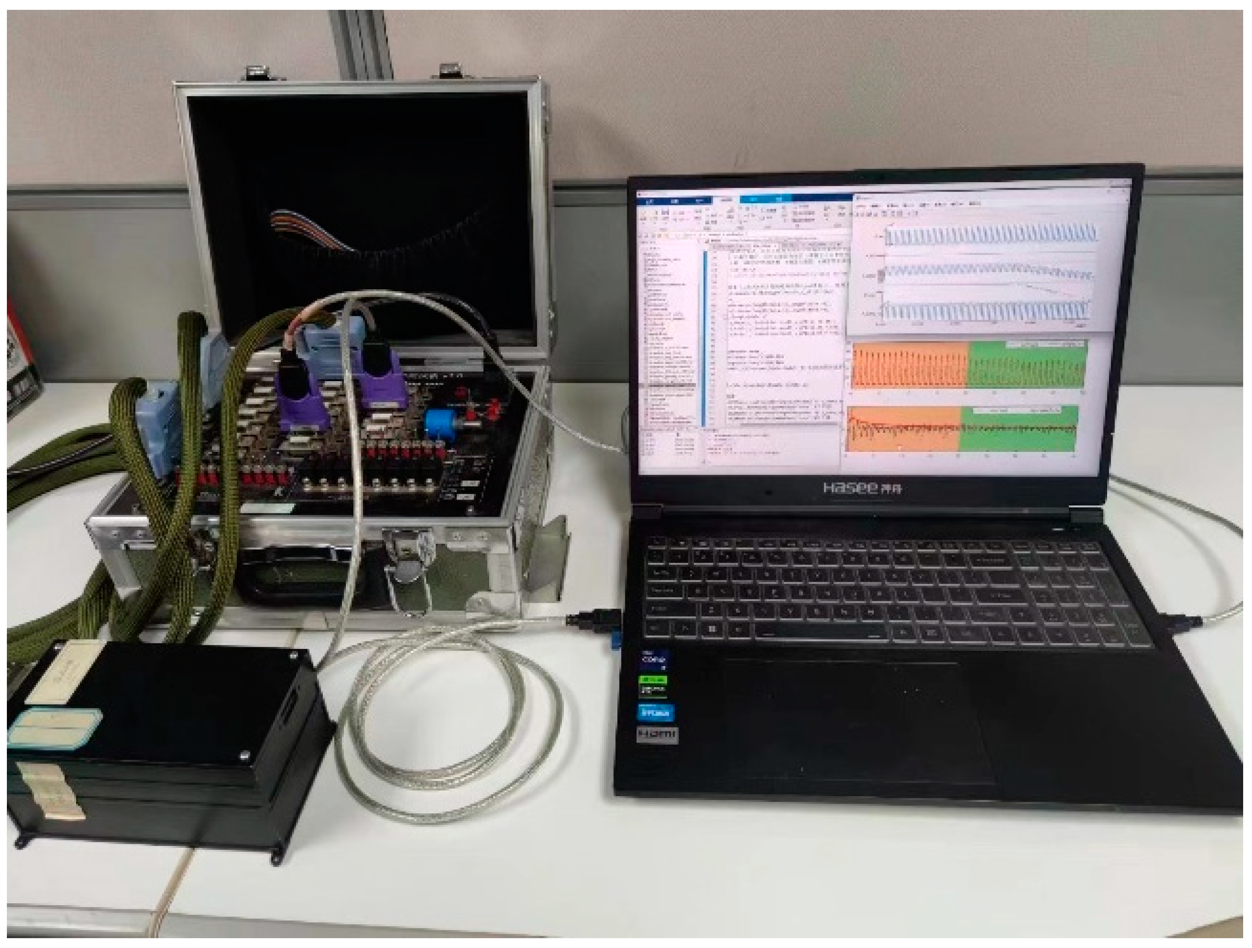
In order to facilitate a systematic analysis of the above design scheme, a ground physical principle verification system was constructed based on the correlation diagram in Figure 4 (which is based on future data acquisition, analysis, and transmission scenarios), as shown in Figure 5.

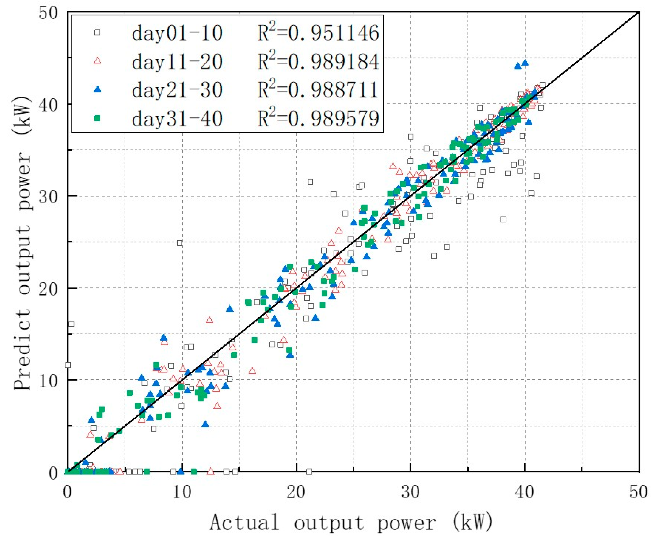
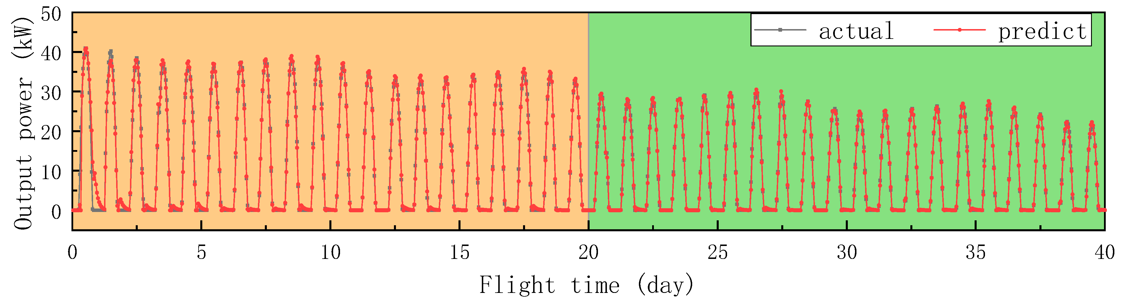
Assuming a flight mission for monitoring Australian wildfires, the airship will perform regional monitoring flight at a height of 20,000 m above Australia, with a flight radius of 900 km. The flight period is 40 days, from 31 January to 11 March. Samples are collected every hour, including sensor values and output power of solar array. To reflect the temporal characteristics and improve the prediction accuracy, in addition to using radiation values as input features, the output power and its first-order difference of the previous moment are also used. The performance indicator is evaluated using mean absolute error (MAE), which is consistent with the deviation of the actual output power in terms of order of magnitude.

$$MAE=\frac{1}{n}{\displaystyle \sum _{i=1}^n\left|\widehat{y_i}-y_i\right|}$$

(14)

4. Results and Discussion

4.1. Predictive Performance of Online Models

Figure 6 shows the array output power predicted by the online learning model trained using a single radiation count value. In the first 10 days of the flight, the online model had not learned all the features due to the small number of training samples, and the accuracy was low. After 20 days, the online model had obtained enough samples, and the accuracy was improved. As the flight continued, the online model prediction accuracy remained basically unchanged, and the training reached saturation. In addition, it can be seen that the points far from the diagonal are concentrated near the x-axis, which indicates that the sample points with actual output power are predicted by the online model as having no output. This error is mainly caused by the classifier. Using a better-performing classifier can further improve the model’s accuracy.

Table 2. Prediction accuracy during different flight period.

Flight Period (day)	MAE	Root Mean Square Error (RMSE)	Actual Mean Output Power (kW)	Percentage Error (%)
1–10	1.76	3.61	14.12	12.48
11–20	0.87	1.67	13.35	6.49
21–30	0.90	1.67	13.17	6.82
31–40	0.82	1.56	12.52	6.54
total	1.09	2.29	13.29	8.18

shows the specific prediction errors of the online model during the flights. After 20 days of flight data input into the training model, the prediction accuracy of the online model was reduced to half of its accuracy after 10 days and remained essentially unchanged for the remainder of the time. The final prediction percentage error over the entire flight period was 8.18%.

4.2. Effect of Irradiator Arrangement on Prediction Accuracy

Figure 7 shows the effect of different radiation meter placement methods on the prediction accuracy of the online learning model. From top to bottom, it represents the situation where 4 irradiation meters/3 irradiation meters/2 irradiation meters are placed around the solar array on the top of the stratospheric airship. So, it should be noted that the data displayed above the three graphs represent the actual corresponding irradiation meter numbers for the curve. For example, “4567” in the topmost graph represents the positions of the four irradiation meters, corresponding to the positions of irradiation meter 4, 5, 6, and 7 in Figure 3. The meanings represented by other numbers can be inferred according to the above rules.

From the trend of data changes in Figure 7, it can be seen that for all placement schemes, the prediction error was large and fluctuated in the first five days. As flight time increased, more samples were sent for training, and the prediction error of the model continued to decrease. After completing 40 days of flight, the predicted error-accumulated loss power was reduced to between 600 W and 800 W. In the radiation meter placement scheme, the more radiation meters, the lower the prediction error. When the same number of radiation meters are used, placing the radiation meters at the corners of the array instead of the midpoint of each side will result in lower prediction errors. When using four radiation meters, the lowest error, which was 0.64 kW, was obtained by placing them at the four corners of the array.

4.3. Online Prediction Considering Attenuation and Damage

Stratospheric airships fly at an altitude of about 20,000 m, where the air is thin and the air pressure is low. During the flight, due to the alternation of day and night, the temperature swing of the photovoltaic modules can be 100 °C, which may cause damage and affect the output power of the array. In addition, the encapsulation film will also age under sunlight, reducing its transmittance capability and thus affect the conversion efficiency of the photovoltaic modules. The solar cells in the photovoltaic modules may crack due to the influence of wind gusts, which will also significantly affect the output power [31].

Figure 8 and Figure 9 show the output power prediction results considering potential module attenuation and damage. Assuming that the conversion efficiency of the modules decreases by 1% after every day–night cycle, three adjacent modules in the solar array are damaged and stop working on the 20th day of the flight. Figure 8 shows the real output power and the predicted output power. Except for the first few days of the flight when the model had not yet fully learned, the predicted power is very close to the actual power for the rest of the time, and the predicted output is fully reflected the attenuation of the efficiency. Figure 9 shows that after the photovoltaic modules are damaged, the predicted error does not show significant fluctuations, and the online model quickly discovers the damage to the modules and adjusts the prediction results.

5. Conclusions

This paper proposes an online learning model for predicting the output power of a stratospheric airship solar array. The relevant parameters in the model can be continuously updated during the flight process, which can be used for the real-time prediction of the output power during continuous flight of the airship and can be used to guide autonomous flight. The model has the characteristics of low computational resource consumption and high accuracy, and the performance of the online model was verified by simulating a continuous flight process. The specific conclusions are as follows.

For a continuous flight of 40 days, the average prediction accuracy of the online model for output power can reach 92%. Indeed, the accuracy already meets the requirements by the 20th day. Increasing the number of radiometers can yield more illumination details for training the online model, thereby improving its accuracy. For the same number of radiometers, the accuracy is higher when they are arranged at the corners of the array than when they are arranged at the center of each side. The highest accuracy appears when four radiometers are, respectively, arranged at the four corners of the array, and the prediction accuracy is 95%. The proposed online learning model can also deal with the effect of potential modules attenuation or damage on the predicted output.