Article

Comparative Study of Soft In-Plane and Stiff In-Plane Tiltrotor Blade Aerodynamics in Conversion Flight, Using CFD-CSD Coupling Approach

National Key Laboratory of Rotorcraft Aeromechanics, Nanjing University of Aeronautics and Astronautics, Nanjing 210016, China
*
Author to whom correspondence should be addressed.
Aerospace 2024, 11(1), 77; https://doi.org/10.3390/aerospace11010077
Submission received: 31 August 2023 / Revised: 2 January 2024 / Accepted: 9 January 2024 / Published: 15 January 2024
(This article belongs to the Special Issue Applied Aeroelasticity and Fluid-Structure Interaction)

Abstract

:
Tiltrotors permit aircrafts to operate vertically with lift, yet convert to ordinary forward flight with thrust. The challenge is to design a tiltrotor blade yielding maximum lift and thrust that converts smoothly without losing integrity or efficiency. The two types of blades, soft in-plane and stiff in-plane—the designation depending on the value of the blade’s natural lag frequency—exhibit different structural responses under the same flight conditions, differently affecting the aerodynamics of the blades, especially in the complex aerodynamic environment of conversion flight where the aerodynamic differences are significant. This phase of flight is not deeply researched, nor is the analytical coupling method much used. To study the influence of blade type on aerodynamics during conversion, models suitable for the conversion flight simulation are established for the application of coupled computational fluid dynamics and computational structural dynamics (CFD-CSD) methods. Each method is implemented with well-accepted techniques (the Unsteady Reynolds-Averaged Navier–Stokes (URANS) equations, the Reverse Overset Assembly Technique (ROAT), and the Timoshenko beam model. To improve the solving efficiency, a loose coupling strategy is used in constructing the two-way coupled model. The XV-15 tiltrotor is used for verification. The aeroelastic simulation of soft in-plane and stiff in-plane blades in conversion flight indicates an impactful role on the modal shapes, with a significant difference in the third flap modal shapes for the XV-15 rotor. However, the effect on aerodynamic performance is relatively small. In the first half of the flight conversion, the thrust of stiff in-plane blades is larger than that of soft in-plane blades, but in the last half, the influence of structural characteristics on aerodynamic performance is negligible and the thrust of the blades tends to be equal.

1. Introduction

Conversion flight is the unique flight mode of the tiltrotor, and its unsteady aerodynamic environment accentuates the blade aeroelasticity problem. After taking off and before landing, the pylon is tilted to transform between the aircraft flight mode and the helicopter flight mode. The incoming flow and the aerodynamic environment of the rotor blades change markedly, complicating the structural deformation and strongly affecting the aerodynamics of the blades. Former researchers, from the viewpoints of aerodynamics [1,2,3] and structural dynamics [4,5,6,7], simulated and analyzed conversion flight, demonstrating the relationship between tilt angle and the unsteady characteristics of the aerodynamic environment and the problem of aeroelastic stability that occurs in conversion flight. However, the influence of blade deformation on the aerodynamic characteristics of conversion flight is not deeply researched, and the coupling method has rarely been used in such investigations.
The aeroelastic characteristics of rotor blades are directly related to their structural characteristics. Tiltrotor blades are of two structural types: soft in-plane blades and stiff in-plane blades, designated according to the first-order natural lag frequency. Because the two blade types have different structural characteristics, they produce different structural deformations in the same aerodynamic environment [3,8,9]. Both blade types have advantages and disadvantages, and both are used in engineering design. Using stiff in-plane blades helps avoid the problems of ground resonance and air resonance; using soft in-plane blades can improve the handling quality. The present work uses structural dynamic modeling of soft in-plane and stiff in-plane blades to obtain their performance in conversion flight. The results verify and quantify, as functions of tilt angle, the effects on sectional normal force and rotor thrust induced by the different structural characteristics of the two blade types, allowing for the evaluation of the rotor performance in each case.
Previous researchers have studied the structural dynamic characteristics of tiltrotor blades in different flight conditions, but the aerodynamic models used were relatively simple. Corle et al. [10] studied the time domain dynamic response of tiltrotor blades with different inflow models. Krstic et al. [11] studied the stall flutter limit problem to solve the longitudinal force equilibrium of a helicopter. Masarati et al. [12] utilized a reduced order model to calculate aerodynamic forces. Most commonly, a wake model is used to generate the aerodynamic forces necessary for structural dynamic analysis [7,13,14]. These methods cannot couple the aerodynamic analysis and structural dynamic analysis to calculate the aerodynamic result, including the consideration of blade elastic deformation. The present work uses the computational fluid dynamic (CFD) method to simulate the flow field. The blade elastic deformation is simulated as the surface mesh movement with the reverse overset assembly technique [15] and mesh deformation. Hence, the two-way coupling of aerodynamic analysis and structural dynamic analysis is accomplished in the present work.
The computational fluid dynamics–computational structural dynamics (CFD-CSD) coupling approach is used in many studies to simulate the influence of structural deformation on rotor aerodynamic performance [9,16,17]. Lim [18] coupled OVERFLOW2 (CFD solver) and CAMRAD II (for CSD solving) to research the structural mechanism and optimize the blade performance. Previous research using the CFD-CSD coupling approach primarily focused on the simulation of the helicopter rotor, but the method has not been significantly applied in research on tiltrotor blades. A loose coupling strategy is used in the present work to couple the CFD and CSD models. The CFD analysis is based on the Unsteady Reynolds-Averaged Navier–Stokes (URANS) equations and the CSD analysis is constructed based on the Timoshenko beam model. The coupling method was used in a previous study [19] for the simulation of tiltrotor flow field during shipboard take-off and landing. By analyzing the results of soft in-plane and stiff in-plane tiltrotor blades in conversion flight, this study found that the influence of the difference in the structural characteristics of the blades on the aerodynamic force is quite different in the first and last halves of the tilting action, being more significant in the first half than in the last half. However, in the whole range of action in flight conversion, the thrust and normal force of the section near the blade tip of the stiff in-plane blade are larger than those of the soft in-plane blade.

2. Numerical Simulation Method

2.1. The Geometry, Structure, and Grid

In the present work, the advanced technology blades (ATB) rotor of the XV-15 tiltrotor [20] are used as the model blade. The XV-15 tiltrotor has three blades in each rotor. The radius of the rotor is R = 3.81 m, and its solidity is 0.103. The blade has nonlinear torsion of −47° and root at 0.1 R. The average chord length is 0.411 m, and the shape of the blade tip is square. The blade shape and airfoil distribution are shown in Figure 1 [21]. Figure 2 shows the schematic diagram of the tilt angle. The rotor is placed on the front of pylon (the left and top on Figure 2). The aircraft flight mode (red in the figure) is defined at a tilt angle of 0°, and the helicopter flight mode (blue in the figure) is defined at a tilt angle of 90°. In this study, the rotational speed was 59.17 rad/s, and the free flow velocity was 15 m/s, with Reynolds number Re = 4.62 × 10⁵.
The grid system includes blade and wing grids with C-H topology, as well as Cartesian background grids. Among them, the cell number of the single blade grid is 1.875 million, the wing grid is 1.849 million, and the first layer (near the entity object surface) height is 2.15 × 10⁵ m, with a corresponding y+ value of 1.0. The background grid contains a fine-mesh region that surrounds the rotor and wing. At different tilt angles studied in this paper, the cell number of mesh in the fine-mesh region ranges from 7.77 million to 8.642 million, and the cell number of the coarse-mesh region is 4.506 million. We use wall boundaries to represent blade and wing entities and set the outer surface of the background mesh as a pressure far field. The assembly between multiple grid blocks is implemented by the overset method with interpolation boundaries among the assembled grid blocks. The ROAT proposed by the authors in previous research [15] is used for overset mesh interpolation to avoid the problem of orphan points in the overset mesh system and to improve the robustness of deformable mesh. The overset mesh system used in the present work is shown in Figure 3. The research of Potsdam et al. [22] indicated that the fountain flow over the aircraft is calculated differently in the simulations modeled by a full-span tiltrotor and a semi-span tiltrotor using the symmetrical boundary at the center of the aircraft. The present work uses full-span tiltrotor blade modeling to better simulate the flow field of the tiltrotor blade for a more accurate result.

2.2. The CFD Method

The CFD analysis in this study takes the RANS equations [23] as governing equations to solve the flow field in the fluid domain:
t V W d V + V F c n d S V F V n d S = 0
where:
W = ρ         ρ u         ρ v         ρ w         ρ E T
In the above equation, W represents the five conservative variables of three equations; F C and F V are the vectors of the inviscid and viscous flux, including the inner effect in the fluid domain. p, ρ, and E represent unit pressure, density, and energy, respectively. u, v, and w are the velocity vector components of the cell unit. n represents the velocity flux in the normal direction of the control surface.
The CFD solver is developed using C++ with a cell-centered store scheme. It supports the central or ROE spatial discretization, the explicit Runge–Kutta (RK) [24], and the implicit lower–upper symmetric Gauss–Seidel (LUSGS) [25] time discretization scheme, and the turbulence model can be set as an inviscid model with artificial viscosity and the Spalart–Allmaras (SA) model. The dual-step precise time integration method [26] is introduced for unsteady motion cases, which discretizes one rotor circle into several real-time steps and sets multiple pseudo-time steps on each real-time step, forming the URANS method. In the analysis of this article, the blade rotation is divided into 720 steps per turn. The solver can set independent spatial and temporal discretization formats and turbulence models for different mesh blocks. And it has good parallel and GPU acceleration performance. In addition, to achieve deformation simulation, the arbitrary Lagrangian–Eulerian (ALE) method [27] is used to convert the deformation into a virtual additional motion flux.
The flow field is divided into two parts: one is close to the body surface, and the other one is the peripheral fluid region. The peripheral region consists of a background mesh (including fine-mesh and coarse-mesh regions), the central scheme is used for spatial discretization, and the RK scheme is used for time discretization. In contrast, the near-body region uses the Roe scheme with the LUSGS scheme and the SA turbulence model. The SA turbulence model is widely used in rotor flow field simulation and also meets the needs of CFD/CSD coupling simulation. For example, Smith used it in the CFD/CSD coupling simulation of Hart II, which shows good accuracy [28]. In addition, the interaction of the rotor and wing is considered via overset interpolation in the present simulation.

2.3. The CSD Method

The CSD solver uses the Timoshenko beam model [8] to calculate the flap, lead–lag, and torsion displacements corresponding to the air load calculated by the CFD solver. Because for actual composite rotor blades, their cross-sections exhibit complex shear deformation and nonclassical effects such as elastic coupling caused by material anisotropy, the bendwise coupling is also included in the simulation.
The blade structure model comprises a two-dimensional linear section analysis and one-dimensional nonlinear beam analysis, as shown in Figure 4. The surface grid points are distributed in the cross-sections. This scheme balances computational accuracy and efficiency; the principle can be found in reference [29]. This differs from the method of calculating wing deformation using computational finite elements with structural mesh [30].
In this study, the blade is discretized into 50 segments along the spanwise direction, and the forces on the end faces of each segment can be obtained by postprocessing the flow field pressure of the grid faces between the segments. At the same time, the endpoint’s cross-section also serves as the deformation control cross-section. The detailed coupling process will be explained in the next section.
The blade beam model established by the Timoshenko beam has 20 degrees of freedom, including 4 degrees at the middle node of the element and 8 degrees at the two end nodes. It describes the displacement v i and w i and rotation angles v i , x and w i , x in the flap and lag directions, torsional displacement ϕ i , tensile displacement u i , and the shear degrees of freedom γ x η i and γ x ζ i . The schematic diagram is shown in Figure 5. So, the displacement composition at any point in the section can be decomposed into two parts: caused by rigid body motion and caused by section warping. The detailed principle can be found in references [31,32,33].
This model has high-order degrees of freedom and allows for free deformation at intermediate positions, making it suitable for CSD calculation of rotor blade deformation,, and for free deformation in the middle position, which can avoid the lack of shear degree and improve the accuracy of solving elastic coupling problems caused by shear deformation and the elastic anisotropy of the blade [8,34]. Therefore, compared to the Euler Bernoulli beam, it has a better ability to simulate the deformation of composite blades such as helicopters and tilt rotors [35].
For the displacement of any point on the blade, the following interpolation formula can be used for Timoshenko beams:
v w f u γ ¯ x η γ ¯ x ζ = D i a g Φ v T Φ w T Φ f T Φ u T Φ η T Φ ζ T V W f U Γ x η Γ x ζ
In Equation (3), Φ v to Φ ζ are spatial interpolation functions only related to coordinates, while the term in the right vector is a time variable. By using the finite element method to assemble all elements, the mass, damping, and stiffness matrices of the overall structure and vector forces can be obtained. Finally, a second-order linear ordinary differential equation describing the dynamic characteristics of the blade can be obtained as follows:
M q ¨ + C q ˙ + K q = Q
where M represents the mass matrix, C is determined by material parameters, K is the stiffness matrix, and Q is the external force vector.
In this study, the structural parameters were derived from the basic measurement data of XV-15 described in reference [36] and calculated proportionally through geometric anisotropy distribution. The CSD solver will output displacement and rotational deformation information at each segment endpoint of the blade at the azimuth corresponding to the CFD solution time step.

2.4. The CFD-CSD Coupling Method

This paper adopts a loose coupling strategy [18,20,37] to achieve the coupling calculation between CFD and CSD, and the established coupling process is shown in Figure 6. It is mainly divided into four steps.
(1) Flow field simulation. After motion and overset assembling the mesh blocks, the CFD solver calculates the flow field of the rotor at each azimuth of the revolution and obtains the corresponding surface pressure data of the blade at each azimuth angle.
(2) Convert the surface pressure information into the input of the CSD solver. Calculate the forces and moments at different azimuth angles and spanwise positions during a rotation. This process first obtains the force on the surface by multiplying the area and pressure of the surface element. Then, it sums up the force on the surface element and the moment to the corresponding section’s 1/4 chord line contained in the segment.
(3) Calculation of deformation information of blade. Based on the Timoshenko beam model, the CSD solver calculates the translation and rotation information of each segment endpoint on the blade at each azimuth and outputs it.
(4) Obtain deformed mesh via deformation information. Calculate each node point’s coordinates for each azimuth after deformation using the endpoints’ displacement and rotation information. The grid nodes located in the middle of the segment can be obtained through linear interpolation of displacement and rotation at the segment of two ends. As shown in Figure 7, the position of the deformed grid points is determined based on the deformation of the two segment endpoint’s cross-sections where they are located. In the figure, grid point P corresponds to cross-section S P (with spanwise L P ), located between cross-sections S 1 and S 2 (with spanwise L 1 and L 2 ). It is projected onto the original cross-sections S 1 and S 2 as points P S 1 _ o r i g and P S 2 _ o r i g , respectively. As the cross-sections S 1 and S 2 deform, they become P S 1 _ n e w and P S 2 _ n e w , and the position after deformation is P n e w = ( L P L 1 ) / ( L 2 L 1 ) × ( P S 2 _ n e w P S 1 _ n e w ) + P S 1 _ n e w . Specifically, the points located inside the blade root or outside the tip are determined by the segment endpoint’s cross-section of the blade root or tip, respectively. Also, the relationship between them and the cross-section of the root or tip remains unchanged after the deformation of the blade.
Finally, a complete CFD/CSD solution can be formed by looping the above four steps until the simulation converges. In the above process, steps (2) and (4) can be integrated as the preprocessing of the grid and postprocessing of the flow field in the CFD solver. The information transfer between the two programs is completed using a Python-based communication program, which only transmits load and deformation information without any changes. Due to the periodicity of the rotor flow field, during the loose coupling process, information on various azimuth angles and cross-sections within a turn can be transmitted via data exchange once. That is, a coupling process can generate forces for calculating deformation at all azimuth angles of a turn and deformation information at all azimuth angles.
It should also be noted that to accelerate the simulation process, the initial mesh deformation in the simulation can be obtained from experimental data directly or calculated through the estimated load from blade element theory or lift surface theory, etc. At the same time, to provide stability for the coupling simulation, the CFD/CSD coupling simulation will be carried out only after the flow field exhibits a relatively stable period. It was a CFD-only simulation before this and usually needs 4 turns in this study. The calculation will continue until convergence, which generally requires an additional 4 turns of CFD/CSD coupled simulation.

3. Verification of Simulation Method

This section focuses on the verification of CSD and CFD-CSD coupling. The author team has mastered mature rotor CFD-solving methods in previous research and developed an in-house solver, RADAS (rotorcraft aerodynamics and aeroacoustics solver) [38]; so, CFD verification is omitted here. Detailed verification can also be found in the authors’ previous research [39,40,41].

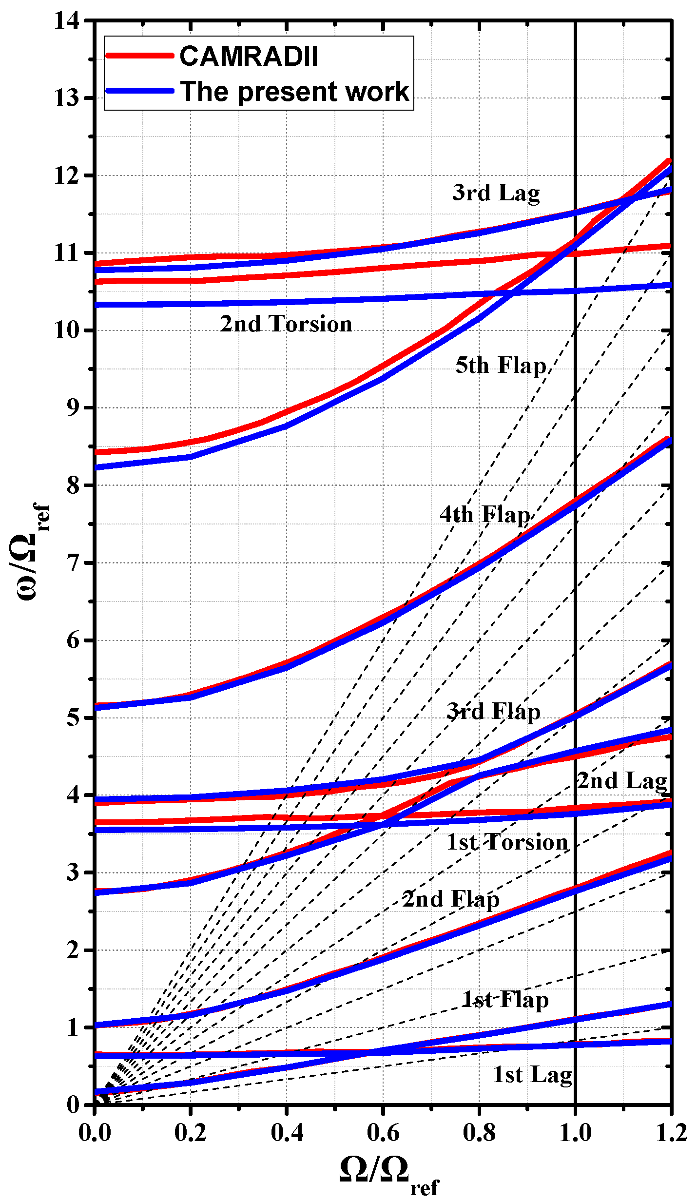
3.1. Verification of Structural Characteristic Calculation

The structural characteristics validation calculations were conducted on the Bo-105 blade. Figure 8 compares the calculated values of the blade resonance diagram in this article and the calculated values of CAMRAD II [28]. It can be seen that the resonance diagram calculated in this article is in good agreement with the calculated values of CAMRAD II, and the characteristic is that it completely coincides with the curve of CAMRAD II in the low-frequency region that has a significant impact on the inherent characteristics of the blade. Figure 9 compares the calculated vibration mode curve of this article with the computed values of the AFDD-1 project [28], and it can be seen that the CSD method in this article can effectively predict the blade vibration mode curve. The slight differences may be due to differences in structural segment numbers compared to the references.

3.2. Verification of the CFD-CSD Coupling Method

The forward flight test state of the Hart-II rotor [36] is used to verify the effectiveness of the CFD/CSD aeroelastic coupling method established in this article. The rotor of this model is composed of four hinge-free Bo-105 blades with a radius of 2 m and a chord length of 0.121 m. The airfoil uses NACA13012, with a linear twist of −8° and a rotor axis rake angle 2.5°. This paper calculates the experimental state with a forward ratio of 0.151 and a blade tip Mach number of 0.639, including higher order control harmonics. Figure 10 compares the calculated value of the 0.87R section normal force coefficient obtained after 10 cycles of aeroelastic coupling calculations and the experimental value [28], and both the calculated and experimental values have been averaged. Compared with a previous study by Liu et al., which only focused on significant trends, the results of the present coupling method are more consistent with the experimental values. Still, on the latter side, ψ = 0°. The calculated value at around 0° is slightly higher, possibly due to the trailing blade’s severe stall. The CFD solver needs to consider both the reflux and low-pressure regions, resulting in a deviation between the calculated results and the experimental values.

3.3. Verification of Grid Independence

We built three grid systems to verify the independence of the grid. The grid element numbers of coarse, baseline, and fine systems are shown in Table 1. The normal force coefficients of the three systems are compared, as illustrated in Figure 11. The results verify the independence of the grid and baseline grid systems used in this study, and no obvious difference was observed between all three meshes. Moreover, considering that the calculation of blade CSD mainly focuses on the in-plane load, even a coarse mesh can ensure good simulation results. In similar rotor CFD/CSD simulations by Liu et al. [42], usable results were also obtained on the 5 million grid.

4. Discussion and Results

4.1. Analysis of Structural Characteristics

The present work models and analyzes soft in-plane and stiff in-plane blades; of particular interest are the variations in behavior as functions of the tilt angle. The detailed data defining structure are shown in Table 2, where EA, EIηη, EIζζ, and GJ represent axial stiffness, lagwise bending stiffness, flapwise bending stiffness, and torsional stiffness, respectively; ωv is the ratio of first-order natural lag frequency to the rotational speed of the rotor. For the soft in-plane blade, ωv is less than 1.0, while for the stiff in-plane blade, it is larger than 1.0.
Figure 12 compares the frequency diagrams of soft in-plane and stiff in-plane blades. Since the impact of lower order frequency vibration is larger than that of higher order, only the lowest modal frequencies are shown as a function of rotational speed. The comparison in the figure reveals that due to the different flapwise bending stiffness of the soft in-plane and stiff in-plane blades, the flap frequency has changed greatly; however, due to the existence of the flap–lag coupling vibration, only the bending stiffness in the flapwise direction is changed, and the lagwise frequency curve also changes to a small extent. Figure 13 shows the modal shape diagrams of the third and fourth orders of lead–lag modes and the second and third orders of flap modes. From the comparison of the soft in-plane and the stiff in-plane blades, the node positions of the modes do not change greatly, but the difference in the structural characteristics of the blade leads to a large change in the amplitude of the modal shape. In particular, the extreme value point of the third flap modal shape is around 0.4R, whereas the figure of the soft in-plane blade is about 47% of that of the stiff in-plane blade.

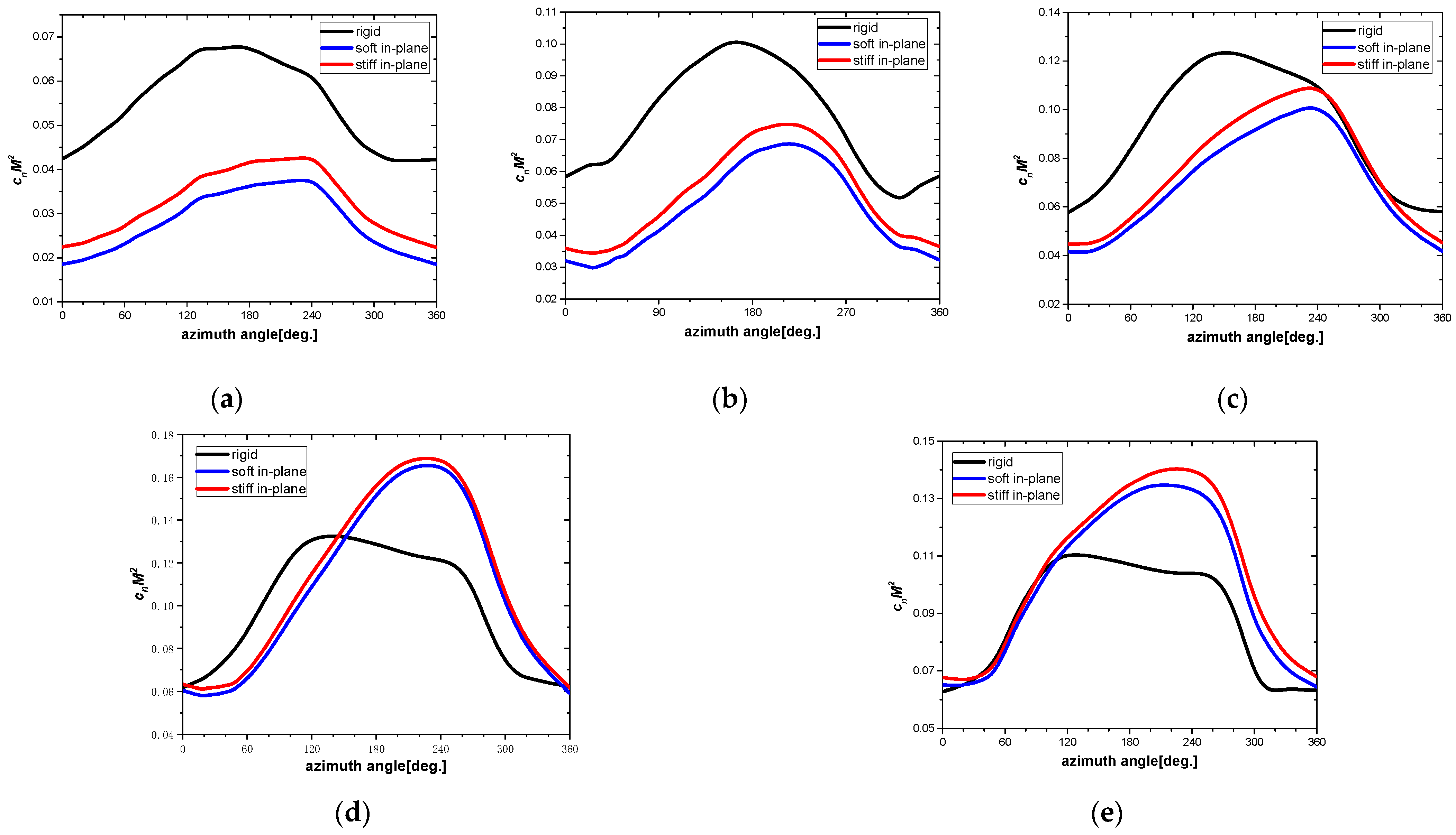
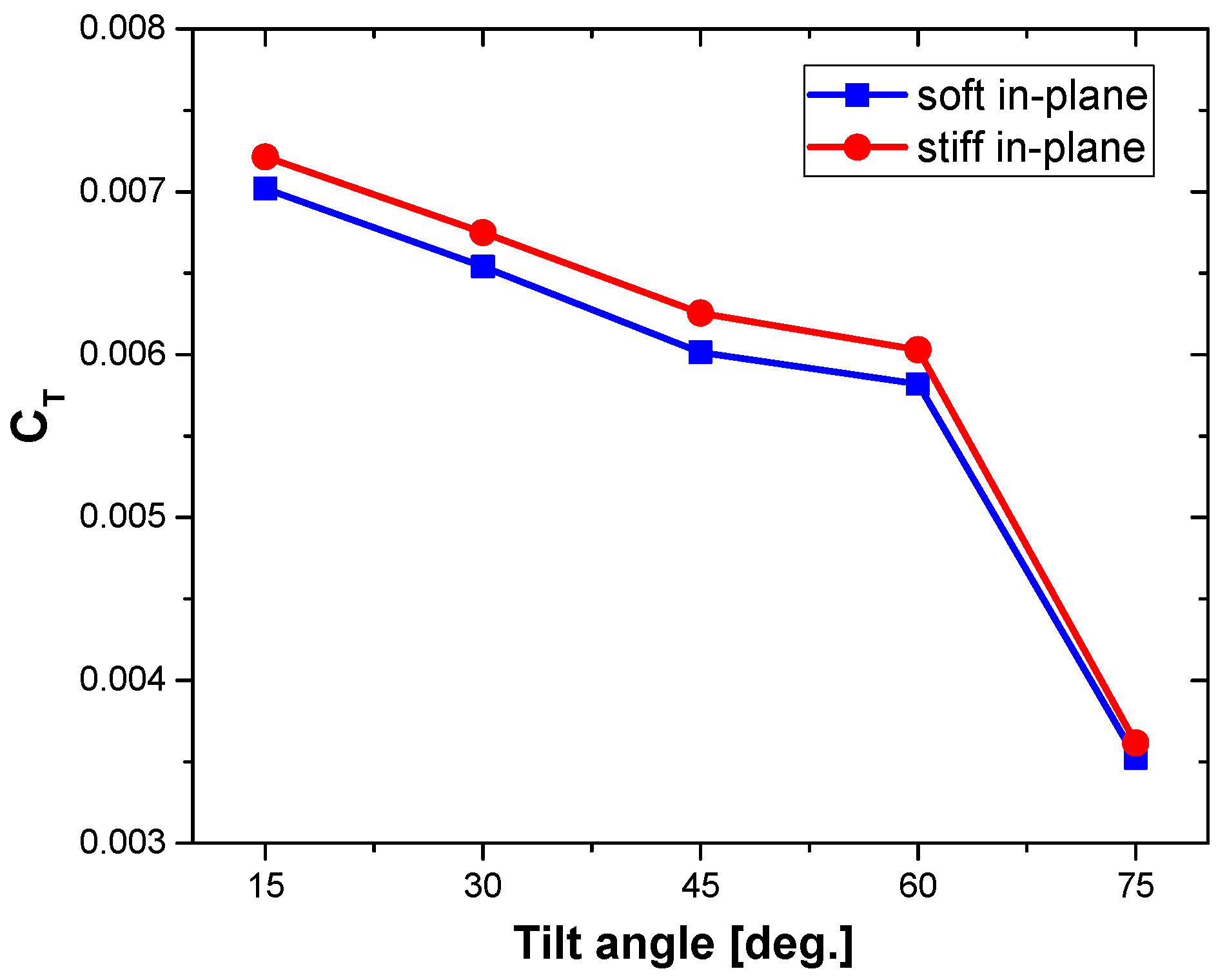
4.2. Influence of Tilt Angle on Aerodynamic Characteristics of Soft In-Plane and Stiff In-Plane Blades

In order to study the influence of the tilt angle on the normal force of the soft in-plane and stiff in-plane blades, the flow field of the two blades is calculated at various tilt angles from 15° to 75° (with incoming still flow 15 m/s), and normal forces on spanwise sections from 0.5R to 0.95R were compared. The difference in the normal force coefficient and the normal force coefficient difference divided by the mean value are defined as follows:
Δ c n M 2 = c n M 2 s t i f f c n M 2 s o f t
Δ c n M 2 c n M 2 ¯ = c n M 2 s t i f f c n M 2 s o f t ( c n M 2 s t i f f + c n M 2 s o f t ) / 2
Figure 14a shows the variation in the difference in the normal force coefficient of soft in-plane and stiff in-plane blades on spanwise positions as a function of the tilt angle, and Figure 14b shows the relative difference which is the ratio of the normal force coefficient to the mean value of soft in-plane and stiff in-plane blades to analyze the influence of structural characteristics on the variation in thrust around a revolution. The results show that the difference in the normal force coefficient is larger near the blade tip, while at section 0.5R, closer to the blade root, the difference between the soft in-plane and stiff in-plane blades’ normal force coefficient is small. At a tilt angle of 75°, the relative difference is only 0.077%.
Since the sectional normal force of the rotor blade increases first and then decreases along the spanwise direction, the main position for providing thrust is about 0.75R, near the tip of the blade, where the effect of torque is greater than that at the root of the blade. The thrust can be regarded as a force distributed along the span, and the deformation is superimposed from the root to the tip, resulting in a greater impact on the aerodynamics due to the different elastic deformation at the blade tip. However, on the sections from 0.85R to 0.95R closest to the tip of the blade, the difference curves of the normal force almost overlap. Due to the large geometric pitch angle of the blade tip section, it is in a state of stall at a large angle of attack. The change in the angle of attack caused by the deformation has a limited impact on the aerodynamic environment of the section, so the aerodynamic difference is no longer sensitive to the spanwise position. On section 0.95R, the curve moves downwards, and the difference between the normal forces of the two blades is less than 0.9R at each tilt angle.
The difference in the normal force coefficients at different spanwise sections maintains the same trend: from 15° to 75°, it first increases slowly and then decreases, and the inflection point is at a tilt angle of 45°. The upward trend is more obvious near the tip of the blade, while on the spanwise sections near the root of the blade, it is basically unchanged at tilt angle of 15°–45°. From the relative difference curve in Figure 14b, it can be seen that the change in the normal force coefficient caused by the different blade characteristics relative to thrust variation also increases first and then decreases with the change in the pitch angle. This downward trend becomes more and more severe from 0.5R to the tip sections along the span, indicating that the change in the soft in-plane and stiff in-plane structural characteristics has a greater impact on the aerodynamic force on the sections closer to blade tip. In summary, when the rotor tilts from the aircraft flight mode to the helicopter flight mode, the change in the sectional normal tension caused by the change in the structural characteristics in the first half of tilting motion is not sensitive to the tilt angle. However, in the last half of the motion, the increase in the tilt angle will significantly reduce the normal force difference of each section, and the aerodynamic differences between blades with different structural characteristics are no longer obvious.
Figure 15 and Figure 16 compare the curves of the normal force coefficient with the azimuth angle of the soft in-plane blade, stiff in-plane blade, and rigid blade on sections of 0.75R and 0.95R, respectively, at the five different tilt angles. The rigid blade is the result calculated by the CFD method without considering the elastic deformation. The figure shows that at small tilt angles (15°–30°), the elastic blade always causes the normal force to drop, and the normal force of the rigid blade is always greater than that of the blades with elastic deformation. At a 45° tilt angle, the data of the three curves around the 270° azimuth angle are very close, and the normal force of the stiff in-plane blade is slightly larger than that of the rigid blade. But on the forward side of the rotor, the normal force of the rigid blade is still significantly greater than that of the elastic blades. In contrast, the normal force of the elastic blades on the retreating side at a tilt angle of 60°–75° is significantly greater than that of the rigid blade. The normal force coefficient curves of the rigid blade and the elastic blades have no intersection point at a small angle of tilt, and the intersection point starts to appear on the retreating side at tilt angle of 45° and moves to the forward side with the increase in the tilt angle. At a tilt angle of 75°, the intersection point is about an azimuth of 90°. The main difference between the blade tip (0.95R) and 0.75R is that the normal force change trend of the rigid blade and the elastic blades is no longer the same under the tilt angle of 45°–75°. In the second–third turn (azimuth angle of 120°–240°), the rigid blade normal force curve has a slowly varying plateau, while the elastic blade results have no significant plateau.
Figure 17 shows the variation trend of the soft in-plane and stiff in-plane blades’ thrust coefficients with pitch angle. In the conversion flight, the thrust of the stiff in-plane blade is always greater than that of the soft in-plane blade. The difference between the thrust of the two blades at a tilt angle of 15°–60° remains basically unchanged. At 60°–75°, there is a rapid drop in thrust, and the thrust of the soft in-plane and stiff in-plane blades at a tilt angle of 75° is basically equal, with a difference of about 2.5%.
Figure 18 shows the distribution of the difference in the normal force coefficient of the soft in-plane and stiff in-plane blades at various positions of the rotor disc. The incoming flow is from directly below (180° azimuth) to directly above (0° azimuth). The figure shows that when the tilt angle is 15°, the part with a large difference in normal force is roughly distributed in the ring area of 0.7R–1.0R. As the tilt angle increases to 60°, the difference between the two blades around the 180° azimuth becomes more and more prominent. At a tilt angle of 75°, the normal forces of the soft in-plane and stiff in-plane blades tend to be equal. The difference in normal force at each position of the rotor disc is small, which is consistent with the change in the tension coefficient in Figure 17.
Figure 19 and Figure 20 show the slices of contour of the vorticity under the Q criterion calculated in the present work. Figure 19 is the bottom view at a tilt angle of 15°, and Figure 20 is the side view at a tilt angle of 60°. All of the slices pass through the rotor axis. The figures show that the method used in the present work can predict the structure of the vortex well, and the changes in the wake vortex after being disturbed by the wing are also clearly captured. A comparison of the vorticity contours of the soft in-plane blade and the stiff in-plane blade shows that the vortex structures of the two are basically the same, and the change in the blade structural characteristics will not affect the wake vortex structure.

5. Conclusions

The coupled CFD-CSD analysis based on the RANS equations and the Timoshenko beam model was used to simulate tiltrotor blades in conversion flight with soft in-plane and stiff in-plane blades to analyze the influence of structural characteristics on tiltrotor blade aerodynamic performance. The normal force coefficient, rotor air load, and the structure of the wake were compared. The following conclusions were obtained:
(1) The influence of structural characteristics with soft in-plane and stiff in-plane blades on the normal force is greater at the blade tip than at the blade root, but on the 0.85R–0.95R sections near the blade tip, the difference between the normal forces of soft in-plane and stiff in-plane blades no longer varies with the change in sectional radius. This is due to the large geometric pitch angle at the tip of the blade, which has been in a state of stall at large angle of attack.
(2) When the tiltrotor converts from the airplane flight mode to the helicopter flight mode, the normal force difference in the soft in-plane and stiff in-plane blades in the first half of the tilting motion is not sensitive to the change in the tilt angle. However, in the second half of the tilting motion, increasing the tilt angle significantly reduces the normal force difference of each section, and the aerodynamic difference between the soft in-plane and stiff in-plane blades is no longer obvious.
(3) When the tilt angle is small (15°–30°), the elasticity of the blades causes a drop in the normal force of the 0.75R–0.95R sections. Starting from a 45° tilt angle, the normal force curve of the rigid blade intersects with those of the elastic blades, and the intersection moves from the retreating side to the forward side with the increase in the tilt angle. The blade elasticity has a gain effect on the normal force of the section under a tilt angle of 75°.
(4) In conversion flight, the thrust of the stiff in-plane blade is always greater than that of the soft in-plane blade, and the difference between the normal forces at the 0.7R–1.0R sections that mainly provides thrust is obvious at a tilt angle of 15°–60°. However, the thrust difference between soft in-plane and stiff in-plane blades is only about 2.5% at a tilt angle of 75°, and the normal force coefficients of the two blades on the entire rotor disc tend to be the same.
(5) The difference in the structural characteristics of soft in-plane and stiff in-plane blades has little effect on the vortex of the tiltrotor, and the wake shapes of soft in-plane and stiff in-plane blades are very similar.
In the future, the authors will study the optimization of the blade structure to obtain better aerodynamic performance based on the conclusions drawn in this paper.

Author Contributions

Conceptualization, G.X. and Y.S.; methodology, Z.H.; data curation, P.Y.; writing—original draft preparation, P.Y.; writing—review and editing, Z.H., P.Y., F.G. and A.Z.; visualization, P.Y., F.G. and A.Z. All authors have read and agreed to the published version of the manuscript.

Funding

This study was supported by the Priority Academic Program Development (PAPD) of Jiangsu Higher Education Institutions and National Key Laboratory Foundation (No. 6142202202 & RAL202203).

Data Availability Statement

All data generated or analyzed during this study are included in this article.

Conflicts of Interest

The authors declare no conflicts of interest.

References

  1. Chen, H. Numerical Calculations on the Unsteady Aerodynamic Force of the Tilt-Rotor Aircraft in Conversion Mode. Int. J. Aerosp. Eng. 2019, 2019, 1–15. [Google Scholar] [CrossRef]
  2. Li, P.; Zhao, Q.; Zhu, Q. CFD calculations on the unsteady aerodynamic characteristics of a tilt-rotor in a conversion mode. Chin. J. Aeronaut. 2015, 28, 1593–1605. [Google Scholar] [CrossRef]
  3. Friedmann, P.P.; Yuan, K.-A.; de Terlizzi, M. An Aeroelastic Model for Composite Rotor Blades with Straight and Swept Tips. Part I: Aeroelastic Stability in Hover. Int. J. Non-Linear Mech. 2002, 37, 967–986. [Google Scholar] [CrossRef]
  4. Bilger, J.M.; Marr, R.; Zahedi, A. In-flight structural dynamic characteristics of the XV-15 tilt-rotorresearch aircraft. J. Aircr. 1982, 19, 1005–1011. [Google Scholar] [CrossRef]
  5. Bilger, J.M.; Marr, R.L.; Zahedi, A. Results of Structural Dynamic Testing of the Xv-15 Tilt Rotor Research Aircraft. In Proceedings of the 37th Annual Forum of the American Helicopter Society, New Orleans, LA, USA, 17–20 May 1981. [Google Scholar]
  6. Haixu, L.; Xiangju, Q.; Weijun, W. Multi-body Motion Modeling and Simulation for Tilt Rotor Aircraft. Chin. J. Aeronaut. 2010, 23, 415–422. [Google Scholar] [CrossRef]
  7. Li, Z.; Xia, P. Aeroelastic modelling and stability analysis of tiltrotor aircraft in conversion flight. Aeronaut. J. 2018, 122, 1606–1629. [Google Scholar] [CrossRef]
  8. Friedmann, P.P.; Glaz, B.; Palacios, R. A moderate deflection composite helicopter rotor blade model with an improved cross-sectional analysis. Int. J. Solids Struct. 2009, 46, 2186–2200. [Google Scholar] [CrossRef]
  9. Shahverdi, H.; Nobari, A.; Behbahani-Nejad, M.; Haddadpour, H. Aeroelastic analysis of helicopter rotor blade in hover using an efficient reduced-order aerodynamic model. J. Fluids Struct. 2009, 25, 1243–1257. [Google Scholar] [CrossRef]
  10. Corle, E.; Floros, M.; Schmitz, S. On the Influence of Inflow Model Selection for Time-Domain Tiltrotor Aeroelastic Analysis. J. Am. Helicopter Soc. 2021, 66, 1–12. [Google Scholar] [CrossRef]
  11. Dodic, M.; Krstic, B.; Rasuo, B.; Dinulovic, M.; Bengin, A. Numerical Analysis of Glauert Inflow Formula for Single-Rotor Helicopter in Steady-Level Flight below Stall-Flutter Limit. Aerospace 2023, 10, 238. [Google Scholar] [CrossRef]
  12. Masarati, P.; Piatak, D.J.; Quaranta, G.; Singleton, J.D.; Shen, J. Soft-Inplane Tiltrotor Aeromechanics Investigation Using Two Comprehensive Multibody Solvers. J. Am. Helicopter Soc. 2008, 53, 179–192. [Google Scholar] [CrossRef]
  13. Bernardini, G.; Serafini, J.; Colella, M.M.; Gennaretti, M. Analysis of a structural-aerodynamic fully-coupled formulation for aeroelastic response of rotorcraft. Aerosp. Sci. Technol. 2013, 29, 175–184. [Google Scholar] [CrossRef]
  14. Ho, J.C.; Yeo, H. Assessment of comprehensive analysis predictions of helicopter rotor blade loads in forward flight. J. Fluids Struct. 2017, 68, 194–223. [Google Scholar] [CrossRef]
  15. Hu, Z.; Xu, G.; Shi, Y. A robust overset assembly method for multiple overlapping bodies. Int. J. Numer. Methods Fluids 2020, 93, 653–682. [Google Scholar] [CrossRef]
  16. Bauchau, O.; Ahmad, J. Advanced Cfd and Csd Methods for Multidisciplinary Applications in Rotorcraft Problems. In Proceedings of the 6th Symposium on Multidisciplinary Analysis and Optimization, Bellevue, WA, USA, 4–6 September 1996. [Google Scholar]
  17. Romani, G.; Casalino, D. Rotorcraft blade-vortex interaction noise prediction using the Lattice-Boltzmann method. Aerosp. Sci. Technol. 2019, 88, 147–157. [Google Scholar] [CrossRef]
  18. Lim, J. Consideration of structural constraints in passive rotor blade design for improved performance. Aeronaut. J. 2016, 120, 1604–1631. [Google Scholar] [CrossRef]
  19. Yu, P.; Hu, Z.; Xu, G.; Shi, Y. Numerical Simulation of Tiltrotor Flow Field during Shipboard Take-Off and Landing Based on CFD-CSD Coupling. Aerospace 2022, 9, 261. [Google Scholar] [CrossRef]
  20. Tung, C.; Caradonna, F.X.; Johnson, W.R. The Prediction of Transonic Flows on an Advancing Rotor. In Proceedings of the 40th Annual Forum of the American Helicopter Society, Arlington, VA, USA, 16–18 May 1984. [Google Scholar]
  21. Felker, F.F.; Young, L.A.; Signor, D.B. Performance and Loads Data from a Hover Test of a Full-Scale Advanced Technology Xv-15 Rotor; NASA: Columbia, DC, USA, 1986.
  22. Potsdam, M.A.; Strawn, R.C. CFD Simulations of Tiltrotor Configurations in Hover. J. Am. Helicopter Soc. 2005, 50, 82–94. [Google Scholar] [CrossRef]
  23. Ye, Z.; Zhan, F.; Xu, G. Numerical Research on the Unsteady Evolution Characteristics of Blade Tip Vortex for Helicopter Rotor in Forward Flight. Int. J. Aeronaut. Space Sci. 2020, 21, 865–878. [Google Scholar] [CrossRef]
  24. Jameson, A.; Schmidt, W.; Turkel, E. Numerical Solution of the Euler Equations by Finite Volume Methods Using Runge Kutta Time Stepping Schemes. In Proceedings of the 14th Fluid and Plasma Dynamics Conference, Palo Alto, CA, USA, 23–25 June 1981. [Google Scholar]
  25. Yoon, S.; Jameson, A. Lower-upper Symmetric-Gauss-Seidel method for the Euler and Navier-Stokes equations. AIAA J. 1988, 26, 1025–1026. [Google Scholar] [CrossRef]
  26. Xing, Y.; Zhang, H.; Wang, Z. Highly precise time integration method for linear structural dynamic analysis. Int. J. Numer. Methods Eng. 2018, 116, 505–529. [Google Scholar] [CrossRef]
  27. Hirt, C.; Amsden, A.; Cook, J. An arbitrary Lagrangian-Eulerian computing method for all flow speeds. J. Comput. Phys. 1972, 14, 227–253. [Google Scholar] [CrossRef]
  28. Smith, M.J.; Lim, J.W.; van der Wall, B.G.; Baeder, J.D.; Biedron, R.T., Jr.; Boyd, D.D.; Jayaraman, B.; Jung, S.N.; Min, B.-Y. An Assessment of Cfd/Csd Prediction State-of-the-Art Using the Hart Ii International Workshop Data. In Proceedings of the American Helicopter Society 68th Annual Forum, Ft. Worth, TX, USA, 1–3 May 2012. [Google Scholar]
  29. Wayne, J. Development of a Comprehensive Analysis for Rotorcraft. I-Rotor Model and Wake Analysis. Vertica 1981, 5, 19. [Google Scholar]
  30. Yuan, W.; Sandhu, R.; Poirel, D. Fully Coupled Aeroelastic Analyses of Wing Flutter towards Application to Complex Aircraft Configurations. J. Aerosp. Eng. 2021, 34, 04020117. [Google Scholar] [CrossRef]
  31. Giavotto, V.; Borri, M.; Mantegazza, P.; Ghiringhelli, G.; Carmaschi, V.; Maffioli, G.; Mussi, F. Anisotropic beam theory and applications. Comput. Struct. 1983, 16, 403–413. [Google Scholar] [CrossRef]
  32. Yuan, K.A.; Friedmann, P.P. Aeroelasticity and Structural Optimization of Composite Helicopter Rotor Blades with Swept Tips; NASA-CR-4665; NASA: Columbia, DC, USA, 1995.
  33. Igorevich, A.V. Mathematical Methods of Classical Mechanics; Springer Science & Business Media: Berlin/Heidelberg, Germany, 2013; Volume 60. [Google Scholar]
  34. Smith, E.C.; Chopra, I. Aeroelastic Response, Loads, and Stability of a Composite Rotor in Forward Flight. AIAA J. 1993, 31, 1265–1273. [Google Scholar] [CrossRef]
  35. Hodges, D.H. Review of Composite Rotor Blade Modeling. AIAA J. 1990, 28, 561–565. [Google Scholar] [CrossRef]
  36. van der Wall, B.G.; Burley, C.L.; Yu, Y.; Richard, H.; Pengel, K.; Beaumier, P. The HART II test—Measurement of helicopter rotor wakes. Aerosp. Sci. Technol. 2004, 8, 273–284. [Google Scholar] [CrossRef]
  37. Yeo, H.; Potsdam, M. Rotor Structural Loads Analysis Using Coupled Computational Fluid Dynamics/Computational Structural Dynamics. J. Aircr. 2016, 53, 87–105. [Google Scholar] [CrossRef]
  38. Hu, Z.; Xu, G.; Shi, Y.; Xia, R. Airfoil–Vortex Interaction Noise Control Mechanism Based on Active Flap Control. J. Aerosp. Eng. 2022, 35, 04021111. [Google Scholar] [CrossRef]
  39. Xia, R.; Hu, Z.; Shi, Y.; Xu, G. Parameter Analysis of Active Flap Control for Rotor Aerodynamic Control and Design. Int. J. Aerosp. Eng. 2023, 2023, 1–24. [Google Scholar] [CrossRef]
  40. Shi, Y.; Xu, Y.; Zong, K.; Xu, G. An investigation of coupling ship/rotor flowfield using steady and unsteady rotor methods. Eng. Appl. Comput. Fluid Mech. 2017, 11, 417–434. [Google Scholar] [CrossRef]
  41. Shi, Y.; He, X.; Xu, Y.; Xu, G. Numerical study on flow control of ship airwake and rotor airload during helicopter shipboard landing. Chin. J. Aeronaut. 2019, 32, 324–336. [Google Scholar] [CrossRef]
  42. Liu, Y.; Anusonti-Inthra, P.; Diskin, B. Development and Validation of a Multidisciplinary Tool for Accurate and Efficient Rotorcraft Noise Prediction; NASA: Columbia, DC, USA, 2011.
Figure 1. Advanced technology blade of XV-15.
Aerospace 11 00077 g001
Figure 2. Schematic diagram of the tilt angle.
Aerospace 11 00077 g002
Figure 3. Grid system of soft in-plane and stiff in-plane tiltrotor blades in conversion flight simulation.
Aerospace 11 00077 g003
Figure 4. The blade model and the surface grids: (a) schematic of blade structure model; (b) segment surface grid and its deformation.
Aerospace 11 00077 g004
Figure 5. Degrees of freedom of Timoshenko beam.
Aerospace 11 00077 g005
Figure 6. Flowchart of CFD-CSD coupling program for tiltrotor aeroelastic simulation constructed by this paper.
Aerospace 11 00077 g006
Figure 7. The schematic diagram for calculating the position of the grid point P in the flow field domain: (a) the original position; (b) the position after deformation.
Aerospace 11 00077 g007
Figure 8. Frequency diagram of the Hart-II model rotor predicted by the CSD solver.
Aerospace 11 00077 g008
Figure 9. Modal shapes of Hart-II blade predicted by the CSD analysis.
Aerospace 11 00077 g009
Figure 10. Sectional normal force comparison at 87%R (mean removed; high-frequency content filtered) 42.
Aerospace 11 00077 g010
Figure 11. Normal force coefficient comparison of grid systems on section 0.85R with a tilt angle of 15°.
Aerospace 11 00077 g011
Figure 12. Frequency diagram of the soft in-plane and stiff in-plane blades predicted by the CSD analysis: (a) soft in-plane; (b) stiff in-plane.
Aerospace 11 00077 g012
Figure 13. Mode shapes predicted by the CSD analysis: (a) lead–lag modal shapes; (b) flap modal shapes.
Aerospace 11 00077 g013
Figure 14. Variation in the difference in force coefficient between soft in-plane and stiff in-plane blades at various blade sections as a function of the tilt angle: (a) the normal force coefficient; (b) the normal force coefficient divided by the mean value.
Aerospace 11 00077 g014
Figure 15. Comparison of normal force coefficient of rigid, soft in-plane, and stiff in-plane blade at section 0.75R: (a) τ = 15°; (b) τ = 30°; (c) τ = 45°; (d) τ = 60°; (e) τ = 75°.
Aerospace 11 00077 g015
Figure 16. Comparison of normal force coefficient of rigid, soft in-plane, and stiff in-plane blade at section 0.95R: (a) τ = 15°; (b) τ = 30°; (c) τ = 45°; (d) τ = 60°; (e) τ = 75°.
Aerospace 11 00077 g016
Figure 17. Variation in the thrust coefficient with tilt angle.
Aerospace 11 00077 g017
Figure 18. Distribution of delta normal force coefficient at various tilt angles: (a) τ = 15°; (b) τ = 30°; (c) τ = 45°; (d) τ = 60°; (e) τ = 75°.
Aerospace 11 00077 g018
Figure 19. Bottom view of Q criterion contour at τ = 15°: (a) soft in-plane; (b) stiff in-plane.
Aerospace 11 00077 g019
Figure 20. Side view of Q criterion contour at τ = 60°: (a) soft in-plane; (b) stiff in-plane.
Aerospace 11 00077 g020
Table 1. Sectional parameters of soft in-plane and stiff in-plane blades on average.
GridBlade MeshRefined BackgroundBig BackgroundWingTotal Number
Coarse1,091,516 × 6364,9482,644,8241,091,51610,539,064
Baseline1,875,398 × 68,551,8724,506,0881,849,28628,347,766
Fine4,258,256 × 615,918,67212,933,4683,872,42858,274,098
Table 2. Sectional parameters of soft in-plane and stiff in-plane blades on average.
BladeEA
(m)
EIηη
(Nm2)
EIζζ
(Nm2)
GJ
(Nm2)
ωv
Soft in-plane blade1.17 × 1074.44 × 1051.17 × 1043.90 × 1050.72548
Stiff in-plane blade1.17 × 1074.44 × 1051.06 × 1043.90 × 1051.22594
Disclaimer/Publisher’s Note: The statements, opinions and data contained in all publications are solely those of the individual author(s) and contributor(s) and not of MDPI and/or the editor(s). MDPI and/or the editor(s) disclaim responsibility for any injury to people or property resulting from any ideas, methods, instructions or products referred to in the content.

