Article

Adaptive Control of Mini Space Robot Based on Linear Separation of Inertial Parameters

1
School of Aeronautics and Astronautics, Zhejiang University, Hangzhou 310058, China
2
Zhejiang Provincial Key Laboratory of Micro-Nano Satellite Research, Hangzhou 310058, China
*
Author to whom correspondence should be addressed.
Aerospace 2023, 10(8), 679; https://doi.org/10.3390/aerospace10080679
Submission received: 25 June 2023 / Revised: 26 July 2023 / Accepted: 27 July 2023 / Published: 30 July 2023
(This article belongs to the Special Issue Advanced Small Satellite Technology)

Abstract

:
Space robots exhibit a strong dynamic coupling between the manipulator and the base spacecraft, with this phenomenon being particularly pronounced in mini space robots. The uncertainty surrounding the inertial parameters of space robots often renders dynamics-based controllers ineffective, and identifying these parameters in an on-orbit environment poses significant challenges. In this paper, we propose an adaptive controller for dynamic approximation that is specifically designed for mini space robots. This controller employs a linear separation of inertial parameters and utilizes recursive least-squares and Lyapunov methods to update the inertial parameter vectors. Simulation results validate the effectiveness of this adaptive controller in enabling mini space robots to accurately track predefined trajectories. Additionally, we compare the effects of the two parameter update methods on the controller stability under varying prior inertial parameter errors. The proposed inertial parameter separation adaptive controller significantly approximates the dynamics of mini space robots and facilitates precise on-orbit control, thereby offering considerable potential for advancing space exploration, satellite missions, and robotic operations.

1. Introduction

As the complexity and diversity of spacecraft missions in space continue to increase, the structure of the spacecraft has become more complicated and free-flying robots are poised to play a vital role in future space exploration. The recent rapid advancements in miniature component technologies and their accessibility have elevated the importance of minisatellites as tools for space development and utilization [1,2]. As a typical comprehensive intelligent operating system, the development of mini space robots is changing the traditional modes of space transportation, space missions, planetary exploration, and making them a crucial enabling technology for future space missions [3]. The growing interest and adoption of mini space robots has stimulated multiple mission designs that feature robotic manipulators mounted on minispacecraft, which result in highly coupled systems. In addition to the strong coupling problem of the space chain manipulator structure, the center-of-mass offset and changes in inertial parameters of mini space robots significantly impact dynamic modeling and control [4,5]. Therefore, designing a dynamics-based controller for spacecraft with complex chain structures holds great significance.
Early complex-structured spacecraft did not utilize dynamics-based control methods [6,7,8,9,10,11]. The primary reason for this was that the International Space Station, as a spacecraft initially equipped with a space manipulator, possessed relatively large mass and inertial parameters, rendering the disturbance and coupling effects of manipulator operations on the spacecraft negligible [6,7,8]. Furthermore, the initial space manipulators were manually operated in space, and the level of automation was relatively simple. Consequently, the mathematical models for space manipulators in these cases resembled those used for ground-based manipulators [12]. However, with the emergence of minisatellites, dynamic modeling has gained a greater importance, and satellites with such complex structures are also referred to as mini space robots [13].
The earliest studies, [14,15], employed the generalized Jacobian matrix (GJM) to describe the kinematic model when a single-chain manipulator was attached to a satellite. Building upon this, Ref. [16] proposed the virtual manipulator (VM) method to determine the offset of the spacecraft body, which is a virtual concept, by considering the change in the center of mass of the space robot system. Subsequently, Ref. [17] introduced the dynamically equivalent manipulator (DEM) method for passive spherical hinges based on the VM method. The DEM method was theoretically proven to be equivalent to the suspension problem as a fixed base. In terms of dual-arm space robots, Ref. [18] proposed a mathematical model that made significant contributions to the theoretical basis of dual-arm spacecraft’s space grasping tasks. Furthermore, Refs. [19,20] extended the mathematical model of the free-flying spacecraft with two arms to encompass the dynamic modeling of multiarm space robots (MASRs).
When designing dynamics-based controllers for space robots, obtaining precise inertial parameters poses a significant challenge, particularly due to the uncertainties arising from complex space environments (such as fuel exhaustion and component damage or the complex structure of the satellite itself). These uncertainties make it difficult to acquire accurate inertial parameters, rendering the controllers ineffective [13]. To address this issue, two main approaches are commonly employed: designing adaptive controllers capable of updating parameters or performing on-orbit identification to obtain precise inertial parameters. Researchers such as [21,22,23] developed adaptive controllers for space robots that did not rely on assumptions about inertial parameters or initial estimates of the system momentum. They demonstrated the effectiveness of adaptive control in dealing with uncertain dynamical systems. In the study conducted by [24], adaptive laws and the minimum learning parameter (MLP) algorithm were employed. While these studies can estimate unknown dynamical systems with adaptive controllers, the slow convergence speed and extensive computational load associated with such controllers make them impractical for engineering implementation. To overcome these limitations, Ref. [25] proposed a gain-parameter-adaptive control algorithm capable of achieving set-point control tasks with a fast settling time and high accuracy, even in the presence of unknown dynamic systems. However, a drawback of that algorithm is that the update of the adaptive gain parameter can induce system oscillations.
Other scholars focus on how to identify inertial parameters in orbit. Xu solved the dynamic equation by unlocking the joints of the space robot in sequence and gradually identified the inertial parameters of each component [26]. However, that method did not take into account the specific installation direction of the joint, which made some inertial parameters unidentifiable, and that method had a long identification period. Nabavi-Chashmi developed a specific regression matrix in order to speed up the process of inertial parameter identification [27]. The author’s theory was based on the planar body assumption and could not be used in generalized space robots, yet. Ma used a robotic arm to change the inertial distribution of the spacecraft, and that redistribution was used to solve the inertial parameters of the spacecraft base [28]. Some studies identify the inertial parameters of single-rigid-body spacecraft through feedback information from sensors and actuators, but these methods cannot be used in multi-rigid-body space robots [29,30,31,32]. Lei designed an adaptive fault-tolerant control algorithm for the free-floating space robot system in the case of parameter uncertainty and actuator failure, which could compensate for the unknown inertial parameters of the system and the actuator failure [33]. The downside was that similar to the study of Nabavi-Chashmi, the algorithm only worked on the plane hypothesis.
Taking the mini space robot with a large inertia ratio between the manipulators and the satellite base as the research object, this paper establishes the dynamic model by using a VM method and the Newton–Euler equation. Then, the adaptive controller based on a linear separation of inertial parameters is used for the dynamic approximation control of mini space robots. Then, based on the recursive least-squares and the Lyapunov methods, two different parameter update methods for the controller are proposed, respectively. In addition, the influence of the prior inertial parameter error and related control parameters on the control results is illustrated by simulation. The two parameter update methods are also simulated to illustrate their suitable usage scenarios and their respective defects.
This paper is organized as follows: In Section 2, the kinematics and dynamics model of the mini space robot is established by the method of the virtual manipulator and Newton–Euler’s recursive dynamics. Then, the linear separation of inertial parameters, the controller design, and the associated stability proofs are given in Section 3. In order to prove the feasibility of the controller and the applicable scenarios of the two parameter updates, the relevant simulations are carried out in Section 4. Finally, the conclusions are stated in Section 5.

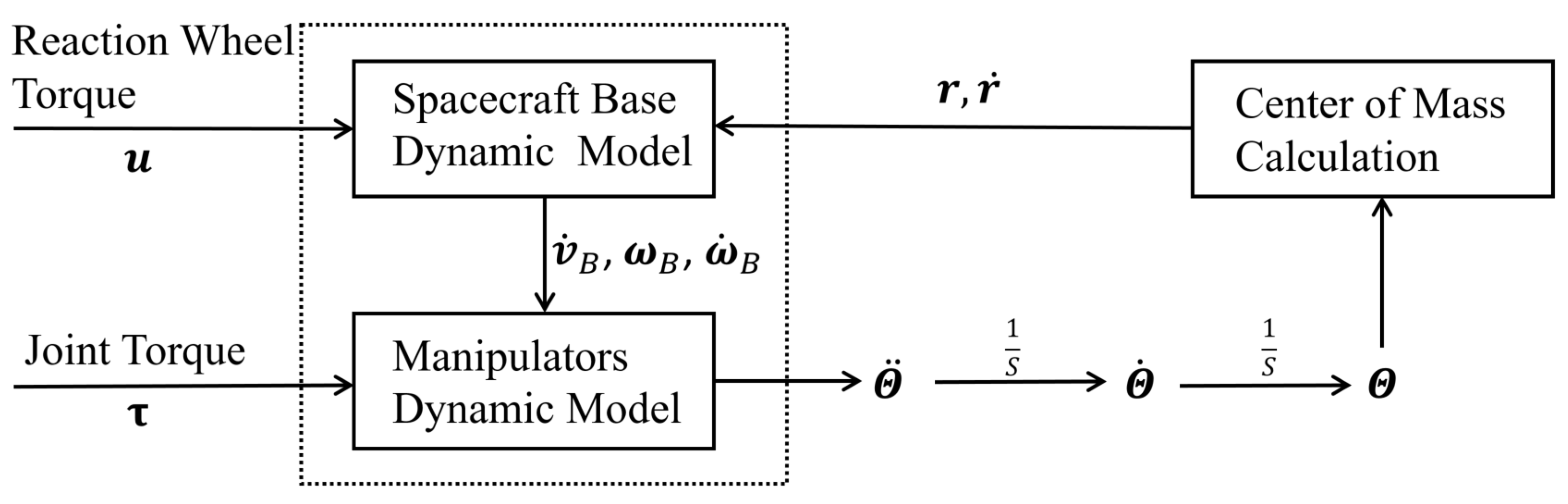
2. Modeling of Mini Space Robotic System

2.1. Problem Description

Similar to papers [20,34,35], the dynamic model of the mini space robot can be regarded as a number of different chain components connected to the satellite body. In this paper all components were considered as rigid bodies. A schematic diagram of the kinetic model is shown in Figure 1.

2.2. Kinematics and Dynamics

The dynamic model of the mini space robot is divided into two parts: a spacecraft base and n manipulators connected to the base.

2.2.1. Calculation of System’s Centroid Position

The VM method establishes a connection between the center of mass of the system and the satellite base using a virtual manipulator. The virtual manipulator is characterized by its kinematic properties rather than its dynamic properties. By determining the positions of each rigid body component of the mini space robot, the position of the system’s centroid is also determined. The position of the centroid can be mathematically expressed using Equation (1):
r 0 = i = 1 n [ m i ( i = 0 n 1 P i + P C i ) ] + m 0 P C 0 / i = 0 n m i
In Equation (1), P i denotes the vector representing the position of the i-th component body coordinate pointing to the (i+1)-th component. P C i represents the coordinates of the center of mass in the body coordinate system of the i-th component. By using this formulation, the total inertia of the system can be expressed as shown in Equation (2):
I C M = i = 0 n [ c I i + m i ( r i r i T E r i T r i ) ]
In Equation (2), c I i represents the inertia tensor of the centroid position in the body coordinate system of each component.

2.2.2. Kinematics of Spacecraft Base

Euler angles are commonly used to express the attitude of a rigid body [26]. In this paper, the specific sequence of rotations Z ( α ) Y ( β ) X ( γ ) is employed, where the attitude is described by the Euler angles Φ = [ α , β , γ ] T . The relationship between the time derivative of the Euler angles Φ and the angular velocity ω is given by:
ω = 0 s i n α c o s α c o s β 0 c o s α s i n α c o s β 1 0 s i n β α ˙ β ˙ γ ˙ = N ϕ Φ ˙
However, the singularity of Euler angles causes the rotational speed Φ ˙ to be unrepresented by ω , because N ϕ is irreversible when c o s α is equal to zero. To avoid singularity problems, quaternions are usually used to express the attitude of a rigid body [36], which can be expressed as Equation (4):
Q = q 0 q 1 q 2 q 3 T = q 0 q T T = c o s ψ 2 s i n ψ 2 e T T
In Equation (4), e represents the unit rotation axis, and ψ represents the rotation angle along e . The equation satisfies the condition q 0 2 + q T q = 1 . It is important to note that any rigid body attitude can be represented by both Q and Q . However, when π < ψ π (in radians) and q 0 > 0 are satisfied, the expressed attitude is unique. The time derivative of Q can be expressed as shown in Equation (5):
q 0 ˙ q ˙ = 1 2 q T q 0 E n + q × ω
where E n represents an identity matrix of size n × n , and q × is defined as:
q × = 0 q 3 q 2 q 3 0 q 1 q 2 q 1 0
ω can also be represented by Q as shown in Equation (6):
ω = 2 q 0 2 E 3 q 0 q × + q q T q 0 q ˙
Then, a 3 × 3 attitude matrix denoted as B i R can be used to represent the conversion between the coordinates of the inertial system and the base coordinate system. The linear velocity of the spacecraft base, deviating from the center of mass of the inertial system, can be expressed as shown in Equation (7):
B v B = r ˙ 0

2.2.3. Manipulator Chain Dynamics

By applying the kinematics of the spacecraft base, the dynamics of each manipulator can be modeled using the Newton–Euler method [13,18,24,37,38,39,40]. The angular and linear velocities of the ( i + 1 ) -th manipulator can be expressed in terms of the i-th manipulator, as shown in Equations (8) and (9):
i + 1 ω i + 1 = i i + 1 R i ω i + θ ˙ i + 1 i + 1 Z ^ i + 1
i + 1 v i + 1 = i i + 1 R i v i + i ω i × i P i + 1
where the superscript i denotes that the vector is represented in the i-th coordinate, i Z ^ i represents the unit vector of the rotation direction of the i-th axis, and i i + 1 R represents the rotation matrix from the ( i + 1 ) -th coordinate system to the i-th coordinate system. In Equation (9), i P i + 1 represents the position vector of the origin of the ( i + 1 ) -th coordinate system in the i-th coordinate system. The equations can also be expressed as follows:
v e ω e = J b v 0 ω 0 + J m Θ
where J b and J m are Jacobian matrices that map the velocities of the base and manipulator, respectively, to those of the end effector. They are defined as follows:
J b = E ( P e P 0 ) × O E R 6 × 6
J m = Z ^ 1 × ( P e P 1 ) Z ^ n × ( P e P n ) Z ^ 1 Z ^ n R 6 × n
The angular and linear acceleration of each component can be obtained according to Equations (8) and (9)
i + 1 ω ˙ i + 1 = i i + 1 R i ω ˙ i + i i + 1 R i ω i × θ ˙ i + 1 i + 1 Z ^ i + 1 + θ ¨ i + 1 i + 1 Z ^ i + 1
i + 1 v ˙ i + 1 = i i + 1 R i ( ω ˙ i × i P i + 1 + i ω i × i ω i × i P i + 1 + i v ˙ i )
Similarly, the linear acceleration at the center of mass of each component can be expressed as Equation (15)
i + 1 v ˙ C i + 1 = i + 1 ω ˙ i + 1 × i + 1 P C i + 1 + i + 1 ω i + 1 × i + 1 ω i + 1 × i + 1 P C i + 1 + i + 1 v ˙ i + 1
Finally, the total external force and torque on the i-th component can be expressed according to Newton’s equation and Euler’s equation:
i + 1 F i + 1 = m i + 1 i + 1 v ˙ C i + 1
i + 1 N i + 1 = C i + 1 I i + 1 i + 1 ω ˙ i + 1 + i + 1 ω i + 1 × C i + 1 I i + 1 i + 1 ω i + 1
where m i and C i I i represent the mass and the inertia matrix at the center of mass of the i-th connecting rod in its own coordinate system. i F i and i N i represent the resultant force and moment of the i-th component, respectively. Finally, the force relationship between adjacent components can be expressed as:
i f i = i + 1 i R i + 1 f i + 1 + i F i
i n i = i N i + i + 1 i R i + 1 n i + 1 + i P C i × i F i + i P i + 1 × i + 1 i R i + 1 f i + 1
where i f i and i n i represent the force and moment exerted by connecting rod i 1 on connecting rod i. The torque τ i at each joint can be expressed as Equation (20):
τ i = i n i T i Z ^ i
The conservation equations for the linear and angular momentum of the system can be written as follows:
P = m 0 v 0 + i = 1 n m i r ˙ i = P 0
L = C M I 0 C M ω 0 + r 0 × m 0 r ˙ 0 + i = 1 n C M I i C M ω i + r i × m i r ˙ i = L 0
where the linear and angular momenta are represented by P and L , respectively, with initial values P 0 and L 0 . The terms C M I i and C M ω i represent the inertial tensor and angular velocity of the i-th component in the inertial system. To summarize, the dynamic equation of the space robot can be expressed in the following state-space form (disregarding gravity effects):
τ = M Θ Θ ¨ + B Θ Θ ˙ Θ ˙ + C Θ Θ ˙ 2
where M Θ , B Θ , and C Θ are all complex functions about joint space Θ . Among them, M Θ R n × n is the mass matrix of manipulators, B Θ R n × n ( n 1 ) 2 is the Coriolis coefficient matrix, and C Θ R n × n is the centrifugal force’s coefficient matrix. In addition, Θ ˙ Θ ˙ and Θ ˙ 2 can be expressed by Equations (24) and (25):
Θ ˙ Θ ˙ = θ ˙ 1 θ ˙ 2 θ ˙ 1 θ ˙ 3 θ ˙ n 1 θ ˙ n T
Θ ˙ 2 = θ ˙ 1 2 θ ˙ 2 2 θ ˙ n 2 T
The dynamic equation of the mini space robot can be expressed using an alternative formulation, as shown in Equation (26):
M b M b m M m b M m Θ ¨ b Θ ¨ m + C b C b m C m b C m Θ ˙ b Θ ˙ m = B b 0 0 B m τ b τ m
Here, M b is the matrix corresponding to the overall spacecraft–manipulator system at a system configuration Θ . M m is the generalized mass matrix corresponding to the manipulator, and M b m = M m b T is the matrix representing the coupled inertia between the base and the manipulator.
If
τ = B Θ Θ ˙ Θ ˙ + C Θ Θ ˙ 2 ,
then there is
Θ ¨ = M 1 Θ τ τ
Thus, the forward dynamic system of the mini space robot is obtained. The dynamic simulation model of the mini space robot is illustrated in Figure 2.

3. Design of Parameter Adaptive Controller

In this section, the adaptive controller is designed based on the dynamics of the mini space robot. The reference model in the controller is assumed to be the same as the real physical model but the specific mass characteristic parameters cannot be determined. In order to enable the controller to update the dynamic parameters online, the linear separation of the parameters of the dynamic model is necessary.

3.1. Adaptive Controller Design

If the dynamic parameters are accurately known, the linearized equation represented by Y ( Θ , Θ ˙ , Θ ¨ ) π = u can be used to replace the inverse dynamics of the space robot, which facilitates the design of the controller. The feasibility of its inertial parameter separation is demonstrated in Appendix A. On the other hand, the linear separation expression is also convenient for a computer to iterate and update the parameters. Therefore, the nonlinear equation of motion can be expressed in a linear separation form with a suitable set of constant dynamic parameters such as Equation (29):
M Θ Θ ¨ + D Θ Θ ˙ = Y ( Θ , Θ ˙ , Θ ¨ ) π = u
where
D Θ Θ ˙ = B Θ Θ ˙ Θ ˙ + C Θ Θ ˙ 2
Assuming that the computational model and the kinetic model are consistent, the control law can be considered:
u = M Θ Θ ¨ r + D Θ Θ ˙ r + K D σ
where K D is a positive definite matrix; then, choose
Θ ˙ r = Θ ˙ d + Λ Θ ˜ Θ ¨ r = Θ ¨ d + Λ Θ ˜ ˙
where Λ is a positive definite matrix, and Θ ˙ d and Θ ¨ d represent the desired angular velocity and angular acceleration generated by the target trajectory. Θ ˙ r represents an intermediate reference variable generated by tracking the target angular velocity and angular acceleration, and the value of that variable is based on both the expected velocity and the position tracking error, and the representation of Θ ¨ r is the same. Equation (32) expresses the nonlinear compensation and coupling terms as functions of the desired velocity and acceleration, modified by the current state of the space robot. If
σ = Θ ˙ r Θ ˙ = Θ ˜ ˙ + Λ Θ ˜ ,
then substitute Equations (31) into (29) to obtain:
M Θ σ ¨ + D Θ σ ˙ + K D σ = 0
The Lyapunov function can be written as:
V ( σ , Θ ˜ ) = 1 2 σ T M Θ σ + 1 2 Θ ˜ T W Θ ˜ > 0 σ , Θ ˜ 0
where W R n × n is a symmetric positive definite matrix. The time derivative of V along the trajectory of Equation (34) is:
V ˙ = σ T M Θ σ ˙ + 1 2 σ T M ˙ Θ σ + Θ ˜ T W Θ ˜ ˙ = σ T K D σ + Θ ˜ T W Θ ˜ ˙
If W = 2 Λ K D is chosen, then:
V ˙ = Θ ˜ ˙ T K D Θ ˜ ˙ Θ ˜ T Λ K D Θ ˜
The formula is 0 if and only if Θ ˜ = 0 and Θ ˜ ˙ = 0 , thus indicating that the time derivative is negative definite. It can be seen that the origin of the state space Θ ˜ T σ T T is globally asymptotically stable, so the control law can be adaptively established according to the parameter vector π . The control law expressed by Equation (31) can be expressed as:
u = M ^ Θ Θ ¨ r + D ^ Θ Θ ˙ r + K D σ = Y ( Θ , Θ ˙ r , Θ ¨ r ) π ^ + K D σ
where π ^ represents the available estimate of the inertial parameter, and the corresponding M ^ and D ^ represent the estimated terms in the dynamic model.

3.2. Correction and Update of Inertial Parameters

The available inertial parameter vector π ^ cannot always accurately describe the mass characteristics of the system, and it is necessary to correct the parameters after obtaining the on-orbit control feedback information to improve the accuracy of the controller.

3.2.1. Recursive Least-Squares Method

On the premise that the state of the space robot system can be accurately feedback, the recursive least-squares method can identify the system parameters conveniently. After obtaining the torque and system state variables of each joint, the available inertial parameter vector π ^ of the k-th control cycle can be calculated according to the iterative least-squares method, as shown in Equation (39), which can be derived by the basic least-squares method:
π ^ k = π ^ k 1 + K k [ τ k Y k ( Θ k , Θ ˙ k , Θ ¨ k ) π ^ k 1 ]
where the gain matrix K k is shown in Equation (40):
K k = G k 1 Y k T [ Y k G k 1 Y k T + E ] 1
and the G k is the intermediate variable matrix:
G k = [ E K k Y k ] G k 1
Equation (39) shows that the parameter estimate π ^ at time k is equal to the parameter estimate pi at time k 1 plus a correction term, which is proportional to the difference between the torque vector measured at time k and Y k ( Θ k , Θ ˙ k , Θ ¨ k ) π ^ k 1 . The schematic diagram of the control loop based on the recursive least-squares parameter-adaptive controller is shown in Figure 3:

3.2.2. Parameter Update Based on Lyapunov’s Method

The key for the controller to identify inertial parameters is to provide an accurate parameter adaptation law, for which the Lyapunov method can provide an effective calculation method. According to Equation (38), the matrix Y does not depend on the actual value of the joint acceleration but on the expected value of the joint acceleration, so the problem of directly measuring the acceleration is avoided. Therefore, the Lyapunov function expressed by Equation (35) can be expressed as:
V ( σ , Θ ˜ , π ˜ ) = 1 2 σ T M Θ σ + 1 2 Θ ˜ T Λ K D Θ ˜ + 1 2 π ˜ T K π π ˜ > 0 σ , Θ ˜ , π ˜ 0
In Equation (42), the inertial parameter’s error vector term of the space robot is added to the Lyapunov function and K π is a symmetric positive definite matrix. The time derivative of V along the trajectory of the system is:
V ˙ = Θ ˜ ˙ T K D Θ ˜ ˙ Θ ˜ T Λ K D Θ ˜ + π ˜ T [ K π π ˜ ˙ Y k T ( Θ k , Θ ˙ k , Θ ¨ k ) σ ]
To make the last term of Equation (43) zero, we can make:
π ^ ˙ = K π 1 Y k T ( Θ k , Θ ˙ k , Θ ¨ k ) σ
Finally, the parameter adaptation law with Equation (38) as the control law in the mini space robot model represented by Equation (26) is obtained as:
π ^ ˙ = K π 1 Y k T ( Θ k , Θ ˙ k , Θ ¨ k ) ( Θ ˜ ˙ + Λ Θ ˜ )
The schematic diagram of the control loop of the parameter-adaptive controller based on the Lyapunov method is shown in Figure 4.

4. Numerical Simulation

In this section, an existing mini space robot with a four-DOF manipulator was modeled, as depicted in Figure 5. The satellite base and the antenna served as the primary objects of interest in the simulation presented in this paper. The satellite base requires precise positioning in a specific attitude, while the antenna’s center needs to be accurately oriented in a specified direction to fulfill mission-specific requirements.
Disregarding component interference, joints θ 1 , θ 3 , and θ 4 had a rotational range from −180° to 180° within their respective motion spaces, while joint 2 had a range from 0° to 180°. The installation positions and rotation ranges of the joints are illustrated in Figure 6. Table 1 presents the mass properties, centroid positions i P C i , and Denavit–Hartenberg parameters of the bodies. Furthermore, for the sake of convenience, a simplified model and component labeling were utilized. The spacecraft base was denoted as B 0 , while the accessory parts were labeled as B i (with subscripts). The coordinate positions of the mini space robot are depicted in Figure 7.

4.1. Influence of Prior Inertia Parameters on Controller Performance

The general orientation control task of a space robot is to perform attitude control while the manipulators are moving. In the first simulation, the mini space robot concurrently performed satellite attitude adjustment and end-effector antenna pointing tasks. This task exhibited generality in the on-orbit orientation of mini space robots, where other satellite-manipulator on-orbit maneuver modes can be regarded as submodes of this task. During this process, the controller utilized both the real inertial parameters and the prior inertial parameters with a certain level of error to control the same process. However, the controller did not update the parameters during the control process. Suppose the initial attitude of the mini space robot is Θ 0 = 0 0 0 90 45 45 0 and the target attitude is Θ f = 10 0 0 90 55 55 10 . Assume a certain ratio error exists between the prior inertial parameters and the actual parameters, following a normal distribution. In this paper, a three-time standard deviation was chosen as the error range, as shown below:
π p r i o r i N ( π r e a l , 1 3 η π r e a l )
where π p r i o r i and π r e a l represent the prior inertial parameters and real inertial parameters, respectively, and η represents the ratio of error in the prior inertial parameters. Initially, the controller carried out the orientation task using the real inertial parameters. The time-varying curves of the spacecraft base’s attitude and the angles of each joint are depicted in Figure 8.
The stability of the system under the control of the controller with real inertial parameters is demonstrated in Figure 8. Next, by setting η to 20 % , four different sets of a priori inertial parameters were randomly generated. Using the satellite’s attitude error as an example, Figure 9 illustrates the performance of the controller under these different sets of inertial parameters.
The red curve in Figure 9 represents the attitude error of the controller under the real inertial parameters, and the i π p r i o r i ’s, respectively, represent the corresponding control curves under the i-th group of prior inertia parameters. It can be seen from Figure 9 that without updating the prior parameters, inaccurate parameters lead to unstable control results. In addition, the inaccurate inertial parameters cause the controller to produce different degrees of overshoot, oscillation, slow convergence, and even divergence. It can be proved that the controller depends on the accuracy of the inertial parameters, and it is particularly important to obtain accurate inertial parameters or parameters that can be accurately equivalent to the system.

4.2. Influence of Weight Coefficient Λ on Controller Performance

The presence of Λ in Equation (32) allows the nonlinear compensation and coupling terms to be expressed as functions of desired velocity and acceleration, corrected by the current state of the spacecraft ( Θ ˙ and Θ ). Λ represents a velocity-dependent weight based on the desired velocity and position tracking error. Therefore, the value of Λ has a significant influence on the controller performance. In the second simulation, the real inertial parameters were also used as the preset parameters of the controller to carry out the same orientation process as the first simulation. Then, taking the satellite’s attitude error as an example, the control effect caused by different Λ ’s is studied in Figure 10.
This paper examined the convergence curve of the system when Λ varied from 0.4 to 2.0. Figure 10 shows that the influence of parameter Λ on the control effect is mainly manifested in two aspects: overshoot and convergence speed. Within a certain range, the smaller the value of Λ , the lower the dependence on the tracking error. At that time, the system has a faster response speed and greater overshoot.

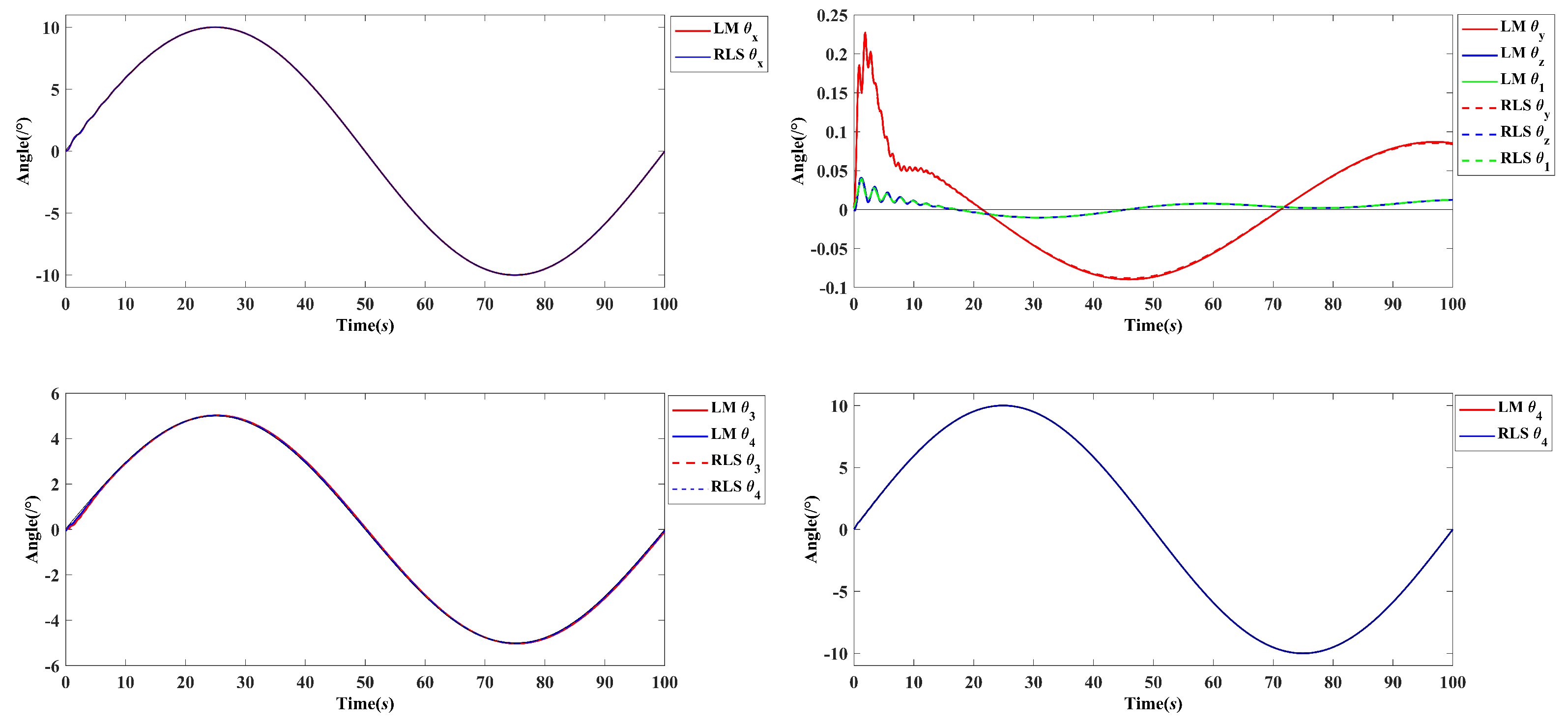
4.3. Inertial Parameter Update Using Recursive Least Square Method and Lyapunov Methods

Without loss of generality, the harmonic trajectories were tracked for each joint of the spacecraft in this part. The controller used recursive least-squares (RLS) and Lyapunov methods (LM) to adapt the inertial parameters during trajectory tracking, respectively. In addition, the stability of the two parameter adaptive methods was investigated by using the prior inertial parameters with different prior errors. Similar to the first part, we kept the y-axis and z-axis attitudes of the spacecraft base, and joint θ 1 was unchanged. At the same time, the attitude of the x-axis of the spacecraft base and the angles of θ 2 , θ 3 , and θ 4 tracked the sine-wave motion trajectory. The tracking process of both different parameter update methods is shown in Figure 11.
Figure 11 shows the tracking curves of the two methods when the error of the prior inertial parameter vector is 20 % . The black solid line in the figure represents the given tracking trajectory and the traces of the RLS and LM methods are distinguished using red and blue or solid and dashed lines, respectively. Both parameter update methods can track the given trajectory accurately, and the curves of the two methods have a high degree of coincidence. Since the most important difference between the RLS and the Lyapunov methods for updating parameters is whether there is torque feedback information, it was necessary to further investigate the influence of the accuracy of the prior parameters on the control results of the two different parameter updating methods. In this process, the change curves of the inertial parameters of the satellite base in the two control algorithms are shown in Figure 12. It can be seen from Figure 12 that the estimation accuracy of the inertial parameters of the LM method was worse than that of the RLS method because there was no torque feedback information. Of course, the rotation of the y-axis and z-axis of the satellite base was not involved in that process (only the attitude of the y-axis and z-axis was kept stable), so the correction of I y y and I z z by both methods was inaccurate. It can be further shown that that approximation can only correct the reference dynamic model in the direction of motion.
Hence, building upon the first part, the error in the prior inertial parameters was incrementally increased, and the performance of both parameter update methods in tracking a harmonic trajectory was compared once again. Six sets of different a priori inertial parameters were randomly generated within the range of η from 10 % to 40 % . The recursive least-squares (RLS) and Levenberg–Marquardt (LM) algorithms were employed to simulate the harmonic trajectory tracking for each parameter group. Subsequently, the tracking errors are presented in Figure 13 for comparison.
In Figure 13, the solid and dashed lines represent the tracking error curves of the recursive least-squares (RLS) and Levenberg–Marquardt (LM) methods, respectively. The results in Figure 13 demonstrate that when the error in the prior inertial parameters is small, the two parameter update methods exhibit similar control outcomes. However, as η gradually increases, the Lyapunov parameter update method introduces fluctuations, and the tracking error gradually increases during the convergence process. Conversely, the RLS method is less affected by the error in the prior parameters and only exhibits slight oscillations when η approaches 30 % .
Equations (39) and (44) show that neither the RLS nor the Lyapunov method can obtain the most accurate system inertial parameter vector in principle, which is different from the on-orbit inertial parameter identification. These methods only update the parameters to approximate the system dynamics captured by the Y ( Θ , Θ ˙ , Θ ¨ ) π term. From the simulation results, both the recursive least squares method and the Lyapunov method effectively adapted the inertial parameters, enabling the system to stably track the desired trajectory. The RLS-based parameter-adaptive controller maintained stable control performance even when the prior inertial parameters were highly inaccurate ( η = 40 % ), but this relied on accurate torque feedback for each joint. Additionally, in terms of computational resources, the Lyapunov method did not require matrix inversion operations during parameter updates. In practical applications, engineers typically strive to maintain the measurement error of inertial parameters for each component within the range of 5 % to 10 % . Within this range, controllers based on Lyapunov methods may offer certain advantages.
In addition, 10,000 repeated experiments were performed in Matlab to evaluate the computation time spent by the two algorithms in each control cycle, which is shown in Table 2. It can be seen that the average calculation time of the two algorithms was on the order of 10 4 s, which is far less than the control calculation period of the satellite on-orbit operation (the calculation period of the satellite on-orbit control algorithm is usually 0.25–1 s).

5. Conclusions

In this paper, a dynamic-approximation-based inertial-parameter-adaptive controller was studied for mini space robots. The dynamic model established by the combination of the VM method and Newton–Euler equations was proved to be able to play an important role in the numerical simulation and dynamics-based controller design. Two methods based on recursive least squares and Lyapunov were designed for updating the parameters of the adaptive controllers. It was verified by simulation that the accuracy of the inertial parameters had a significant impact on the performance of the controller. Moreover, the parameter Λ in the controller that expresses the degree of dependence on the current state of the system also had an important influence on the convergence characteristics of the system. Finally, the parameter update methods based on iterative least-squares and Lyapunov methods both showed a strong tracking ability in harmonic-tracking simulations. The difference was that the Lyapunov method had a poor adaptive ability to inaccurate prior inertial parameters, while the recursive least-squares method required more hardware resources such as accurate joint torque feedback and more computing power. The inertial-parameter-adaptive controller proposed in this paper can accurately approximate the dynamics of mini space robots and has certain application prospects in this field.

Author Contributions

Conceptualization, Y.L. and L.T.; methodology, Y.L. and L.T.; software, Y.L. and L.T.; validation, Y.L. formal analysis, Y.L. and Z.J.; investigation, Y.L. and Z.J.; resources, Y.L.; data curation, Y.L. and L.T.; writing—original draft preparation, Y.L. and L.T.; writing—review and editing, Y.L. and Z.J.; visualization, Y.L.; supervision, L.T.; project administration, Z.J.; funding acquisition, Z.J. All authors have read and agreed to the published version of the manuscript.

Funding

This research was funded by Key Laboratory of Micro-Nano Satellite Research Zhejiang Province and Huanjiang Laboratory.

Acknowledgments

This research was supported by “Zhejiang Provincial Key Laboratory of Micro-nano Satellite Research”.

Conflicts of Interest

There is no conflict of interest.

Appendix A

The dynamic equations derived by the Newton–Euler method are not linear equations with respect to the inertial parameters. The existence of the m i i P C i 2 term in Equation (19) makes the inertial parameters and dynamics nonlinear, so in order to eliminate this term, Equation (19) can be transformed:
i N i + i P C i × i F i = C i I i i ω ˙ i + i ω i × ( C i I i i ω i ) + i P C i × ( m i i v ˙ C i ) = C i I i i ω ˙ i + i ω i × ( C i I i i ω i ) + m i i P C i × [ i v ˙ i + i ω ˙ i × i P C i + i ω i × ( i ω i × i P C i ) ]
The third term in Equation (A1) can be expanded to obtain:
m i i P C i × [ i v ˙ i + i ω ˙ i × i P C i + i ω i × ( i ω i × i P C i ) ] = m i i P C i × i v ˙ i + m i i P C i × ( i ω ˙ i × i P C i ) + m i i P C i × [ i ω i × ( i ω i × i P C i ) ]
The terms m i i P C i × ( i ω ˙ i × i P C i ) and m i i P C i × [ i ω i × ( i ω i × i P C i ) ] in Equation (A2) can be written as:
m i i P C i × ( i ω ˙ i × i P C i ) = i P C i × ( i ω ˙ i × m i i P C i ) = m i ( i P C i T i P C i E i P C i i P C i T ) i ω ˙ i
and:
m i i P C i × [ i ω i × ( i ω i × i P C i ) ] = i ω i × [ i P C i × ( i ω i × m i i P C i ) ] + ( i ω i × m i i P C i ) × ( i ω i i P C i ) = i ω i × [ m i ( i P C i T i P C i E i P C i i P C i T ) i ω ˙ i ]
Applying the parallel axis theorem, Equation (29) can be expressed as:
i N i + i P C i × i F i = C i I i i ω ˙ i + i ω i × ( C i I i i ω i ) + m i i P C i × i v ˙ i + m i ( i P C i T i P C i E i P C i i P C i T ) i ω ˙ i + i ω i × [ m i ( i P C i T i P C i E i P C i i P C i T ) i ω ˙ i ] = O i I i i ω ˙ i + i ω i × ( O i I i i ω i ) + m i i P C i × i v ˙ i
Thus, Equation (19) can be expressed in the form of Equation (A6):
i n i = O i I i i ω ˙ i + i ω i × ( O i I i i ω i ) + m i i P C i × i v ˙ i + i + 1 i R i + 1 n i + 1 + i P i + 1 × i + 1 i R i + 1 f i + 1
Then, the inertia parameter of the i-th component can be represented by a vector:
π i = O i I x x O i I x y O i I x z O i I y y O i I y z O i I z z m i i P C i x m i i P C i y m i i P C i z m i T
Now, the equation does not contain the m i i P C i 2 term. The dynamic equation of the end part can be linearly separated as:
n n n = K ( n ω ˙ n ) + S ( n ω n ) K ( n ω n ) S ( n v ˙ n ) 0 π n
where the functions K ( a ) and S ( a ) are expressed as:
K ( a ) = a x a y a z 0 0 0 0 a x 0 a y a z 0 0 0 a x 0 a y a z S ( a ) = 0 a z a y a z 0 a x a y a x 0
The torque of each joint of the space robot can be expressed as Equation (A9), and Y i j in the coefficient matrix is summarized as Equation (A10):
b n b 1 n 1 2 n 2 n n n = Y b b Y b 1 Y b 2 Y b n 0 Y 11 Y 12 Y 1 n 0 0 Y 22 Y 2 n 0 0 0 Y n n π b π 1 π 2 π n
Y i j = K ( i ω ˙ i ) + S ( i ω i ) K ( i ω i ) S ( i v ˙ i ) 0 i = j K ( i ω ˙ j ) + S ( i ω j ) K ( i ω j ) S ( i ω ˙ j ) + S ( i ω j ) S ( i ω j ) S ( i v ˙ j ) i v ˙ j i j
Equation (A9) is abbreviated as:
τ = Y ( Θ , Θ ˙ , Θ ¨ ) π
where Y is a function of the mini space robots Θ , Θ ˙ , and Θ ¨ , and only the kinetic parameters are included in π .

References

  1. Nakasuka, S.; Miyata, K.; Tsuruda, Y.; Aoyanagi, Y.; Matsumoto, T. Discussions on attitude determination and control system for micro/nano/pico-satellites considering survivability based on Hodoyoshi-3 and 4 experiences. Acta Astronaut. 2018, 145, 75–174. [Google Scholar] [CrossRef]
  2. Zhang, X.; Liu, J.; Tong, Y.; Liu, Y.; Ju, Z. Attitude Decoupling Control of Semifloating Space Robots Using Time-Delay Estimation and Supertwisting Control. IEEE Trans. Aerosp. Electron. Syst. 2021, 57, 4280–4295. [Google Scholar] [CrossRef]
  3. Jin, R.; Rocco, P.; Chen, X.; Geng, Y. LPV-Based Offline Model Predictive Control for Free-Floating Space Robots. IEEE Trans. Aerosp. Electron. Syst. 2021, 57, 3896–3904. [Google Scholar] [CrossRef]
  4. Chu, X.; Hu, Q.; Zhang, J. Path Planning and Collision Avoidance for a Multi-Arm Space Maneuverable Robot. IEEE Trans. Aerosp. Electron. Syst. 2021, 54, 217–232. [Google Scholar] [CrossRef]
  5. Virgili-Llop, J.; Drew, J.V.; Zappulla, I.R.; Romano, M. Laboratory experiments of resident space object capture by a spacecraft–manipulator system-ScienceDirect. Aerosp. Sci. Technol. 2017, 71, 530–545. [Google Scholar] [CrossRef]
  6. Jorgensen, G.; Bains, E. SRMS History, Evolution and Lessons Learned. In Proceedings of the AIAA SPACE 2011 Conference & Exposition, Long Beach, CA, USA, 27–29 September 2011. [Google Scholar]
  7. Landzettel, K. MSS Ground Control Demo with MARCO. In Proceedings of the 6th International Symposium on Artificial Intelligence, Robotics and Automation in Space: iSAIRAS 2001, Montreal, QC, Canada, 18–21 June 2001. [Google Scholar]
  8. Stieber, E.M.; Hunter, G.D.; Abramovici, A. Overview of the Mobile Servicing System for the International Space Station. Artif. Intell. Robot. Autom. Space 1999, 440, 37–42. [Google Scholar]
  9. Stieber, M.F.; Trudel, C.P.; Hunter, D.G. Robotic systems for the International Space Station. In Proceedings of the International Conference on Robotics and Automation, Albuquerque, NM, USA, 25 April 1997; pp. 3068–3073. [Google Scholar]
  10. Sasiadek, J.Z. Space robotics and manipulators—The past and the future. Control Eng. Pract. 1994, 2, 491–497. [Google Scholar] [CrossRef]
  11. Piedboeuf, J.C.; Carufel, J.D.; Aghili, F.; Dupuis, E. Task verification facility for the Canadian special purpose dextrous manipulator. In Proceedings of the IEEE International Conference on Robotics and Automation, Detroit, MI, USA, 10–15 May 2002; pp. 1077–1083. [Google Scholar]
  12. Wanga, X.; Shi, L.; Katupitiya, J. Coordinated Control of a Dual-arm Space Robot to Approach and Synchronise with the Motion of a Spinning Target in 3D Space. Acta Astronaut. 2020, 176, 99–110. [Google Scholar] [CrossRef]
  13. Moghaddam, B.M.; Chhabra, R. On the guidance, navigation and control of in-orbit space robotic missions: A survey and prospective vision. Acta Astronaut. 2021, 184, 70–100. [Google Scholar] [CrossRef]
  14. Yoji, U.; Yoshida, K. Resolved motion rate control of space manipulators with generalized Jacobian matrix. IEEE Trans. Robot. Autom. 1989, 5, 303–314. [Google Scholar]
  15. Nenchev, D.; Umetani, Y.; Yoshida, K. Analysis of a Redundant Free-Flying Spacecraft/Manipulator System. IEEE Trans. Robot. Autom. 1992, 8, 1–6. [Google Scholar] [CrossRef]
  16. Dubowsky, S.; Papadopoulos, E. The kinematics, dynamics, and control of free-flying and free-floating space robotic systems. Robot. Autom. IEEE Trans. 1993, 9, 531–542. [Google Scholar] [CrossRef]
  17. Liang, B.; Xu, Y.; Bergerman, M. Mapping a space manipulator to a dynamically equivalent manipulator. J. Dyn. Syst. Meas. Control 1998, 120, 1–7. [Google Scholar] [CrossRef] [Green Version]
  18. Yoshida, K.; Kurazume, R.; Umetani, Y. Dual arm coordination in space free-flying robot. In Proceedings of the ICRA, Sacramento, CA, USA, 9–11 April 1991. [Google Scholar]
  19. Papadopoulos, E.; Moosavian, S. Dynamics and control of multi-arm space robots during chase and capture operations. In Proceedings of the IEEE/RSJ International Conference on Intelligent Robots and Systems, Munich, Germany, 12–16 September 1994. [Google Scholar]
  20. Yang, S.; Zhang, Y.; Chen, T.; Wen, H.; Jin, D. Assembly Strategy for Modular Components Using a Dual-Arm Space Robot with Flexible Appendages. Aerospace 2022, 9, 819. [Google Scholar] [CrossRef]
  21. Walker, M.W.; Wee, L.B. Adaptive control of space-based robot manipulators. Robot. Autom. IEEE Trans. 1991, 7, 828–835. [Google Scholar] [CrossRef]
  22. Wee, L.B.; Walker, M.W.; Mcclamroch, N.H. An articulated-body model for a free-flying robot and its use for adaptive motion control. Robot. Autom. IEEE Trans. 1997, 13, 264–277. [Google Scholar]
  23. Liu, D.; Chen, L. Space Robot On-Orbit Operation of Insertion and Extraction Impedance Control Based on Adaptive Neural Network. Aerospace 2023, 10, 466. [Google Scholar] [CrossRef]
  24. Wu, X.; Zhao, H.; Huang, B.; Li, J.; Liu, R. Minimum-learning-parameter-based anti-unwinding attitude tracking control for spacecraft with unknown inertia parameters. Acta Astronaut. 2021, 179, 498–508. [Google Scholar] [CrossRef]
  25. Ls, A.; He, Y.B.; Ms, C.; Qg, D.; Xin, J.A. Robust control of a space robot based on an optimized adaptive variable structure control method. Aerosp. Sci. Technol. 2022, 120, 107267. [Google Scholar]
  26. Xu, W.; Hu, Z.; Zhang, Y.; Liang, B. On-orbit identifying the inertia parameters of space robotic systems using simple equivalent dynamics. Acta Astronaut. 2017, 132, 131–142. [Google Scholar] [CrossRef]
  27. Nabavi-Chashmi, S.Y.; Malaek, M.B. On the identifiability of inertia parameters of planar Multi-Body Space Systems. Acta Astronaut. 2018, 145, 199–215. [Google Scholar] [CrossRef]
  28. Ma, O. On-Orbit Identification of Inertia Properties of Spacecraft Using Robotics Technology. 2006. Available online: https://www.researchgate.net/publication/235063328_On-Orbit_Identification_of_Inertia_Properties_of_Spacecraft_using_Robotics_Technology (accessed on 24 June 2023).
  29. Nainer, C.; Garnier, H.; Gilson, M.; Evain, H.; Pittet, C. Parameter estimation of a gyroless micro-satellite from telemetry data. Control Eng. Pract. 2022, 123, 105–134. [Google Scholar] [CrossRef]
  30. Nuthi, P.; Subbarao, K. Computational adaptive optimal control of spacecraft attitude dynamics with inertia matrix identification. In Proceedings of the American Control Conference, Boston, MA, USA, 6–8 July 2016. [Google Scholar]
  31. Chang, H.; Huang, P.; Lu, Z.; Zhang, Y.; Meng, Z.; Liu, Z. Inertia Parameters Identification for Cellular Space Robot through Interaction. Aerosp. Sci. Technol. 2017, 71, 464–474. [Google Scholar] [CrossRef]
  32. Yao, X.; Gang, T.; Ma, Y.; Qi, R. An adaptive actuator failure compensation scheme for spacecraft with unknown inertia parameters. In Proceedings of the Decision & Control, Maui, HI, USA, 10–13 December 2012. [Google Scholar]
  33. Lei, R.H.; Chen, L. Adaptive fault-tolerant control based on boundary estimation for space robot under joint actuator faults and uncertain parameters. Def. Technol. 2019, 5, 964–971. [Google Scholar] [CrossRef]
  34. Huang, P.; Wang, M.; Meng, Z.; Zhang, F.; Liu, Z. Attitude takeover control for post-capture of target spacecraft using space robot. Aerosp. Sci. Technol. 2016, 51, 171–180. [Google Scholar] [CrossRef]
  35. Palma, P.; Seweryn, K.; Rybus, T. Impedance Control Using Selected Compliant Prismatic Joint in a Free-Floating Space Manipulator. Aerospace 2022, 9, 406. [Google Scholar] [CrossRef]
  36. Ulrich, S.; Sasiadek, J.Z.; Barkana, I. Nonlinear adaptive output feedback control of flexible-joint space manipulators with joint stiffness uncertainties. J. Guid. Control Dyn. 2014, 37, 1961–1975. [Google Scholar] [CrossRef] [Green Version]
  37. Marchionne, C.; Sabatini, M.; Gasbarri, P. GNC architecture solutions for robust operations of a free-floating space manipulator via image based visual servoing. Acta Astronaut. 2021, 180, 218–231. [Google Scholar] [CrossRef]
  38. Liu, Y.; Jin, Z.; Teng, L. PSO-Based Time Optimal Rapid Orientation for Micronano Space Robot. IEEE Trans. Aerosp. Electron. Syst. 2023, 59, 1921–1934. [Google Scholar] [CrossRef]
  39. Zhang, X.; Ling, K.; Lu, Z.; Zhang, X.; Liao, W.; Lim, W. Piece-wise affine MPC-based attitude control for a CubeSat during orbital manoeuvres. Aerosp. Sci. Technol. 2021, 118, 106997. [Google Scholar] [CrossRef]
  40. Oestreich, C.E.; Linares, R.; Gondhalekar, R. Tube-Based Model Predictive Control with Uncertainty Identification for Autonomous Spacecraft Maneuvers. J. Guid. Control Dyn. 2023, 46, 6–20. [Google Scholar] [CrossRef]
Figure 1. General model of a mini space robot.
Aerospace 10 00679 g001
Figure 2. Schematic diagram of the dynamic model of the mini space robot.
Aerospace 10 00679 g002
Figure 3. Recursive least-squares parameter-adaptive controller.
Aerospace 10 00679 g003
Figure 4. Lyapunov method based parameter-adaptive controller.
Aerospace 10 00679 g004
Figure 5. Mini space robot model.
Aerospace 10 00679 g005
Figure 6. Schematic diagram of the joint’s installation position and rotation.
Aerospace 10 00679 g006
Figure 7. Simplified model of the space robot.
Aerospace 10 00679 g007
Figure 8. Orientation process under real inertial parameters.
Aerospace 10 00679 g008
Figure 9. Attitude control error under different inertial parameters.
Aerospace 10 00679 g009
Figure 10. Influence of weight coefficient Λ on controller performance.
Aerospace 10 00679 g010
Figure 11. Tracking curves of the two methods.
Aerospace 10 00679 g011
Figure 12. Inertia parameter’s change curve.
Aerospace 10 00679 g012
Figure 13. Comparison of the adaptability of the prior inertia parameters of the two methods to different initial errors.
Aerospace 10 00679 g013
Table 1. The mass properties of the space robotic system.
Parameters B 0 B 1 B 2 B 3 B 4
Mass (kg) 131.7342.08224.56925.280134.078
i P C i (m) i x −0.04500.4960.5000.149
i y 0.1010000
i z −0.0610.035000
i I i ( kg · m 2 ) I x x 7.6100.0030.0170.01736.254
I y y 11.7210.0031.9492.09018.637
I z z 11.4040.0021.9592.10118.637
I x y −1.7730000
I x z 1.7990000
I y z 0.6520000
Twist angle α i (rad) 00 π / 2 00
Length of links a i (m) 0.3200.0561.0001.0000
Offset of links links d i (m) 00000
Joint angle θ i (rad) [ α , β , γ ] T θ 1 ( t ) θ 2 ( t ) θ 3 ( t ) θ 4 ( t )
Table 2. Algorithm calculation time comparison.
Calculation MethodCalculation Time(s)
MeanVarMaxMin
RLS3.202 × 10 4 7.736 × 10 8 22.63 × 10 3 2.187 × 10 4
LM2.440 × 10 4 1.325 × 10 8 6.405 × 10 3 1.832 × 10 4
Disclaimer/Publisher’s Note: The statements, opinions and data contained in all publications are solely those of the individual author(s) and contributor(s) and not of MDPI and/or the editor(s). MDPI and/or the editor(s) disclaim responsibility for any injury to people or property resulting from any ideas, methods, instructions or products referred to in the content.

