A Rapid Surrogate Model for Estimating Aviation Noise Impact across Various Departure Profiles and Operating Conditions

Abstract

Aviation noise remains a key barrier to the sustainable growth of commercial aviation. The advent of emerging technologies, such as urban air mobility, and the renewed interest in commercial supersonic transport aircraft, has only further raised concerns over the resultant community noise exposure. The foundation of any noise mitigation effort is the ability to accurately model noise metrics over a wide range of scenarios. Aviation noise is influenced by a wide variety of factors, including aircraft type, payload weight, thrust settings, airport elevation, ambient weather, and flight trajectory. Traditional noise modeling paradigms rely on physics-based and empirical calculations, which are computationally expensive. Attempts at speeding up the computations with alternate models could deliver on speed or accuracy, but not both. Recent research has indicated that model order reduction techniques hold promise for transforming and greatly reducing the number of quantities that need to be modeled. Paired with surrogate modeling techniques, a rapid and accurate noise model can be generated. The research presented in this manuscript expands on the model order reduction method and develops a rapid noise surrogate model, which can account for the piloting actions, the ambient temperature, and airport elevation. The presented results indicate that the method works well with minimal error for most modeling scenarios. The results also outline avenues for improvement, such as using a different class of surrogate models or modeling additional training cases. The model developed in this research has numerous applications for multi-query applications, such as parametric trade-off analyses and optimization studies. With the inclusion of airport and aircraft parameters, the model enables the development of frameworks that optimize piloting actions for noise mitigation on the ground.

1. Introduction

According to the U.S. Federal Aviation Administration (FAA), commercial aviation has historically been tied to economic activity, and a return of passenger numbers to pre-pandemic operation levels will be expected towards the middle of the decade [1]. As aircraft operations are expected to recover and continue to grow, issues associated with commercial aviation are likewise expected to grow in scope. An increase in air traffic demand by an average of 4.0 percent annually is expected by various government and industry stakeholders [1,2,3]. As this trend continues, the severity of associated environmental impacts will also increase. One of these impacts is community exposure to aviation noise, which has posed a significant obstacle for the aviation industry. Noise is extremely difficult to model and mitigate due to the complexity of its behavior, in relation to both aircraft performance [4] and propagation through the atmosphere [5].

There are many concerns surrounding aviation noise impact, ranging from public annoyance to potential long-term health effects [6]. The mitigation of aviation noise is, therefore, desirable, due to the scale and significance of the problem [7]. For that reason, research into noise abatement and mitigation has seen significant investments from academia, manufacturers, and regulatory agencies. Much of the existing research is based on aircraft design, specifically focusing on new technologies built into new designs or mounted as retrofits to existing aircraft. Another key area of research involves improvements in operational efficiencies. Design methodologies and tools that can better model the noise output of an aircraft in a wide variety of scenarios are also topics of research in the field.

During aircraft operation, the intensity of noise emitted from an aircraft varies based on the aircraft’s takeoff and landing procedures [8]. In particular, the noise impact from a departure is characterized by high levels of engine usage whereas arrival noise is characterized by lower thrust levels, and a longer exposure duration. For departure operations, there is higher variability in the aircraft trajectory and performance characteristics compared to arrivals, where the final approach must be maintained at a $3^{\circ }$ glide slope. These additional degrees of freedom from the aircraft trajectory also add the potential for additional optimization constraints, such as fuel burn or minimization of emissions. A methodology that would improve the computational efficiency of existing processes of determining noise outputs based on aircraft operational parameters is highly desirable. A noise metric output could quickly be obtained with such a methodology, given a set of aircraft operational parameters. Thus, such a methodology would enable multi-query applications, such as parametric trade-off analyses and optimization studies. The potential use of such a methodology would be the development of optimal noise abatement profiles, given the constraints of operating conditions and aircraft capabilities.

The objective of the research presented in this manuscript is the development of a new aircraft noise model to help improve noise abatement research and operations at airports. This manuscript provides details about the development of such a model, how the model performs when compared to traditional noise models, and the errors associated with the model. This research also builds upon the relatively scarce available literature on the application of model order reduction techniques to the aviation noise quantification process.

2. Background and Literature Review

This section presents the necessary background and summarizes the available relevant literature pertinent to aviation noise estimation.

2.1. Aviation Noise—Influencing Factors

Aviation noise is influenced by a number of factors, which are categorized into two separate groups within the context of this research. The first group includes factors that can be controlled, to some extent, by the pilot or operator of an aircraft, which are hereby referred to as internal parameters for a departure operation.

The altitude of thrust cutback, for example, is one of these internal parameters, which significantly affects noise metrics [9]. Another internal parameter would be the altitude of acceleration initiation, i.e., the altitude at which the aircraft pitches over and starts accelerating, while maintaining a positive climb rate. In this state, the aircraft gains airspeed and retracts flaps based on its flap schedule. The reduction of takeoff and/or climb thrust is another pilot-controllable parameter with a major influence on aircraft trajectory and engine source noise. Thrust reduction is another controllable parameter that significantly affects departure performance and noise. Operators have the option to utilize reduced thrust during takeoff and climb to prolong engine life and reduce noise impact. The amount of thrust reduction also affects the climb performance and distance covered during the take-off ground roll. Combinations of different parameter values lead to different noise abatement departure procedure definitions [10,11].

The aircraft performance can be modeled by the sum of the aircraft’s potential and kinetic energy [12]. Parameters such as speed and climb rate can be condensed into their corresponding kinetic and potential energy representations. Since excess power is needed to either accelerate or climb, an accurate representation of a climbing aircraft’s performance can be quantified based on how much excess power is being dedicated for either purpose, called the energy share percentage. The relation between the energy share percent, acceleration, and climb is described in Equation (1), where G is the climb gradient, $G_m$ represents the maximum available acceleration as a fraction of the standard acceleration due to gravity, and $A_p$ is the energy share percent value.

$$G=G_m\left(1-\frac{A_p}{100}\right)$$

(1)

The other important parameters that need to be accounted for are external to the flight and cannot be controlled by the pilot. The takeoff gross weight of the aircraft is one of these external parameters. Weight has a significant effect on the thrust and lift characteristics of the aircraft, as more thrust is needed to maintain similar levels of performance with a heavier aircraft, which has cascading effects on noise metrics.

The takeoff gross weight is determined by three quantities: the operating empty weight, payload weight, and fuel weight. Although the operating empty weight is the only “fixed” quantity, there is typically no room for flexibility on fuel weight, which depends on the mission to be flown and reserve requirements. It is also uneconomical to reduce the payload of a commercial aircraft for a noise mitigation effect. Additionally, both aircraft performance [13] and the propagation of sound [14] through the atmosphere can be affected by factors such as ambient temperature, humidity, and air density. Most noise models account for these factors by defining the airport of operation through its elevation above mean sea level and a weather profile. Accounting for the weather and elevation is important in aviation noise modeling and optimization [15]. The ambient temperature, for example, is one of the most dominant factors when modeling aviation noise [16,17].

2.2. Current Noise Modeling Paradigms

Aviation noise modeling is typically done with the use of physics-based equations and semi-empirical models, often programmed into software packages. One such commonly used tool is the Aviation Environmental Design Tool (AEDT) developed by the FAA [18,19]. AEDT is a comprehensive tool used for environmental analysis, which includes an aircraft performance model and environmental models to compute noise, emissions, fuel consumption, and air quality metric results.

In order to model the environmental impacts, various trajectory and performance characteristics of the flight are required. If real-world data are available, each flight can be modeled uniquely with fixed-point profile definitions. Each fixed-point profile is a sequence of points specifying the aircraft’s ground track distance, altitude, speed, and thrust. Alternatively, a procedural profile definition, in conjunction with an aircraft performance model may be used. These profiles are defined as a series of steps that describes the state of the aircraft during a departure or arrival operation. For a departure operation, steps would include a take-off ground roll, followed by various constant speed or accelerated climbs. Parameters for such a procedural profile definition would include takeoff thrust levels, climb rates, target altitudes, target speeds, and energy share percentages.

Once a flight, or a set of flights, has been modeled, metrics such as fuel consumption, emissions, and noise can be computed from the resultant trajectories and performance. To compute aviation noise impacts, a user-defined receptor grid is created and geographically placed around the airport and the departure ground track. The selected noise metric is then computed at each point in the receptor grid. A sufficiently large number of points with adequate density is needed to perform noise contour analysis.

AEDT and other similarly structured noise tools can account for variations in the aircraft type, ground track, weather, airport elevation, and vertical profile. However, in order to be accurate over a wide variety of conditions, these tools have to rely on physics-based and semi-empirical models. The comprehensiveness of these tools also makes it difficult for fast and efficient computations of noise metrics. This issue of computational complexity has been a limitation with previous studies, where clustering of operations to reduce the amount of modeling effort [20] or the evaluation of a handful of alternatives as opposed to a true comprehensive optimization effort [15] have been observed.

2.3. Attempts at Rapid Noise Estimation

In order to create a rapid noise estimation model, a few different methods have been proposed, which are briefly described here.

Bernardo [21] proposed the creation of a pre-computed library consisting of aircraft-level SEL dB noise grids. These grids are then rotated and aligned with different runway configurations and superimposed to generate airport-level noise grid results. The core improvement came from the pre-computed library, which negated the need for evaluating the aircraft performance, noise–power–distance look-ups and interpolation, and noise propagation models. This method, called the airport noise grid interpolation method (ANGIM), was made feasible with several simplifying assumptions, i.e., straight tracks, sea-level airports, standard day weather, etc. However, these simplifying assumptions have also led to lower model accuracy conditions in conditions outside of the assumptions.

To improve the accuracy of this model, calibration models were proposed, which applied correction factors to the noise metrics predicted by the ANGIM method. Calibration models were proposed for averaged generic vehicle definitions [22], curved ground tracks [23], and atmospheric conditions [24]. These calibration models were based on regression models, such as response surface equations (RSEs), Kriging interpolation, and artificial neural networks. A common theme amongst these studies was the trade-off between the model’s accuracy and speed. For example, a second-order RSE proved to be fast but inaccurate, whereas higher-order RSEs would be accurate but too expensive to train and evaluate.

Therefore, although several attempts have been made in the literature to create rapid noise models, the ability to accurately and rapidly evaluate aviation noise metrics in a wide range of modeling scenarios has remained elusive.

2.4. Model Order Reduction Techniques

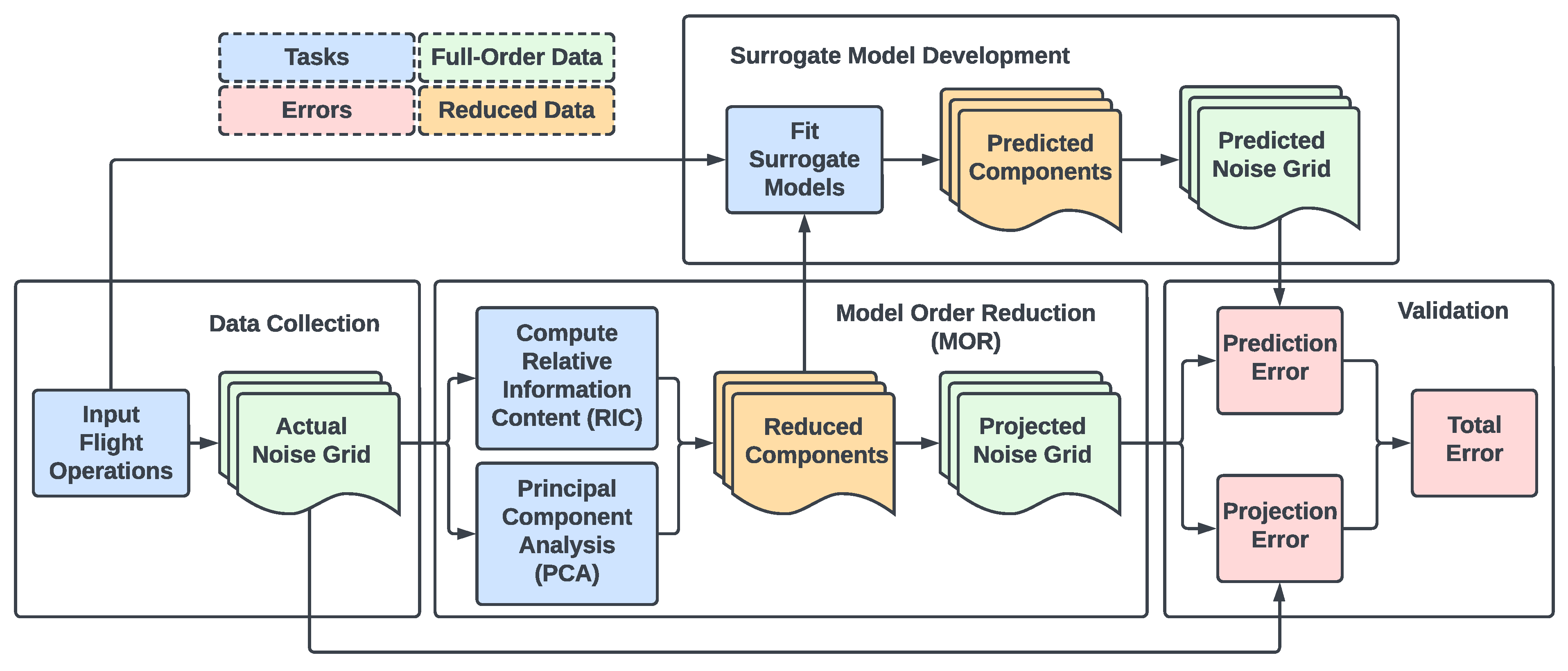
In order to speed up the aviation noise computation process, a transformation of the problem is needed. Fundamentally, a reduction in the complexity of the computation would make the process faster and more efficient. In the literature, the collection of methods used for this purpose is referred to as model order reduction (MOR) techniques. These techniques reduce the amount of data to be predicted by transforming the problem into a lower-dimensional representation. In doing so, the original data are approximated with some loss of information. Various MOR techniques vary in how they define and minimize the error associated with this transformation.

Although the concept of model order reduction is quite mature, its application to aviation noise modeling remains limited. In other aerospace disciplines, MOR has found use in design space exploration [25], design optimization [26], evaluation of aerodynamic loads [27], solid mechanics and structural assessment [28], and aeroelasticity [29].

In the context of aviation noise, the limited application of the principal component analysis (PCA) has shown significant promise. Previous studies have shown that the use of the PCA method on a large set of aviation noise grid results can successfully reduce the dimensionality of the problem and enable real-time aviation noise result computations [16,30,31]. These previous studies have mostly focused on creating models, which include the controllable parameters discussed in Section 2.1, while excluding uncontrollable factors such as ambient temperature conditions or airport elevation. As these uncontrollable factors play a significant role in the magnitude of noise metrics, a MOR-based methodology, which can include these factors, is desirable.

3. Methodology

This section outlines the steps of the developed methodology. A complete flowchart of the process is shown in Figure 1. The process can broadly be split into four parts. The first part involves the collection of data used to build the model, the second is the use of model order reduction to reduce model complexity, the third part is the creation of a surrogate model to perform rapid evaluations of the reduced model, and the fourth part is the validation of the methodology, with an analysis of the introduced errors.

3.1. Data Collection

The first step of the process is the collection of noise grid data obtained from any noise tool or noise measurements. Typically, a large number of solutions are required, and these solutions should correspond to cases with a good variety across the influencing parameters. A requirement of this step is that all solutions be computed on the same noise grid definition, i.e., the number of receptors in the grid, and their locations must stay the same across all modeling cases.

Once the noise grid results are obtained, they are represented as vectors, with each component of the vector representing a particular receptor within the grid. These vectors are hereby referred to as snapshots, represented by $w_i$, where $w$ is the vector representation of a noise grid and i is an index for the modeling case. A typical noise contour analysis requires grid definitions comprising tens or hundreds of thousands of receptors. The length of the corresponding snapshot representation is the same as the number of receptors in the grid definition.

The complete set of snapshots is assembled into a snapshot matrix $\mathit{W}$ whose columns are individual snapshots $w_i$ minus the mean snapshot $\overline{w}$. This subtraction of the mean snapshot is conducted to move the origin of the high-dimensional space to the mean snapshot and, thus, center the high-dimensional snapshot data.

3.2. Model Order Reduction

Principal component analysis (PCA) is utilized here for model order reduction (MOR) by selecting a subset of principal axes that serve as the bases for representing noise grid results. The high-dimensional noise grid data are then reoriented along these chosen principal axes. The principal axes ensure that much of the information encoded in the dataset is captured along a few axes, while a vast majority of axes can be dropped from consideration [32]. This results in a projection of the original high-dimensional vector snapshot to a vector with much fewer components.

Using singular value decomposition (SVD), the snapshot matrix $\mathit{W}$ assembled previously can be represented as a product of three matrices, as described in Equation (2). $\mathbf{\Sigma }$ is a rectangular diagonal matrix of singular values of $\mathit{W}$. $\mathit{U}$ and $\mathit{V}$ are orthogonal matrices with columns and rows that are related to the size of $\mathit{W}$.

$${\mathit{W}}_{m\times n}={\mathit{U}}_{m\times m}{\mathbf{\Sigma }}_{m\times n}{\mathit{V}}_{n\times n}^T$$

(2)

The non-zero singular values $\sigma$ of $\mathbf{\Sigma }$ are arranged in descending order to obtain a unique SVD. These singular values are always non-negative and their magnitude correlates to the importance of the corresponding rows of $\mathit{U}$ and columns of ${\mathit{V}}^{\mathit{T}}$ in terms of their information content, w.r.t. $\mathit{W}$.

To formally quantify this importance and information content, the relative information content (RIC) is defined in Equation (3). This RIC metric can be used to determine how many principal components need to be considered in order to retain the required amount of information. The $RI{C}_i$ measures the proportion of information contained by the first i principal components relative to all columns of the $\mathit{U}$.

$$RI{C}_i=\frac{{\sum }_{j=1}^i{\sigma }_j^2}{{\sum }_{j=1}^n{\sigma }_j^2}$$

(3)

The value of $RI{C}_i$ ranges from 0 to 1. In practice, the value of RIC very quickly approaches 1, typically with the first handful of principal directions, before becoming asymptotic, as more principal directions are considered. Given a threshold of the desired RIC value, the number of principal directions q needed to reach that threshold can be obtained.

With the value of q determined, the model order reduction is performed by recreating the original snapshot matrix $\mathit{W}$ using the first q principal directions, as shown in Equation (4).

$${\mathit{W}}_{m\times n}\approx {\mathit{U}}_{m\times q}{\mathbf{\Sigma }}_{q\times q}{\mathit{V}}_{q\times n}^T={\mathit{W}}_{proj}$$

(4)

The first q columns of $\mathit{U}$ are also hereby referred to as the basis vectors of projection. In practice, it is common to multiply matrices $\mathbf{\Sigma }$ and ${\mathit{V}}^T$ into matrix $\mathit{S}$, as shown in Equation (5). The matrix $\mathit{S}$ is hereby referred to as the component matrix. With this multiplication, the final representation of the projected snapshot matrix in the reduced order space is given by Equation (6).

$${\mathit{S}}_{qxn}={\mathbf{\Sigma }}_{q\times q}{\mathit{V}}_{q\times n}^T$$

(5)

$${\mathit{W}}_{proj,m\times n}={\mathit{U}}_{m\times q}{\mathit{S}}_{qxn}$$

(6)

With this representation, it is easy to see how the columns of ${\mathit{W}}_{proj}$ are linear combinations of the columns of $\mathit{U}$. In other words, the projected snapshots can all be represented as linear combinations of the first q columns of $\mathit{U}$. Thus, after projection, each projected snapshot $w_{proj,i}$ can be represented with only the ith column of $\mathit{S}$, i.e., $s_i$ as shown in Equation (7).

$$w_{proj,i}=\mathit{U}{s}_i=u_1{s}_{1,i}+u_2{s}_{2,i}+\cdots +u_q{s}_{q,i}$$

(7)

The dimensions of $w_{proj}$ are identical to those of the original unprojected snapshots w. By adding the mean snapshot $\overline{w}$ back to the projected snapshot, the reduced order noise grid representation can be recovered. Before projection, the complete original data were represented by $m\times n$ quantities. After projection, the projected data are represented by q columns of $\mathit{U}$, the matrix $\mathit{S}$, and the mean snapshot $\overline{w}$. This amounts to $m\times q+q\times n+m$ quantities. Given typically high values of $m,n$, and a much smaller value for q, the number of total quantities required for representation is greatly reduced.

With this reduction in quantities, the complexity of computation is also reduced which enables the fitting of surrogate models for rapid snapshot (noise grid) estimation.

3.3. Surrogate Model Development

At the completion of the MOR step, each noise grid result could be represented by a set of q coordinates or components along q principal directions. The next step is to create a mapping between the input parameters, which goes into the noise computation model, which results in the noise grid result and these q components. Although a surrogate model could have been created for the input parameters directly to the actual noise grid without any model order reduction, the size and scale of the data to be modeled would have made this computationally infeasible.

By using the MOR, less data need to be output by the surrogate model, greatly improving its speed. Furthermore, MOR can be calibrated in order to retain the desired breadth or significance of information from the full model. A complete predicted noise grid can then be computed from the projected results of MOR rather than the full model using the surrogate model. This surrogate model is capable of retaining the desired levels of speed and accuracy specified during the process due to the usage of MOR.

There is no shortage of surrogate models to choose from for this step, such as response surface equations, Kriging models, and artificial neural networks. In general, any model that provides a good fit with low error should be considered. Generally, one model per principal component is required. With the fitting of the surrogate models, a mapping from input parameters to an aviation noise grid is created, with an intermediate step of computing the components along the principal directions. This mapping is shown in Equation (8), where ${\widehat{s}}_i$ is the predicted ith column of $\mathit{S}$ based on the surrogate model, and $w_{pred,i}$ is the predicted snapshot for the input parameters corresponding to case i.

$$w_{pred,i}=\mathit{U}{\widehat{s}}_i=u_1{\widehat{s}}_{1,i}+u_2{\widehat{s}}_{2,i}+\cdots +u_q{\widehat{s}}_{q,i}$$

(8)

3.4. Error Quantification

There are two distinct error sources introduced in this methodology, i.e., at the projection step and at the prediction step. The projection error of a particular snapshot consists of information that was lost due to most of the lower contributing principal components being discarded. In geometric terminology, all components that are normal to the hyperplane spanned by the chosen principal directions become the error of the projection.

In basic terms, the error vector between a noise grid result $w_i$, and an estimation of the noise grid result $w_i^{\prime }$ is given by Equation (9). This error vector consists of the error at each receptor in the noise grid. To aggregate the error into a single value for each modeling case, a relative error metric is defined in Equation (10) using vector norms.

$$e_i=w_i^{\prime }-w_i$$

(9)

$$e_{rel,i}=\frac{\parallel w_i^{\prime }-w_i\parallel }{\parallel w_i\parallel }$$

(10)

In the context of this methodology, this basic error definition can be adapted to define the projection, prediction, and total errors. The projection error computation is shown in Equations (11) and (12). This projection error is the error representing the difference between the projected noise grid vector from the model order reduction process and the actual noise grid vector from the full model. The source of this error is the MOR process, where there is some difference due to the removal of rows and columns in the three component matrices corresponding to the small nonzero values of $\mathbf{\Sigma }$.

$$e_{proj,i}=w_{proj,i}-w_i$$

(11)

$$e_{rel,proj,i}=\frac{\parallel w_{proj,i}-w_i\parallel }{\parallel w_i\parallel }$$

(12)

The prediction error is the difference between a noise grid predicted using the surrogate models of the component matrix and the projected noise grid snapshot. This prediction error computation is shown in Equations (13) and (14).

$$e_{pred,i}=w_{pred,i}-w_{proj,i}$$

(13)

$$e_{rel,pred,i}=\frac{\parallel w_{pred,i}-w_{proj,i}\parallel }{\parallel w_{proj,i}\parallel }$$

(14)

Finally, the total error is defined as the difference between the predicted noise grid and the original noise grid snapshot. This error is also the vector sum of the projection and prediction errors, respectively, as shown in Figure 2. The formula for this error is shown in Equations (15) and (16).

$$e_{total,i}=e_{pred,i}+e_{proj,i}=w_{pred,i}-w_i$$

(15)

$$e_{rel,total,i}=\frac{\parallel w_{pred,i}-w_i\parallel }{\parallel w_i\parallel }$$

(16)

4. Implementation and Results

This section provides details on how the methodology was implemented for a set of noise modeling scenarios and the results that were obtained. This section also presents analyses of the obtained errors from the methodology. Finally, noise grid and contour comparisons are shown for a sample case with median error values.

4.1. Obtaining AEDT Snapshots

The first step of the methodology is to obtain a large set of results, which serve as the input for the methodology. Input variables were selected and categorized as either controllable or external variables. These variables were then used to create a full-factorial design of experiments (DoE), with their levels chosen appropriately to ensure coverage of a typical range of expected variations. These inputs were then used to modify the parameters of the standard 737–800 departure profile in AEDT to simulate departure flights. This resulted in a total of 3600 cases that were representative of the overall space for 737–800 departure operations. In addition, the 3600 cases were grouped according to their input parameters. For instance, the first 900 cases were representative of an airport elevation of 0 ft, cases 901–1800 were representative of an airport elevation of 2000 ft, 1801–2700 were representative of an elevation of 4000 ft, and the rest were representative of an airport elevation of 6000 ft.

Table 1. Number of cases and the design of the experiment setup.

DoE Variables	Levels	Number of Levels
Altitude of Acceleration (ft AGL)	800, 1000, 1200, 1400, 1600	5
Thrust Reduction	0%, 5%, 10%, 15%	4
Energy Share Percentage	35%, 50%, 65%	3
Aircraft Weight (lbs)	133,000, 152,800, 172,300	3
Airport Elevation (ft MSL)	0, 2000, 4000, 6000	4
Temperature Difference from Standard Atmosphere	0, $\pm 10\%$, $\pm 20\%$	5
Total Number of Cases		3600

summarizes the DoE setup.

From the 3600 input cases, 180 corresponding procedural profiles and 20 corresponding airport conditions were created in AEDT. Each profile was then used to model an eastbound departure flight from a fictional airport matching one of the 20 airport conditions. A receptor grid was created around the fictional airport on which noise metrics were calculated. Receptors were set up in a 251 × 61 rectangular grid, with a spacing of 0.1 nautical miles in each direction. The receptor grid definition was also offset so that the southwestern corner of the grid was 3 nautical miles to the south and 3 nautical miles to the west of the departing runway end. This resulted in a 25 × 6 nautical mile grid. After modeling each departure procedure at each airport condition, the sound exposure level (SEL) was evaluated across this receptor grid definition and saved as the noise grid snapshot of that noise modeling case. Terrain elevation effects were not included in this noise metric evaluation, and the results presented here are only applicable to airport surroundings without significant height changes, i.e., a mostly flat terrain.

The 251 × 61 noise receptor grid (when represented as a vector and put together) resulted in a 15,311 × 3600 snapshot matrix, representing 3600 snapshots in column format and 15,311 noise grid points per snapshot arranged as rows.

4.2. Implementing Model Order Reduction

Following Equation (2), the resulting values of m and n are 15,311 for m and 3600 for n. First, the snapshot matrix is centered in order to reduce the complexity of error analysis. The mean noise grid from the 3600 cases $\overline{w}$ is subtracted from each of the computed noise grids to produce a centered snapshot matrix $\mathit{W}$. The mean vector $\overline{w}$ can be added back to the result of model order reduction to produce the projected noise grid. Then, during the implementation of MOR, the data that make up the 15,311 × 3600 actual noise grid are decomposed into three matrices, as described in Equation (2).

The value of q was determined according to Equation (3). It was determined that a RIC of 99.9%, or 0.999, would capture a sufficient level of information from the actual noise grid of the 3600 cases. Based on this determination, it was found that a value of 13 for q would meet these needs, as shown in Figure 3.

A primary benefit of MOR is a reduction in the data sizes that need to be modeled. Both the original and projected noise grids, with all 3600 cases, were set up as 15,311 × 3600 matrices, which resulted in 55,119,600 float variables that needed to be stored as data. However, the decomposition of the predicted, projected, and actual noise grids using PCA could alternatively store information as a 15,311 × 13 matrix $\mathit{U}$, a 13 × 3600 matrix $\mathit{S}$, and a 15,311 × 1 matrix $\overline{w}$. This added up to a total of only 261,154 floats that needed to be saved per noise grid, a compression ratio of 0.4738%, representing significant modeling savings (

Table 2. Data requirements and compression from MOR.

Matrix	Size	Number of Floats
$\mathit{W}$	15,311 × 3600	55,119,600
$\mathit{U}$	15,311 × 13	199,053
$\mathit{S}$	13 × 3600	46,800
$\overline{w}$	15,311 × 1	15,311
$\mathit{U}+\mathit{S}+\overline{w}$		261,154

).

There is some amount of projection error that occurs as a result of the MOR. The projected noise grid has slight differences from the actual noise grid. To compute the projection error, the resulting projected noise grid must be directly compared to the actual noise grid. The error of each of the 3600 noise grids was evaluated and aggregated into a relative error value across the grid for each column of ${\mathit{W}}_{\mathit{proj}}$ and $\mathit{W}$ using Equation (12).

The distribution of the relative projection error for each of the 3600 cases can be seen in Figure 4. An error distribution centered around a value of $0.25\%$, with a range between $0.1\%$ and $0.5\%$, was observed. As the value of the error was quite low, the projected noise grid was determined to perform quite well at describing the original noise grid for all of the different operating conditions in all of the cases, despite being reduced to only 13 components.

Furthermore, the error was analyzed with respect to each of the input variables to determine if there were any trends, i.e., whether the parameter values for certain input variables were causing a high projection error. Figure 5 and Figure 6 depict error distributions clustered by the values of the internal and external input parameters, respectively. For the majority of the input variables, the error distribution is determined to be quite randomized without any noticeable trends. Some trends did appear in the error plots with respect to the weight and energy share. Some correlation was observed between higher levels of both the weight and energy share and increased error. However, the differences between the mean of the errors were minimal. Hence, it was determined that these trends were not significant.

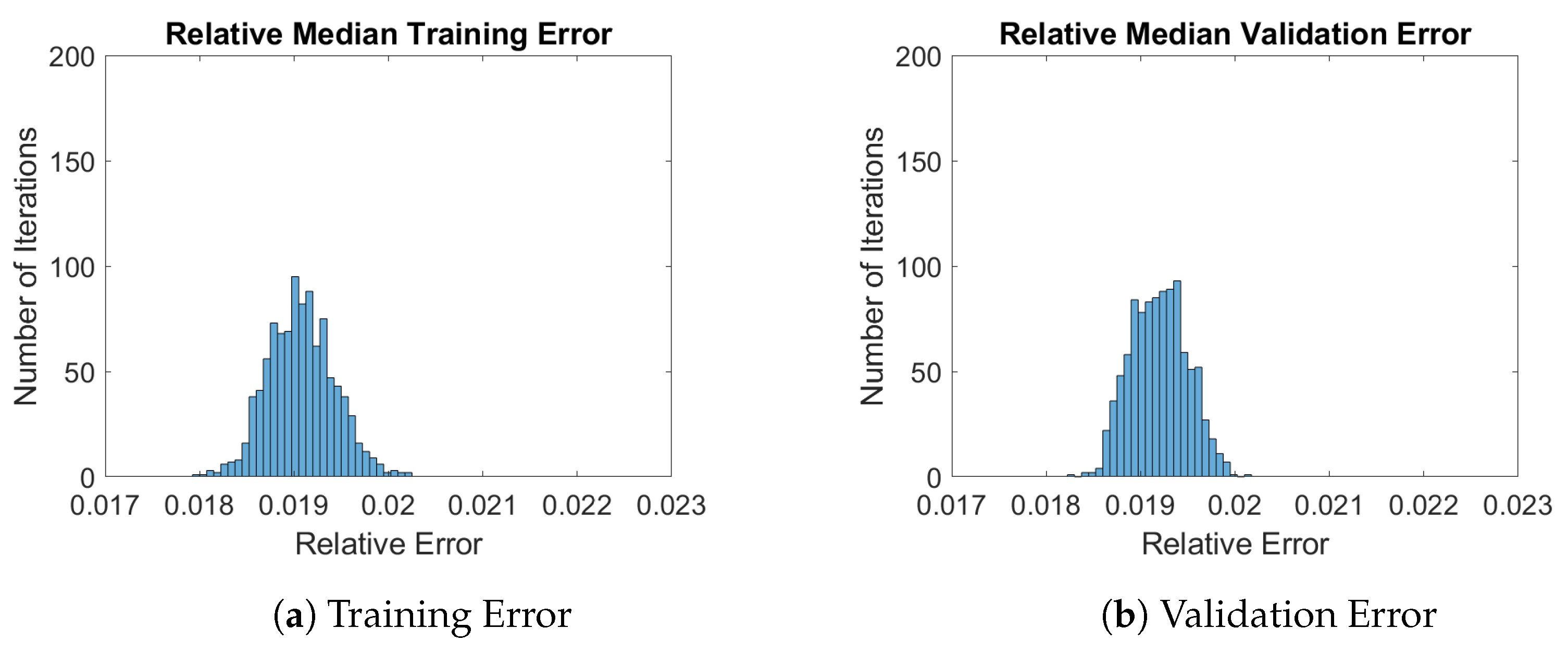
4.3. Implementing the Surrogate Model

To create the surrogate model, the 13 components that were created as part of the MOR process were collected into a 13 × 3600 matrix $\mathit{S}$, with each of the 3600 cases represented by its corresponding set of 13 components. A training set and validation set were created by randomly assigning half of the cases to each category, with 1800 cases in each. Various types and classes of surrogate models were tried. It was determined that a step-wise linear regression could be used to fit each of the 13 components as a function of the 6 input variables in Table 1, resulting in the creation of 13 surrogate models that could map each of the components to the inputs.

When components are predicted using the surrogate model, Equation (8) can be used to generate the predicted noise grid using the predicted components ${\mathit{S}}^{\prime }$ instead of $\mathit{S}$. The same basis vectors $\mathit{U}$ and mean value $\overline{w}$ obtained during the MOR step are used.

To ensure that the selected model is appropriate for the task, the model fitting process was repeated 1000 times, using random allocations for training and validation in each iteration. Each iteration of the model was evaluated to generate the corresponding predicted noise grid, which was then compared to the projected noise grid to determine model prediction error. The model fitting process, conducted over 1000 repetitions, took a total of 6 h. This results in an average of approximately 21.6 s per repetition.

The error within the surrogate modeling process was further sub-categorized as either a training error or a validation error. The training error was the error resulting from the 1800 cases that were used to train the model. The validation error was the error that was computed by deploying the model on input cases that were not used to train the model. This was done to check the applicability of the surrogate model to previously unseen data. The corresponding prediction errors for the training and validation data were then aggregated for analysis. The mean and median errors of each iteration were retained and are plotted below in Figure 7 and Figure 8. The prediction error distributions are centered around a fairly low error value of roughly 2% for both the mean and median, with ranges between 1.7% and 2.3%. This is a fairly low and reasonable value. In addition, both errors resemble a normal distribution, which indicates minimal bias introduced by the sampling of training and validation cases. The results indicate that the model building process produced accurate models, and the accuracy of the model was not dependent on a specific choice of the split between training or validation data.

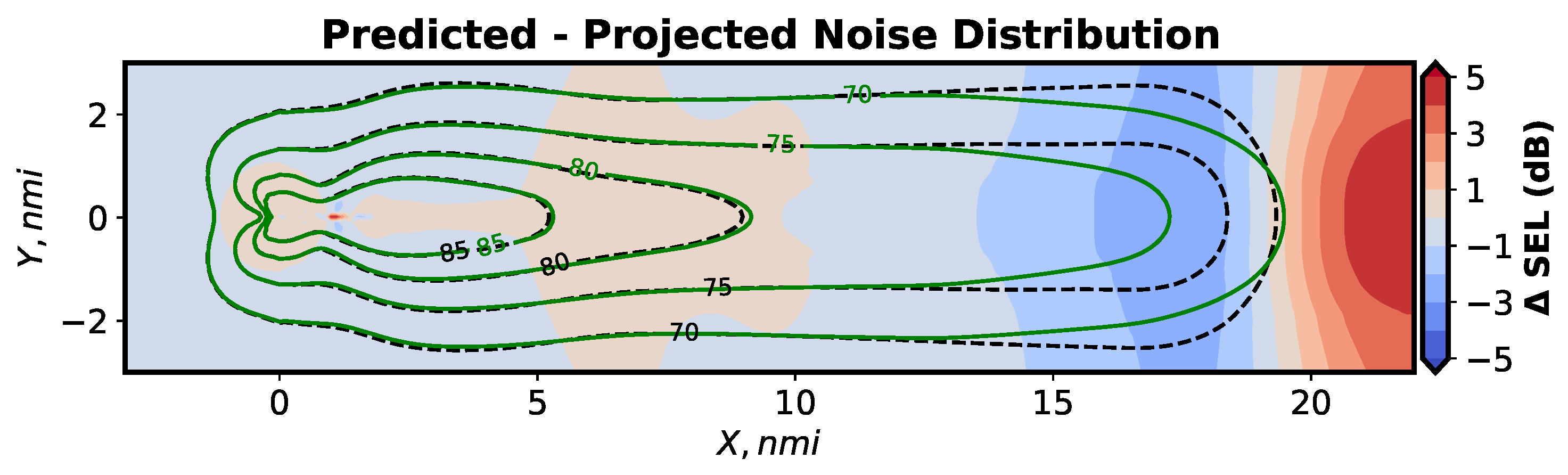
4.4. Total Error and Noise Grid Comparisons

The final model was evaluated not only in terms of its relative prediction errors but also by comparing across the entire noise grid to determine the effectiveness of the methodology at each grid point individually. For the methodology to be effective, the noise result of the predicted grid must resemble the actual grid across all receptors in the grid.

First, the difference between the predicted noise grid from the final model and the projected noise grid is determined at each receptor in the noise grid. This is the difference between the predicted and projected noise grid at each point, rather than a single relative error value representing the divergence across the entire grid. From the histogram of the relative difference shown in Figure 9, the majority of the points for the predicted noise have a difference of around 1%. While some locations have differences of up to 4.5%, these locations represent only a small fraction of the total number of points in the grid.

These differences are also determined between the predicted and original unprojected noise grids. The resulting differences, as shown in Figure 10, are found to be very similar to the differences from the projected noise grids, with similar distribution. This result is expected as the magnitude of the projection error was much lower than the magnitude of the prediction error. As a result, the major source of the actual error and, thus, the actual differences at each point, is from the surrogate model prediction.

To visualize the capability of the methodology in making predictions across the noise grid, Figure 11, Figure 12 and Figure 13 illustrate a comparison between the noise grid for the case with median total relative error. This case has the median total error from among the 3600 cases generated from the surrogate model. In all three comparisons, a heatmap of the SEL dB difference at each point in the noise grid is shown. The axes are centered in such a way that the origin is on the runway end where the start of the takeoff ground roll occurs. The departure track is along the positive X direction. Areas in red indicate regions of over-prediction by the methodology whereas areas in blue indicate regions of under-prediction. The predicted and original noise contours are overlaid in green and black, respectively.

Figure 11 showcases the difference between the projected and original noise grids for the specific case. Previously, it was found that there was little difference between the projected and actual noise grids during the MOR process, and the heatmap reflects this result, as there is essentially zero difference across the vast majority of the noise grid. Figure 12 depicts the difference between the predicted and projected noise grids, which indicates the error due to the creation of the surrogate model. It can be seen here that there is a larger difference than what is seen in Figure 11, with the surrogate model predicting slightly higher noise in the area between $X=5$ and $X=10$ nautical miles. In addition, the area between 15 and 20 nmi in the horizontal axis is underestimated to a small degree by the surrogate model. Notably, there is a more significant area of overestimation by the surrogate model at the very edge of the noise grid. This indicates that at faraway locations, the surrogate model struggles to make accurate predictions. However, it is important to note that the vast majority of the noise grid, including all areas close to the airport, shows little difference between the prediction and projection. In addition, the noise levels of 80 dB SEL and above were accurately recreated by the surrogate models.

Figure 13, showcasing the difference between the predicted and original noise grids, shows similar trends as Figure 12, albeit with minor differences in the shape of the heatmap. This was to be expected due to the previous finding that the magnitude of projection error compared to the magnitude of prediction error was much lower.

The prediction results from the 3600 input cases depicted in Table 1 are used to compute absolute errors relative to the original noise grid of the corresponding cases. The error values at each point are then aggregated across the 3600 cases into the mean absolute errors from projection and prediction, as shown in Figure 14. The mean errors are found to be within $\pm 0.05$ SEL dB across the grid. The result indicates that the methodology is able to accurately generate noise grids across the ranges of input parameters. However, a mean under-prediction of up to $-0.05$ SEL dB is observed from 15–18 nmi along the X direction of the noise grid.

To further explore the model’s accuracy in predicting the various SEL dB levels at different receptors in the grid, Figure 15 and Figure 16 illustrate the predicted vs. original plots, comparing the results of the final model to the corresponding original model. The predicted and original SEL dB values from each individual receptor are plotted for the 3600 cases. The results are subdivided into intervals based on the X distance from the start of takeoff.

Across all the cases, the model performs extremely well for noise close to the airport, as shown in Figure 15. The predicted and actual comparisons were found to be quite accurate within the first 10 nmi of the X distance. The results between 0 nmi and 5 nmi indicate highly accurate predictions below 90 SEL dB and slight variations in accuracy for noise levels between 90 SEL dB and 130 SEL dB. However, noise above 90 SEL dB is typically only seen at the start of takeoff and the contour containing 90+ SEL dB is generally limited to the airport boundary. Lower accuracy is seen further away from the start of the ground roll, specifically beyond 10 nmi, as shown in Figure 16. A tendency to over-predict is seen for noise below 70 SEL dB at distances between 10 nmi to 15 nmi.

Further decrease in accuracy is observed beyond 15 nmi. This result correlates with the error distributions seen in Figure 14. At these distances, the parameter input variations result in large variations in aircraft performance and noise propagation as compared to regions closer to the start of takeoff. To improve the model’s accuracy in these locations, additional combinations of thrust, acceleration altitude, energy share percentage, and weight can potentially be modeled, which would result in a more dense distribution of height AGL at 15 nmi ground track distance and beyond. In particular, raising the terminal altitude of these procedural profiles beyond 10,000 ft may also help with the accuracy in this region of the noise grid. The error in dB across the entire noise grid of 15,311 receptor points, and across all 3600 cases, is summarized in

Table 3. Summary of statistics for SEL dB differences across all cases.

Count	$15,311\times 3600=55,119,600$
Mean Difference	$-0.01$ SEL dB
Standard Deviation	$1.71$ SEL dB
Minimum Difference	$-16.33$ SEL dB
5%	$-2.67$ SEL dB
25%	$-0.42$ SEL dB
50%	$0.00$ SEL dB
75%	$0.43$ SEL dB
95%	$2.63$ SEL dB
Maximum Difference	$13.33$ SEL dB

. The minimum and maximum differences have high magnitudes due to being outlier values. Regardless, the methodology is able to predict noise behavior relatively well across the entire grid and range of noise levels. Incorporating additional input cases that capture variability further away could potentially improve the model’s accuracy.

5. Summary and Conclusions

A methodology for creating a rapid aviation noise model that maps relevant departure operation parameters to the SEL noise metric was created in this research. A set of six parameters were used as the inputs, consisting of the internal and controllable variables of altitude of acceleration, thrust reduction level, and energy share percentage, as well as the external and uncontrollable variables of aircraft weight, airport elevation, and temperature. The Aviation Environment Design Tool (AEDT) was used as the baseline model to obtain noise results for 3600 flight cases. Model order reduction was used to reduce the dimensionality of the noise results from 15,311 SEL values per noise grid to 13 components along 13 principal axes. This dimensionality reduction was performed using the principal component analysis and greatly reduced the number of variables needed to describe different noise grids. A surrogate model for each of the components was generated using step-wise regression, mapping the components to the input parameters.

The accuracy of the process was confirmed through analysis of the error introduced at each step of the process. It was found that the projection error was quite small, less than half a percent across the breadth of the cases, while the prediction error was larger, averaging at around 2%. The predicted noise grids were found to also be fairly accurate compared to the actual noise grids. The accuracy was observed to reduce further away from the airport, where regions of lower noise levels were observed in departure operations. The prediction step using surrogate models was found to be the main source of error within the process and could be improved with future work by including additional cases that capture variations in aircraft performance and noise propagation further from the airport.

This methodology can be deployed at any airport by characterizing its elevation and temperature conditions. However, it should be noted that the method cannot account for terrain effects, so a pre-requisite of using this model at any airport is that there should not be significant terrain height changes in the surroundings of the airport.

The methodology developed in this research lays the foundation for multi-query applications, such as parametric trade-off analyses and optimization studies. The developed rapid noise model can be used as a basis for future work in the optimization of noise abatement departure procedures. With the inclusion of airport and aircraft parameters, this model enables the development of frameworks, which optimize piloting actions for noise mitigation on the ground while also accounting for airport conditions, such as temperature and airport elevation. The addition of curved ground tracks in the model development would add an additional degree of freedom in minimizing noise impacts at desired locations.

References

1. Federal Aviation Administration. FAA Aerospace Forecast: 2022–2042. 2022. Available online: https://www.faa.gov/sites/faa.gov/files/2022-06/FY2022_42_FAA_Aerospace_Forecast.pdf (accessed on 14 May 2023).
2. Boeing. Commercial Market Outlook: 2022–2041. 2022. Available online: https://www.boeing.com/commercial/market/commercial-market-outlook/index.page (accessed on 14 May 2023).
3. Airbus. Global Market Forecast: 2022–2041. 2022. Available online: https://www.airbus.com/en/products-services/commercial-aircraft/market/global-market-forecast (accessed on 14 May 2023).
4. Zellmann, C.; Schäffer, B.; Wunderli, J.M.; Isermann, U.; Paschereit, C.O. Aircraft Noise Emission Model Accounting for Aircraft Flight Parameters. J. Aircr. 2018, 55, 682–695. [Google Scholar] [CrossRef]
5. Putnam, T.W. Review of Aircraft Noise Propagation; Technical Memorandum NASA TM X-56033; NASA Flight Research Center: Edwards, CA, USA, 1975. Available online: https://www.nasa.gov/centers/dryden/pdf/87865main_H-895.pdf (accessed on 14 May 2023).
6. Morrell, S.; Taylor, R.; Lyle, D. A review of health effects of aircraft noise. Aust. N. Z. J. Public Health 1997, 21, 221–236. [Google Scholar] [CrossRef] [PubMed]
7. Federal Aviation Administration. The FAA Airport Noise Program. 2015. Available online: https://www.faa.gov/newsroom/faa-airport-noise-program (accessed on 14 May 2023).
8. Federal Aviation Administration. FAA History of Noise. 2022. Available online: https://www.faa.gov/regulations_policies/policy_guidance/noise/history (accessed on 14 May 2023).
9. Erkelens, L. Research into new noise abatement procedures for the 21st century. In Proceedings of the AIAA Guidance, Navigation, and Control Conference and Exhibit, Dever, CO, USA, 4–17 August 2000. [Google Scholar] [CrossRef]
10. Lim, D.; Behere, A.; Jin, Y.C.D.; Li, Y.; Kirby, M.; Gao, Z.; Mavris, D.N. Improved Noise Abatement Departure Procedure Modeling for Aviation Environmental Impact Assessment. In Proceedings of the AIAA Scitech 2020 Forum, Orlando, FL, USA, 6–10 January 2020. [Google Scholar] [CrossRef]
11. Behere, A.; Lim, D.; Li, Y.; Jin, Y.C.D.; Gao, Z.; Kirby, M.; Mavris, D.N. Sensitivity Analysis of Airport level Environmental Impacts to Aircraft thrust, weight, and departure procedures. In Proceedings of the AIAA Scitech 2020 Forum, Orlando, FL, USA, 6–10 January 2020. [Google Scholar] [CrossRef]
12. Oruc, R.; Baklacioglu, T. Modeling of aircraft performance parameters with metaheuristic methods to achieve specific excess power contours using energy maneuverability method. Energy 2022, 259, 125069. [Google Scholar] [CrossRef]
13. McRae, M.; Lee, R.A.; Steinschneider, S.; Galgano, F. Assessing Aircraft Performance in a Warming Climate. Weather Clim. Soc. 2021, 13, 39–55. [Google Scholar] [CrossRef]
14. Huber, J.; Barringto, J.P. Three dimensional atmospheric propagation module for noise prediction. In Proceedings of the 40th AIAA Aerospace Sciences Meeting & Exhibit, Reno, NV, USA, 14–17 January 2002. [Google Scholar] [CrossRef]
15. Behere, A.; Mavris, D.N. Optimization of Takeoff Departure Procedures for Airport Noise Mitigation. Transp. Res. Rec. 2021, 2675, 81–92. [Google Scholar] [CrossRef]
16. Behere, A.R. A Reduced Order Modeling Methodology for the Parametric Estimation and Optimization of Aviation Noise. Ph.D. Thesis, Georgia Institute of Technology, Atlanta, GA, USA, 2022. [Google Scholar]
17. Behere, A.; Kirby, M.; Mavris, D.N. Relative Importance of Parameters in Departure Procedure Design for LTO Noise, Emission, and Fuel Burn Minimization. In Proceedings of the AIAA AVIATION 2022 Forum, Chicago, IL, USA, 27 June–1 July 2022. [Google Scholar] [CrossRef]
18. Aviation Environmental Design Tool (AEDT) Version 3e User Manual; User Manual; U.S. Department of Transportation Federal Aviation Administration: Washington, DC, USA, 2022.
19. Aviation Environmental Design Tool (AEDT) Version 3e Technical Manual; Technical Manual; U.S. Department of Transportation Federal Aviation Administration: Washington, DC, USA, 2022.
20. Behere, A.; Bhanpato, J.; Puranik, T.G.; Kirby, M.; Mavris, D.N. Data-driven Approach to Environmental Impact Assessment of Real-World Operations. In Proceedings of the AIAA Scitech 2021 Forum, Virtual, 11–15 January 2021. [Google Scholar] [CrossRef]
21. Bernardo, J.E. Formulation and Implementation of a Generic Fleet-Level Noise Methodology. Ph.D. Thesis, Georgia Institute of Technology, Atlanta, GA, USA, 2013. [Google Scholar]
22. LeVine, M.J.; Bernardo, J.E.; Kirby, M.; Mavris, D.N. Average Generic Vehicle Method for Fleet-Level Analysis of Noise and Emission Tradeoffs. J. Aircr. 2018, 55, 929–946. [Google Scholar] [CrossRef]
23. Zanella, P. Sensitivity Analysis for Noise and Emissions Based on Parametric Tracks. In Proceedings of the 17th AIAA Aviation Technology, Integration, and Operations Conference, Denver, CO, USA, 5–9 June 2017. [Google Scholar] [CrossRef]
24. LeVine, M.J.; Kaul, A.; Bernardo, J.E.; Kirby, M.; Mavris, D.N. Methodology for Calibration of ANGIM Subjected to Atmospheric Uncertainties. In Proceedings of the 2013 Aviation Technology, Integration, and Operations Conference, Los Angeles, CA, USA, 12–14 August 2013. [Google Scholar] [CrossRef]
25. Bertram, A.; Othmer, C.; Zimmermann, R. Towards Real-time Vehicle Aerodynamic Design via Multi-fidelity Data-driven Reduced Order Modeling. In Proceedings of the 2018 AIAA/ASCE/AHS/ASC Structures, Structural Dynamics, and Materials Conference, Kissimmee, FL, USA, 8–12 January 2018. [Google Scholar] [CrossRef]
26. Gogu, C. Improving the efficiency of large scale topology optimization through on-the-fly reduced order model construction. Int. J. Numer. Methods Eng. 2015, 101, 281–304. [Google Scholar] [CrossRef]
27. Fossati, M. Evaluation of Aerodynamic Loads via Reduced-Order Methodology. AIAA J. 2015, 53, 2389–2405. [Google Scholar] [CrossRef]
28. Mainini, L.; Willcox, K. Surrogate Modeling Approach to Support Real-Time Structural Assessment and Decision Making. AIAA J. 2015, 53, 1612–1626. [Google Scholar] [CrossRef]
29. Amsallem, D.; Cortial, J.; Farhat, C. Towards Real-Time Computational-Fluid-Dynamics-Based Aeroelastic Computations Using a Database of Reduced-Order Information. AIAA J. 2010, 48, 2029–2037. [Google Scholar] [CrossRef]
30. Behere, A.; Rajaram, D.; Puranik, T.G.; Kirby, M.; Mavris, D.N. Reduced Order Modeling Methods for Aviation Noise Estimation. Sustainability 2021, 13, 1120. [Google Scholar] [CrossRef]
31. Behere, A.; Mavris, D.N. Principal Component Analysis of Aviation Noise Grids for Dimensionality Reduction. In Proceedings of the AIAA SCITECH 2023 Forum, National Harbor, MD, USA, 23–27 January 2023. [Google Scholar] [CrossRef]
32. Benner, P.; Ohlberger, M.; Cohen, A.; Willcox, K. Model Reduction and Approximation; Society for Industrial and Applied Mathematics: Philadelphia, PA, USA, 2017. [Google Scholar] [CrossRef] [Green Version]
Figure 1. Outline of the overall methodology with model reduction and surrogate modeling.
Aerospace 10 00627 g001
Figure 2. Visualization of the projected and predicted noise grid snapshots, and their associated errors.
Aerospace 10 00627 g002
Figure 3. Relative information content obtained from increasing numbers of components.
Aerospace 10 00627 g003
Figure 4. Distribution of the relative error due to the projection for each case.
Aerospace 10 00627 g004
Figure 5. Distribution of projection error with respect to the internal inputs.
Aerospace 10 00627 g005
Figure 6. Distribution of projection error with respect to the external inputs.
Aerospace 10 00627 g006
Figure 7. Mean prediction errors.
Aerospace 10 00627 g007
Figure 8. Median prediction errors.
Aerospace 10 00627 g008
Figure 9. Relative differences at points in the noise grid between the predicted and projected noise grids.
Aerospace 10 00627 g009
Figure 10. Relative differences at points in the noise grid between the predicted and actual noise grids.
Aerospace 10 00627 g010
Figure 11. Sample differences between a set of projected and actual noise grids. Δ SEL = projected (green) − Actual (black).
Aerospace 10 00627 g011
Figure 12. Sample differences between a set of predicted and projected noise grids. Δ SEL = predicted (green) − projected (black).
Aerospace 10 00627 g012
Figure 13. Sample differences between a set of predicted and actual noise grids. Δ SEL = predicted (green) − actual (black).
Aerospace 10 00627 g013
Figure 14. Mean actual error across the noise grid. Δ SEL = predicted − actual.
Aerospace 10 00627 g014
Figure 15. Predicted v. actual plots, up to 10 nautical miles from the start of takeoff.
Aerospace 10 00627 g015
Figure 16. Predicted v. actual plots beyond 10 nautical miles from the start of takeoff.
Aerospace 10 00627 g016