Article

Micro- and Nanosatellite Sensorless Electromagnetic Docking Control Based on the High-Frequency Injection Method

1
College of Electrical Engineering, Zhejiang University, Hangzhou 310012, China
2
Beijing Institute of Spacecraft System Engineering, Beijing 100094, China
*
Author to whom correspondence should be addressed.
Aerospace 2023, 10(6), 547; https://doi.org/10.3390/aerospace10060547
Submission received: 21 March 2023 / Revised: 1 June 2023 / Accepted: 2 June 2023 / Published: 7 June 2023
(This article belongs to the Section Aeronautics)

Abstract

:
This paper proposes a sensorless electromagnetic docking method suitable for micro- and nanosatellites. Based on the circuit model of the electromagnetic docking device, an algorithm for calculating the distance between two satellites on the basis of the high-frequency injection (HFI) method has been developed. In the specific implementation, first, a high-frequency (HF) voltage is injected into one of the two electromagnets; second, the HF currents induced by both electromagnets are measured and their respective root-mean-squares (RMSs) are calculated; third, two RMSs are substituted into a specific formula to obtain a variable carrying distance information; finally, the variable is utilized to calculate the distance estimation using the look-up table interpolation method. This paper presents a closed-loop electromagnetic docking controller which includes an outer distance loop and an inner speed loop and adopts the distance estimation as the feedback. The proposed sensorless electromagnetic docking method is verified by the distance estimation tracking response test and the ground-based docking test. The results indicate that low-impact docking can be achieved under the initial condition that the two satellites have a certain degree of misalignment. The proposed method can be adopted as a primary or as a redundant electromagnetic docking solution for resource-critical micro- and nanosatellites.

1. Introduction

Because of the distinct advantages of low cost, light weight, and mass production, an increasing number of micro- and nanosatellites have been implemented in multi-agent space missions such as on-orbit servicing, in-orbit assembly, swarm-based construction, and reconfiguration [1]. On the other hand, due to the reduced volume of micro- and nanosatellites, small-sized sensors and actuators, which have few options available, have to be used, resulting in performance limitations. It has been reported that the most successful proximity operation CubeSat missions, CanX-4 and CanX-5, can only achieve centimeter-level position determination and sub-meter-level control accuracy [2]. Micro- and nanosatellite missions tend to involve multiple docking and undocking procedures. If traditional docking technology is utilized, a sub-meter level of accuracy will result in a significant docking impact and could lead to dock failure or even collision [3]. Hence, electromagnetic docking, which has been demonstrated in [4] to be able to achieve centimeter-level control accuracy and 1 mm/s final relative velocity through ground-based tests, has a promising application prospect in micro- and nanosatellites docking as one of the weak impact methods. Compared with traditional thruster-based docking, electromagnetic docking boasts many distinct advantages, such as low docking impact, no propellant consumption and plume contamination, and high-precision control capability including continuous, reversible, synchronous, and noncontact interaction. In addition, due to the overall reduced capability of micro- and nanosatellites in terms of power generation, computing, pose determination, and control, the rethinking of how to apply an electromagnetic docking system on them has turned into a challenge and an interesting problem from both research and engineering points of view.
The concept of electromagnetic docking was proposed around 2000. For more than 20 years, many scholars and research institutions have carried out abundant principle scheme explorations and experimental verification studies [5,6,7,8]. For example, NASA proposed the Mini AERCam mission and jointly developed LIDS, OASIS, and EGADS missions in cooperation with ESA, Washington State University, and the University of Texas, respectively. All these missions have performed the ground-based docking test on 1 degree-of-freedom (DOF) or 2DOF spacecraft simulators. It is worth mentioning that there are also a few missions that have undergone on-orbit verification. For instance, the SPHERES mission led by the Massachusetts Institute of Technology successfully completed the autonomous docking test onboard the International Space Station. Some missions are still in progress and scheduled for testing in space, such as the AAREST mission led by Caltech and the Surrey Space Center and the STRaND 2 mission led by the Surrey Space Center. The missions mentioned above have obtained remarkable achievements, but they typically employed hard docks to ensure dock completion. In [4], Rebecca C. Foust et al. proposed an ultra-soft electromagnetic docking system and performed ground-based docking tests on a fleet of 3DOF spacecraft simulators [9], demonstrating the excellent performance of electromagnetic docking. In that system, the electromagnet is used to regulate the distance, the reaction wheel is used to compensate for heading error, and the pose and the angular velocity for each spacecraft are determined by the motion capture system in the flat floor facility and the on-board gyroscope. Many studies have focused on the control methods to overcome the issues of model uncertainty, unknown external disturbances, and nonlinearity. Typically, Zhang et al. systematically designed an electromagnetic docking controller by using linear extended state observer, feedback linearization, and robust H control technology and verified the performance of the controller in simulation [10]. Electromagnetic docking has also been studied for the applications of formation flight applications [11,12] and contact-free docking [13,14,15]. In addition, the key feature of electromagnetic docking is the use of non-contact electromagnetic force and torque, which are also extended to some prospective applications such as a contactless technique for active debris removal [16], the rescue of a satellite with attitude fault [17], and attitude control of separated payload in fractionated spacecraft architecture [18].
In existing studies, the electromagnet is utilized as an actuator, and the relative distance between two satellites is determined by special sensors such as a laser distance sensor and motion camera. This increases the cost and weight of the satellite and occupies internal space and computing resources, resulting in high technical difficulties, especially in the application of micro- and nanosatellites. On the other hand, EMI will inevitably occur when the electromagnet is energized. For system safety reasons, under some specific circumstances, other components have to enter sleep mode when the electromagnetic docking device is operating. Therefore, if the electrical signal generated by the electromagnets while working can be adopted to estimate the relative distance as a feedback signal for docking, it will greatly reduce the cost and complexity of the satellite and improve its reliability. A mission-specific satellite then only needs to be equipped with the electromagnetic docking device and its associated mechanics, in addition to the necessary mission tools. In applications where sensors must be installed, it can also be used as an alternative to increase system redundancy in the event of a sensor failure.
This paper proposes a sensorless electromagnetic docking system based on the HFI method [19]. In Section 2, the voltage equations of the two-satellite electromagnet circuit model are transformed to obtain two independent resistor–inductance circuit voltage equations, through which a sensorless method for estimating the distance based on the HFI method is proposed. Section 3 describes a specially designed iron-core electromagnet for increasing the electromagnetic force, and a docking port for compensating for the limited attitude correction ability of the electromagnet, which is designed as a taper hole–taper rod coordination mechanism to restrict the non-docking axial movement so that the docking is carried out under the electromechanical cooperation. In Section 4, a closed-loop distance controller is designed using the distance estimation as the feedback, and an engineering treatment is given for the nonlinearity of the electromagnetic force. Section 5 presents the results of distance estimation tracking response tests and 3DOF ground-based docking tests conducted to verify the feasibility of the proposed sensorless electromagnetic docking system. In the end, conclusions are drawn in Section 6.

2. Sensorless Distance Estimation Method

In this section, the circuit of the electromagnetic docking system is analyzed, and its voltage equation is introduced. Through mathematical transformation and approximate treatment, the voltage equation is converted to two simple and independent inertial systems. Based on the fact that an inertial system has phase–frequency (PF) and amplitude–frequency (AF) characteristics in frequency domain, two distance estimation methods are proposed using these two characteristics, respectively.

2.1. Voltage Equation Transformation

Each electromagnet has its self-inductance, and there is a mutual inductance between the two electromagnets. The circuit diagram is shown in Figure 1. In this paper, the two satellites are called the target and the chaser, respectively.
The voltage equation of the system circuit can be expressed as
{ u T = R T i T + d L T ( d ) i T d t + d M ( d ) i C d t u C = R C i C + d L C ( d ) i C d t + d M ( d ) i T d t
where uT and uC are the terminal voltages of the electromagnets of the target and chaser, respectively; iT and iC are the currents; RT and RC are the resistances; LT and LC are the self-inductances; M is the mutual inductance; and d is the coil-to-coil distance, which is taken as the distance between the surface centers of the two electromagnets in this paper. The inductance is the ratio of the flux linkage to the excitation current, and the flux linkage is related to the magnetic induction intensity, which in turn is determined by the relative permeability of the medium. When the relative position and relative attitude of the two electromagnets change, the flux linkage generated by one electromagnet in the other electromagnet changes, causing a variation in mutual inductance; and due to the presence of the iron core (high relative permeability), the self-inductance also varies with the change in the relative permeability distribution in the free space. In summary, LT, LC, and M all vary with the coil-to-coil pose. For simplification, by assuming that the two electromagnets are aligned axially, the self-inductance and mutual inductance can be expressed as functions of distance: LT(d), LC(d), and M(d). When the currents are input into the electromagnets, the circuit depicted in Figure 1 is closed because the magnetic induction always exists no matter what the relative pose is. The circuit is similar to the equivalent circuit of a transformer [20], except that the main conduction path of the magnetic field lines changes from silicon steel sheets to free space.
The two electromagnets are of the same design. If the manufacturing error is ignored, the resistance and self-inductance of the two electromagnets are the same. Equation (1) can be simplified as
{ u T = R i T + d L ( d ) i T d t + d M ( d ) i C d t u C = R i C + d L ( d ) i C d t + d M ( d ) i T d t
where R is the resistance and L(d) is the self-inductance.
By transforming Equation (2), the following equation can be obtained:
{ u C u T = R ( i C i T ) + d [ L ( d ) M ( d ) ] ( i C i T ) d t u C + u T = R ( i C + i T ) + d [ L ( d ) + M ( d ) ] ( i C + i T ) d t
Set
{ u 1 = u C u T u 2 = u C + u T i 1 = i C i T i 2 = i C + i T L 1 ( d ) = L ( d ) M ( d ) L 2 ( d ) = L ( d ) + M ( d )
Substituting Equation (4) into Equation (3), we obtain
{ u 1 = R i 1 + L 1 ( d ) d i 1 d t + i 1 d L 1 ( d ) d d d d d t u 2 = R i 2 + L 2 ( d ) d i 2 d t + i 2 d L 2 ( d ) d d d d d t
where dd/dt term on the right side of the equation is the time derivative of the coil-to-coil distance d, which in the physical sense is the coil-to-coil speed. Considering that the two satellites are manipulated at a slow speed for docking, the third term on the right side of the equation can be neglected. It is obtained that
{ u 1 = R i 1 + L 1 ( d ) d i 1 d t u 2 = R i 2 + L 2 ( d ) d i 2 d t .
Therefore, the voltage equations shown in Equation (2) are simplified to the two independent resistor–inductance (R-L) circuit voltage equations shown in Equation (6). u1 and u2 are the terminal voltages of the simplified circuit 1 and circuit 2, respectively; i1 and i2 are the currents; and L1(d) and L2(d) are the self-inductances.
An HF voltage is injected into circuit 1 and circuit 2 shown in Equation (6), expressed as
{ u 1 = U HFI sin ( ω t + θ 0 ) u 2 = U HFI sin ( ω t + θ 0 )
where UHFI, ω, and θ0 are the amplitude, angular frequency, and initial angle of the injected HF voltage, respectively. This can also be expressed as the terminal voltage form of the two electromagnets:
{ u T = 0 u C = U HFI sin ( ω t + θ 0 ) .
This shows that only the chaser electromagnet is injected with the HF voltage. So, there is no synchronization issue.
Circuit 1 and circuit 2 are two simple inertial systems. After injection, the phase–frequency or amplitude–frequency characteristics of the two circuits can be used to estimate d. The methods are as follows.

2.2. Estimation Method Based on PF Characteristic

According to the property of inertia link, the PF characteristics of the system shown in Equation (6) can be expressed as
{ G 1 ( j ω ) = arctan ω T 1 G 2 ( j ω ) = arctan ω T 2
where
{ T 1 = L 1 ( d ) R T 2 = L 2 ( d ) R
where ∠G1() and ∠G2() are the phase angles of the circuit 1 and circuit 2 inertia system, respectively, and T1 and T2 are the time constants.
The phase angle difference between the induced current and the injected voltage is measured to obtain ∠G1() and ∠G2(), and then the self-inductances L1(d) and L2(d) can be calculated using the following equations:
{ L 1 ( d ) = tan G 1 ( j ω ) ω R L 2 ( d ) = tan G 2 ( j ω ) ω R
where L1(d) and L2(d) contain the information of d. In order to estimate d and reduce the influence of parameters as much as possible, a variable h is introduced:
h = L 2 ( d ) L 1 ( d ) = tan G 2 ( j ω ) tan G 1 ( j ω )
where h is the ratio of the inductances of circuit 2 and circuit 1, and it is continuous and monotonous as a function of d. Therefore, we can measure ∠G1() and ∠G2() and calculate h by using Equation (12), and then d can be estimated by querying the pre-calibrated h-d curve.

2.3. Estimation Method Based on AF Characteristic

According to the property of inertia link, the AF characteristics of the system shown in Equation (6) can be expressed as
{ | G 1 ( j ω ) | = 1 R 1 + ω 2 T 1 2 | G 2 ( j ω ) | = 1 R 1 + ω 2 T 2 2
where |G1()| and |G2()| are the amplitude ratios of the circuit 1 and circuit 2 inertia systems, respectively, which contain the information of d. In order to estimate d and reduce the influence of parameters as much as possible, a variable k is introduced:
k = | G 1 ( j ω ) | | G 2 ( j ω ) | = I 2 I 1 = R 2 + ω 2 L 2 ( d ) 2 R 2 + ω 2 L 1 ( d ) 2
where I1 and I2 are the RMSs of the induced currents of circuit 1 and circuit 2, respectively. k represents the RMS ratio of the induced currents of circuit 1 and circuit 2.
It can be seen from Equation (14) that if ω is large enough, R can be neglected so that the influence of resistance error caused by measurement and resistance change caused by coil heating can be avoided. Equation (14) can be rewritten as
k = L 2 ( d ) L 1 ( d ) = L ( d ) + M ( d ) L ( d ) M ( d )
where k is continuous and monotonous as a function of d. Therefore, we can measure I1 and I2 and calculate k by using Equation (15), and then d can be estimated by querying the pre-calibrated k-d curve. I1 and I2 can be calculated using the following equations:
{ I 1 = I C I T I 2 = I C + I T
where IT and IC are the RMSs of the induced currents of the target and chaser electromagnet respectively.
Two estimation methods are discussed above. In practice, because the two satellites are independent of each other, the data need to be transmitted via wireless signal (WIFI) which has a random time delay. However, the amount of data that needs to be transmitted for phase detection is large and the real-time requirement is high, so phase detection tools such as phase-locked loops cannot be used. In addition, the phase difference of the two inertial systems, circuit 1 and circuit 2, is very close (<5°) in the entire docking range, which will cause a large error in calculating h, so the PF characteristic estimation method is not applicable. In comparison, the AF characteristic estimation method does not require strict real-time data transmission. In the fastest case, it only needs to transmit the RMS of the induced current once per cycle. Furthermore, measuring the RMS can reduce the impact of white noise interference, so that the measurement accuracy is improved. Thus, this paper adopts the AF characteristic method to estimate the distance. It should be noted that when the communication rate is fast enough and the mutual inductance to self-inductance ratio is large enough, the PF characteristic method can be chosen and can update the distance estimation faster (which can be updated for each transmission) than the AF characteristic method.

3. Actuator Mechanism
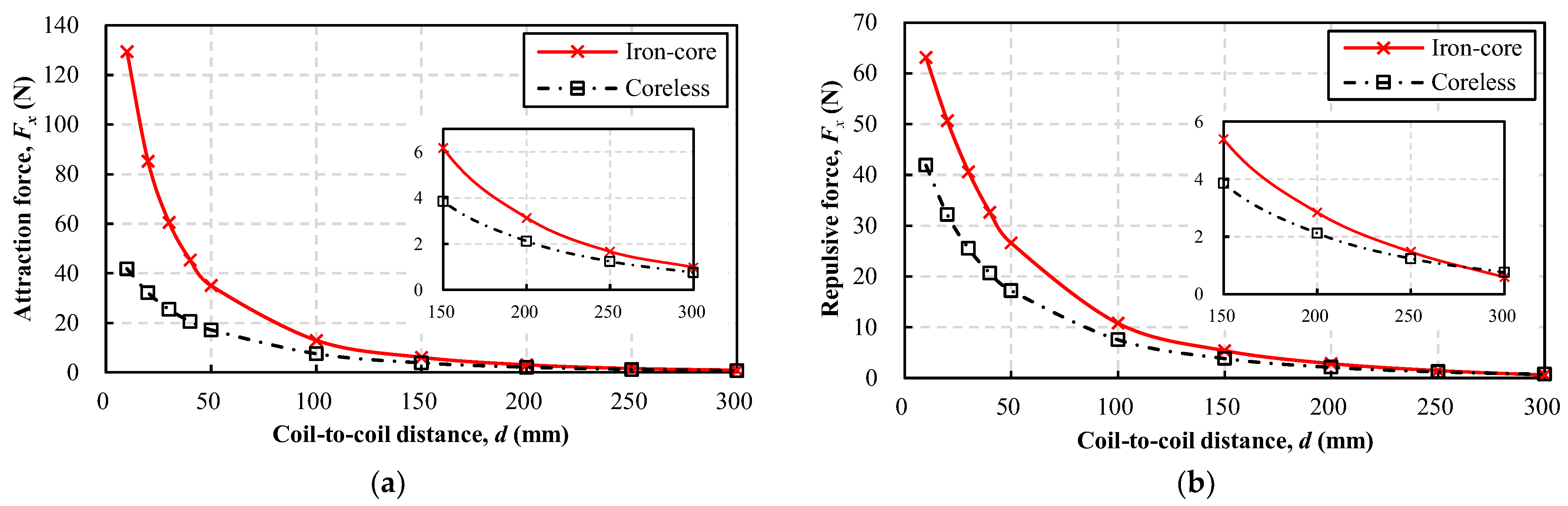
The actuator mechanism proposed in this paper mainly consists of two parts: electromagnet and docking port. The electromagnet is used to generate electromagnetic force, and the docking port is used to passively assist the electromagnet in attitude correction.

3.1. Electromagnet

A coreless electromagnet is adopted as an actuator in most of the existing studies because it possesses an exact electromagnetic force model, which is convenient for theoretical analysis and control algorithm design. However, under the same weight, power consumption, and distance, it provides a much weaker force than an iron-core electromagnet. In order to obtain a greater electromagnetic force to improve the docking efficiency, an iron-core electromagnet of the configuration shown in Figure 2 was utilized, with the dimensions and main parameters shown in Table 1. The iron-core material is a permalloy model 1J50, which has better magnetic focusing performance and less coercivity than ordinary iron-core materials, such as silicon steel.
Figure 3 shows the comparison of the electromagnetic force with and without the iron core. In the comparison test, the two electromagnets were coaxial, and each electromagnet was energized with 13.81 A current, which was the maximum current at which magnetic saturation did not occur in the iron core at a distance of 300 mm. It can be seen from the figure that the electromagnetic force was greatly enhanced by the addition of the iron core, especially the attraction force. At 300 mm, the attraction force was 0.98 N for the iron-core electromagnet and 0.75 N for the coreless electromagnet, which is also a significant improvement of a 31% increase. It should be noted that the repulsive force decreased at 300 mm: 0.59 N for the iron-core electromagnet and 0.75 N for the coreless electromagnet. This is because the iron-core C(T) is magnetized by coil T and coil C, respectively, and the coil T(C) part always generates an attraction force. When the distance is large, the coil T(C) proportion becomes larger, causing a decrease in repulsion compared to a coreless electromagnet. In general, the iron-core electromagnet, after reasonable optimization, can always have better attraction force output efficiency than the coreless electromagnet with the same mass due to the magnetic congregate effect brought by the iron core. The repulsive force output efficiency is also improved in the medium to short distance, but decreases when the distance is large.
To observe the influence of the added iron cores more intuitively, finite element simulations were conducted on the models of the iron-core electromagnet and coreless electromagnet. Figure 4 shows the comparison of the distribution of flux lines when two electromagnets are axially aligned at 100 mm and the full power current is applied to output attraction force. It can be seen that the iron core plays a role in providing the magnetic circuit, enhancing and guiding the magnetic flux, thereby increasing the force.

3.2. Docking Port

The electromagnet is equipped on the surface of the satellite and the mass center of the satellite is inside the body. If the two electromagnets are slightly misaligned, when they are generating attraction force, a side force reducing the misalignment and a torque correcting the heading error will occur [21]; otherwise, the opposite will happen. At the beginning of docking, the electromagnets are unlikely to be aligned axially, and the relative speed and angular velocity of the satellites are uncertain. If the docking only relies on the electromagnets, the allowable range of the initial state of the satellites will be very narrow, and once exceeded, the docking will fail or even a collision may take place. In order to improve the tolerance and avoid docking failure, the taper hole–taper rod coordination mechanism as shown in Figure 5 is proposed, which is installed on the fixture and fastened with the coil and the iron core as a whole. The docking is, thus, carried out in the form of electromechanical cooperation. In this study, the taper hole and the taper rod of the electromagnetic docking system for ground-based test were made of nylon. When actually used in space, they need to be made of metal or special materials to resist cosmic rays.
As shown in Figure 6, the docking port mechanism divides the docking process into four stages, as follows:
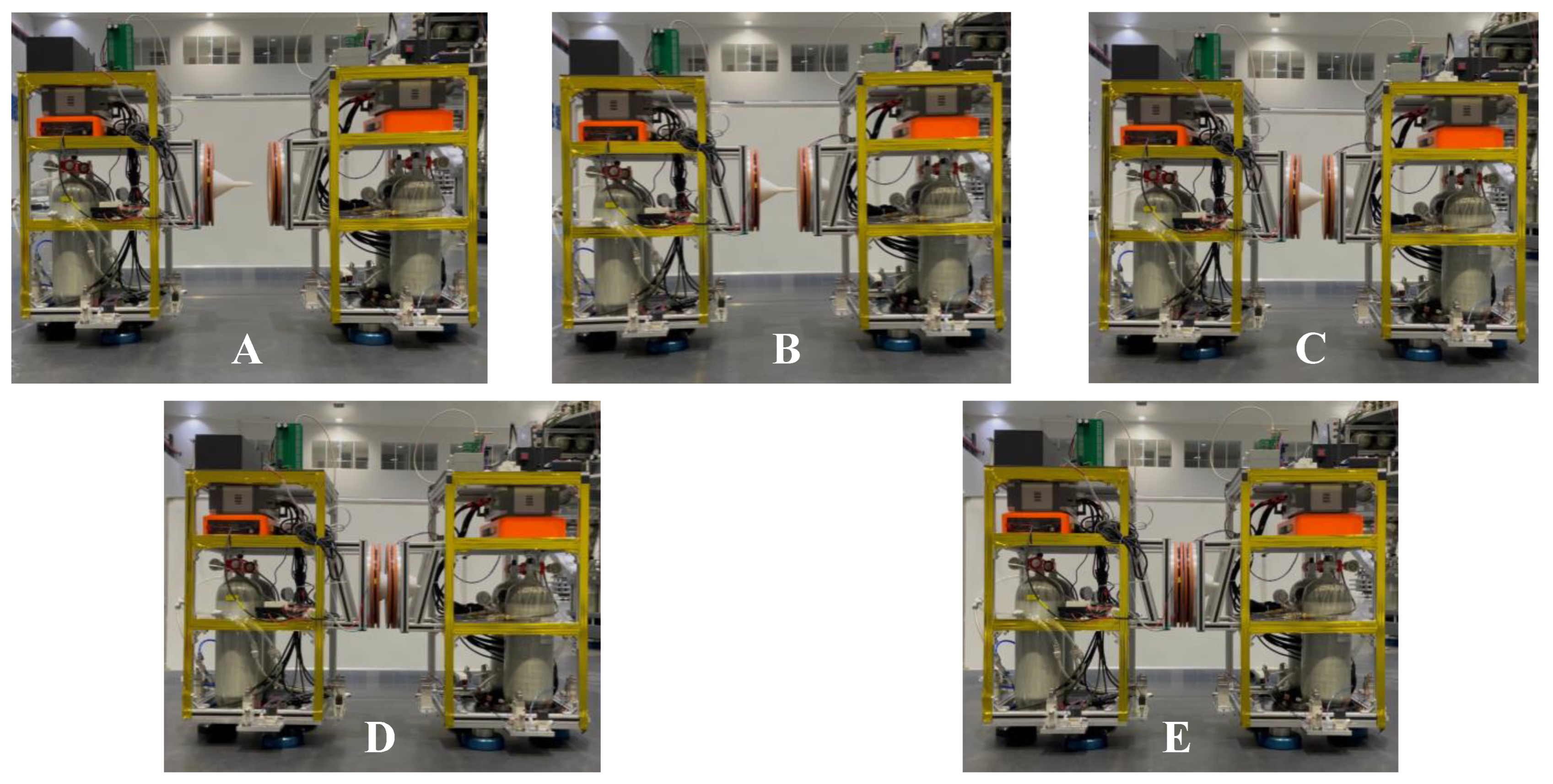
  • Non-touching Docking Stage. The two satellites are not in contact during this stage, and they are brought closer from a distance at a limited speed.
  • Aligning Stage. At this stage, the front end of the taper rod enters the enveloping cone of the taper hole for the first time. If there is a large misalignment, the taper rod will lightly collide with the surface of the taper hole and be ejected. The electromagnetic docking control system then pulls the two satellites closer again, and the misalignment and the heading error continue to be reduced. The process of collision and pulling will be repeated several times until the front end of the taper rod passes through the funnel mouth of the rod hole, at which point the two satellites are basically aligned. Note that there is no active orientation using an actuator such as a momentum wheel, and the aligning is passively accomplished by attraction force.
  • Touching Docking Stage. When the front end crosses through the funnel mouth, the chaser will not escape, and the two satellites will continue to be smoothly pulled closer. At this time, there will be a small friction due to the contact between the taper rod and the taper hole.
  • Locking Stage. At this stage, the docking process is completed, and finally, a large attraction force is output using the electromagnets to squeeze the locking mechanism so that the two satellites are locked and fixed.

4. Control Strategy

The designed control algorithm runs in the two-satellite driver MCUs. The electromagnet is driven by H-bridge, and the switching frequency is 10 kHz. The current is sampled by using a low-tolerance shunt resistor to ensure linearity, and the sampling frequency is fspl = 10 kHz. The closed-loop control system has been developed based on the following main points:

4.1. Task Allocation

The target driver’s task is to output a fixed voltage UDC to its electromagnet, measure IT, and wirelessly transmit IT to the chaser driver at a regular frequency ftx. The chaser driver is the main control unit, which runs the distance estimation algorithm and the motion control algorithm. The chaser driver measures IC and substitutes it with the received IT into Equations (14) and (16) to obtain k. Then, d is estimated by querying the k-d curve. By using d as the feedback, the control loop computes and outputs the control voltage uC for the electromagnet.
Such task allocation will make the power consumption mainly concentrated on the target driver, but the control logic becomes simple and clear. Because the electromagnetic force is an internal force, the tasks of the chaser and the target driver can be interchanged, and this does not have an impact on the motion control.

4.2. Frequency and Amplitude of the Injected Voltage

In the selection of the injection frequency fHFI, the following aspects need to be considered: Firstly, in the control process, the injection voltage and the control voltage are added and output to the electromagnet, so in order to avoid mutual interference between the control loop and the distance estimation, fHFI must be greater than the control frequency fctrl. Secondly, for increasing the calculation accuracy of the current RMS, fHFI should be sufficiently less than fspl to increase the number of current samples per cycle (generally more than 24). Thirdly, fHFI should be as high as possible when the first two aspects are satisfied, because the induced current will additionally generate a sinusoidal electromagnetic force that will lead to a speed ripple, yet the higher the frequency, the smaller the ripple.
On the premise of ensuring a high signal-to-noise ratio for the estimation, the amplitude UHFI should be as small as possible to reduce the occupation of the DC link voltage and lower the power drain.
This paper sets UHFI = 15 V and fHFI = 200 Hz. The related test performance and results refer to the experimental results part of this paper.

4.3. RMS Calculation

After the sampled current is bandpass filtered, the RMS of the frequency fHFI current is the next to be computed. The calculation formula can be expressed as
I RMS = n = 0 M 1 i 2 ( n ) M
where i(n) is a sampled current and M is the number of samples per cycle. In this paper, fspl = 10 kHz and fHFI = 200 Hz, so we have M = 50.

4.4. k-d Curve

Because of the nonlinearity brought by the iron core and the fact that the docking is chosen to start at a relatively close distance (the docking range is limited to 300 mm, which is only 1.0 times the electromagnet radius, while 6–8 radii are required for an electromagnetic coil to be accurately equivalent to a magnetic dipole [22]) in this paper, the k-d curve does not have an accurate analytical solution. Thus, the experimental calibration method was used to obtain the k-d curve. Normally, the calibrated k-d curve can be curve-fitted to a formula. However, the formula is very complicated and needs a long computing time to obtain a result when running in the MCU as a program. Instead, the look-up table interpolation method is used for calculation. The calibrated k-d curve can be found in Section 5.2.1.

4.5. Control Loop

The whole closed-loop control system contains an outer-loop distance controller and an inner-loop speed controller. The control frequency is set to fctrl = ftx = 100 Hz, which is only 1/2 of fHFI, for making the estimation and control fully separated in the frequency domain to avoid mutual interference. In order to avoid the dynamic overshoot of the distance response, the distance loop simply adopts a P controller, takes d as input, and outputs a speed setpoint vd*. The speed loop uses a PI controller, takes vd* as input, and outputs a force setpoint F* that is limited to the upper and lower saturation values. The feedback speed vd for the speed loop is obtained by d differentiation. Since the speed is quite small, the back EMF in the electromagnet can be ignored compared to the resistance voltage. Therefore, for simplicity, the control voltage uctrl computed from F* is directly output for the electromagnet to obtain the required current. Therefore, the terminal voltages of the two electromagnets can be expressed as
{ u T = U DC u C = u ctrl + U HFI sin ( ω t + θ 0 ) .
The above can be transformed into the circuit 1 and circuit 2 form,
{ u 1 = U DC + u ctrl + U HFI sin ( ω t + θ 0 ) u 2 = U DC + u ctrl + U HFI sin ( ω t + θ 0 )
where UDC = 26 V, UHFI = 15 V, |uctrl| ≤ 26 V, and ω = 400 π in this paper. When the control loop outputs the maximum absolute value of uctrl, the chaser electromagnet works at full power.
Figure 7 visually displays the waveform diagrams of control variables including voltage, current, electromagnetic force, and speed. When the HF sinusoidal voltage uC (see Figure 7a) is injected, HF sinusoidal currents with different amplitudes and phases are generated in the two electromagnets accordingly (see Figure 7b). The force is proportional to the product of two currents, and its waveform is also sinusoidal (see Figure 7c). Due to the filtering effect of the mass integration link (m−1/s) on HF signals, the force can only cause a very small speed ripple. In Figure 7, the force with an amplitude of 0.7 N and a frequency of 200 Hz causes only a negligible speed ripple of 0.01 mm/s under a mass of 90 kg (see Figure 7d).

4.6. Electromagnetic Force Output Linearization

Since there is no analytical solution of uctrl computed from F*, and the relationship between F* and uctrl changes with distance, the experimental calibration method was also used to obtain the (F*, d)-uctrl curves. uctrl was calculated using the 2D look-up table interpolation method. The calibrated (F*, d)-uctrl curves can be found in Section 5.2.2.

4.7. Filter Parameters

In order to obtain the current of frequency fHFI, a bandpass filter is required to filter the sampled current. This paper adopts a discrete 2-order Butterworth bandpass filter with a center frequency of 200 Hz and a passband bandwidth of 10 Hz. It should be noted that too narrow a passband bandwidth will cause excessive delay, but too wide a passband bandwidth will weaken the noise suppression effect. In addition, two lowpass filters are used to suppress the noise of the estimated d and vd (speed, obtained by differentiating d), respectively. These lowpass filters adopt the discrete IIR filter, of which the pulse transfer function is
G LPF ( z ) = A 1 B z 1
where A and B are the parameters of the lowpass filter. The bandwidth of the lowpass filter for vd should not be set too narrow just to enhance the noise repression; otherwise, it will cause a signal lag and affect the control accuracy of the speed loop. On the other hand, because the speed loop adopts a PI controller, the integration link in it already has a certain suppression effect on the noise.

4.8. Trajectory Planner

Because there is no other signal to gain more information except for the currents of two electromagnets, the distance estimation is the only variable that can be fed into the control loop, and thus the trajectory is designed as a 1DOF scalar of distance. Fortunately, when the two electromagnets generate an attraction force, the pulling closer will always be accompanied by an adjustment of the relative attitude so that the two satellites can be aligned. Additionally, two docking ports are designed to cooperate with the electromagnets. If there is a misalignment between the two satellites, the two docking ports will collide and then bounce off (the relative velocity should be controlled during this process to make the collision very weak). Then, the attraction force will again pull close and passively align the two satellites. Therefore, with the electromechanical cooperation method, the docking can be completed by applying only the distance trajectory.
To avoid response overshoot and thus make the docking more flexible, a step function is not adopted as the distance reference. In this paper, the trajectory planner is implemented and divided into four parts in accordance with the docking port, as shown in Figure 8.
For Trajectory I, a ramp function is utilized as a reference trajectory. The distance setpoint decreases from d0* to d1* with a slope v1* = (d1* − d0*)/(t1* − t0*). d0* is initially assigned to the present value d, and d1* is set at a certain distance in the Touching Docking Stage. Because noise could be very high at long distances, the maximum distance estimation is saturated under 300 mm, which leads to d0* ≤ 300 mm, and the control parameters are also calibrated within that range. As described in Section 3.1, the electromagnets can provide a 0.98 N attraction force with full power at 300 mm, which means that if the distance can be accurately measured, the maximum effective distance can be longer.
For Trajectory II, the reference is kept as d1*. A positioning tolerance der1* is set. If |dd1*| ≤ der1* and is maintained for 2 s, then it is considered that docking to d1* has been completed, and the next trajectory starts. Otherwise, if it is not completed after 4 s, Trajectory I is restarted from the present position.
For Trajectory III, the reference trajectory is set to a ramp function again, the range of distance setpoint is from d1* to d2*, and the slope is v2* = (d2* − d1*)/(t2* − t1*). d2* is set at the point where the docking can finish or locking can be started.
For Trajectory IV, the reference is kept as d2*. A positioning tolerance der2* is set. If |dd2*| ≤ der2* and is maintained for 2 s, then it is considered that docking to d2* has been completed, and the closed-loop control ends.
In Trajectory I, the electromagnetic docking runs in the Non-touching Docking Stage or the Aligning Stage with a long docking stroke. In Trajectory III, it has entered the Touching Docking Stage, and only a short docking stroke has to be completed. Different filtering and control parameters are set for Trajectories I and II and Trajectories III and IV.

4.9. Control Block Diagram

In summary, the block diagram of sensorless electromagnetic docking control is shown in Figure 9.

5. Experimental Results

This section first analyzes the two induced currents to demonstrate the phenomenon of current change in the two electromagnets after HF voltage injection, so as to verify the rationality of using the HFI method to estimate the distance. Since the look-up table interpolation method is adopted to cope with the nonlinearity as well as to reduce the computational burden, calibrations are required. Therefore, the second subsection presents the calibrated data of the k-d curve and the (F, d)-uctrl curves, which are used in the control algorithm program. The third subsection verifies the effectiveness of the distance estimation algorithm by presenting the results of a tracking response test conducted on a static test bench. Finally, in the fourth subsection, the overall docking performance of the sensorless electromagnetic docking device is verified by the results of ground-based docking tests conducted after the distance estimation was fed into the control loop.

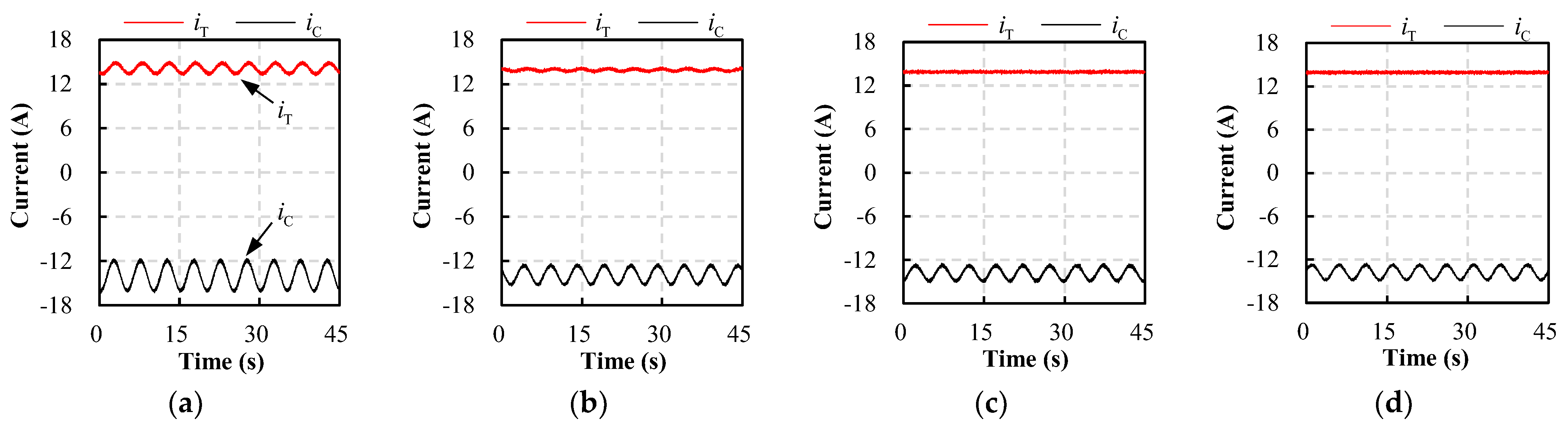
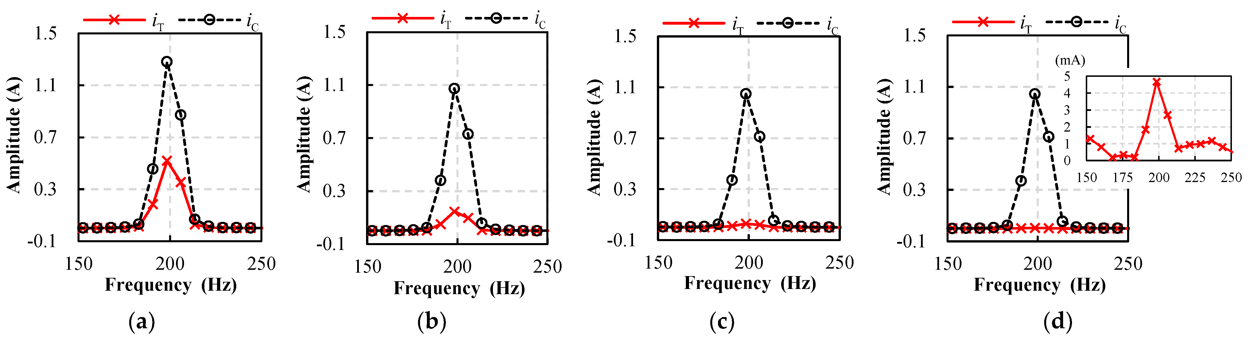
5.1. Induced Current Analysis

The static test bench shown in Figure 10 was made to test electromagnetic force, perform calibration, verify the distance estimation algorithm, etc. There is a force gauge on the bench to measure electromagnetic force and a laser distance sensor to measure the coil-to-coil axial distance. One electromagnet is fixed on the base, and the other is installed on a sliding plate, which can move axially and radially. The handle on the top of the bench is used to adjust the coil-to-coil axial distance, and several distance pieces of different sizes are processed and used to adjust the coil-to-coil radial distance. The radial sliding rail and the distance piece are used to adjust radial deviation, while the two electromagnets are still parallel.
First, the appropriate HFI voltage and fixed output voltage were determined through repeated trials on the bench, i.e., UDC = 26 V, UHFI = 15 V, fHFI = 200 Hz. The specific parameter determination process is not discussed in this paper. At four coil-to-coil axial distances of 10 mm, 50 mm, 150 mm, and 300 mm, the two electromagnets were energized with corresponding voltages, and their induced currents were observed. The specific test input conditions can be seen in Table 2.
The waveforms of the induced currents are shown in Figure 11. It can be seen that the closer the distance, the larger the induced HF current of the target electromagnet. When the distance is greater than 150 mm, the HF component can no longer be visually distinguished from the waveform. In addition, the induced HF current of the chaser electromagnet also decreases as the distance increases. These performances illustrate the feasibility of using AF characteristics to estimate distance. In order to make the comparison of the HF components clear, FFT analysis was carried out on the sampled currents, and the results are shown in Figure 12. The amplitude of the induced current of the target electromagnet at 300 mm cannot be seen clearly, so the waveform was enlarged, as shown in Figure 12d. This shows that at 300 mm, although the induced HF current component (5 mA) can be basically distinguished from the noise (about 2 mA), there will be some noise when measuring the RMS due to its small size. However, as the distance becomes shorter, the signal-to-noise ratio increases. In addition, it can be seen from Figure 11 that the phase angle difference of the two induced currents changes very little at different distances (due to the low ratio of mutual inductance to self-inductance), so the PF characteristics cannot be used to estimate distance in this study.

5.2. Calibration

5.2.1. k-d Curve

The calibration result of the k-d curve is shown in Figure 13. The closer the distance, the denser the calibration points. Since the two electromagnets are separated by the fixture, the nearest calibration distance is 9 mm.

5.2.2. (F*, d)-uctrl Curves

The calibration results of the (F*, d)-uctrl curves are shown in Figure 14. Seven sets of force, namely +3 N, +2 N, +1 N, 0 N, −1 N, −2 N, and −3 N, were calibrated, which can already meet the needs of electromagnetic docking. In this paper, F* is saturated as −1.5 N ≤ F* ≤ 1.5 N, and in order not to exceed the limit of power consumption, we set |uctrl| ≤ 26 V.

5.3. Distance Estimation Tracking Response Test

The distance estimation tracking response test was carried out on the static test bench, and the main control parameters are shown in Table 3. In this experiment, the two electromagnets were manually moved from a distance of 20 mm to approximately 250 mm and then moved back to about 20 mm. The estimated distance and the actual distance measured by the laser distance sensor were collected throughout the whole process, as shown in Figure 15. It can be seen from the curves that the estimated distance can follow the actual distance well, but due to the delay caused by the filters, wireless transmission, algorithm computing time, etc., the estimated distance lags about 0.1 s behind the actual distance. However, since the two satellites are manipulated to dock at a slow speed, the delay does not lay much negative impact on control. In addition, it can be seen that the estimation is considerably accurate when the two electromagnets are close, but a high level of noise occurs when the distance is beyond 200 mm. However, because the electromagnetic docking is in the Non-touching Docking Stage at this period, the noise will not bring a large docking impact. As the distance decreases, the control will become more precise.

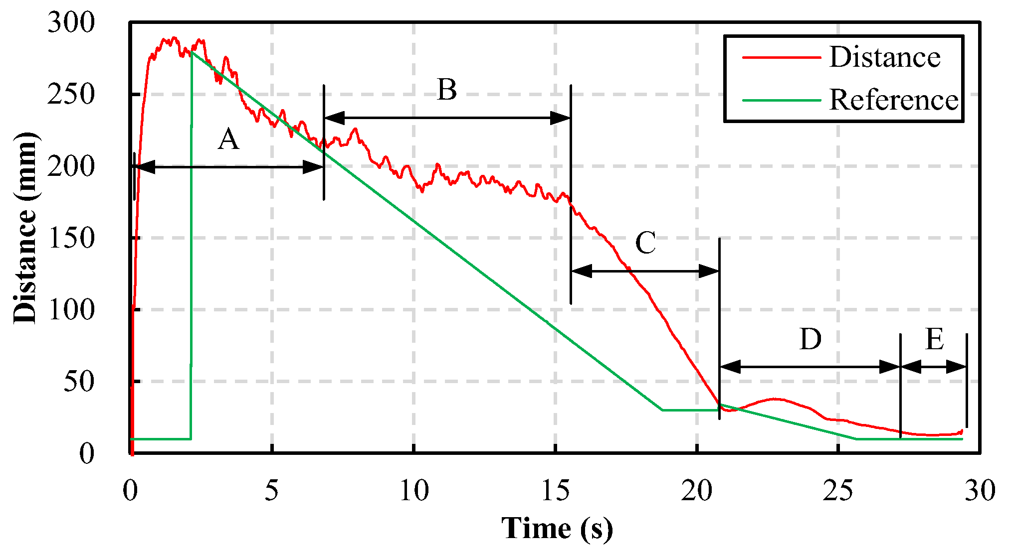
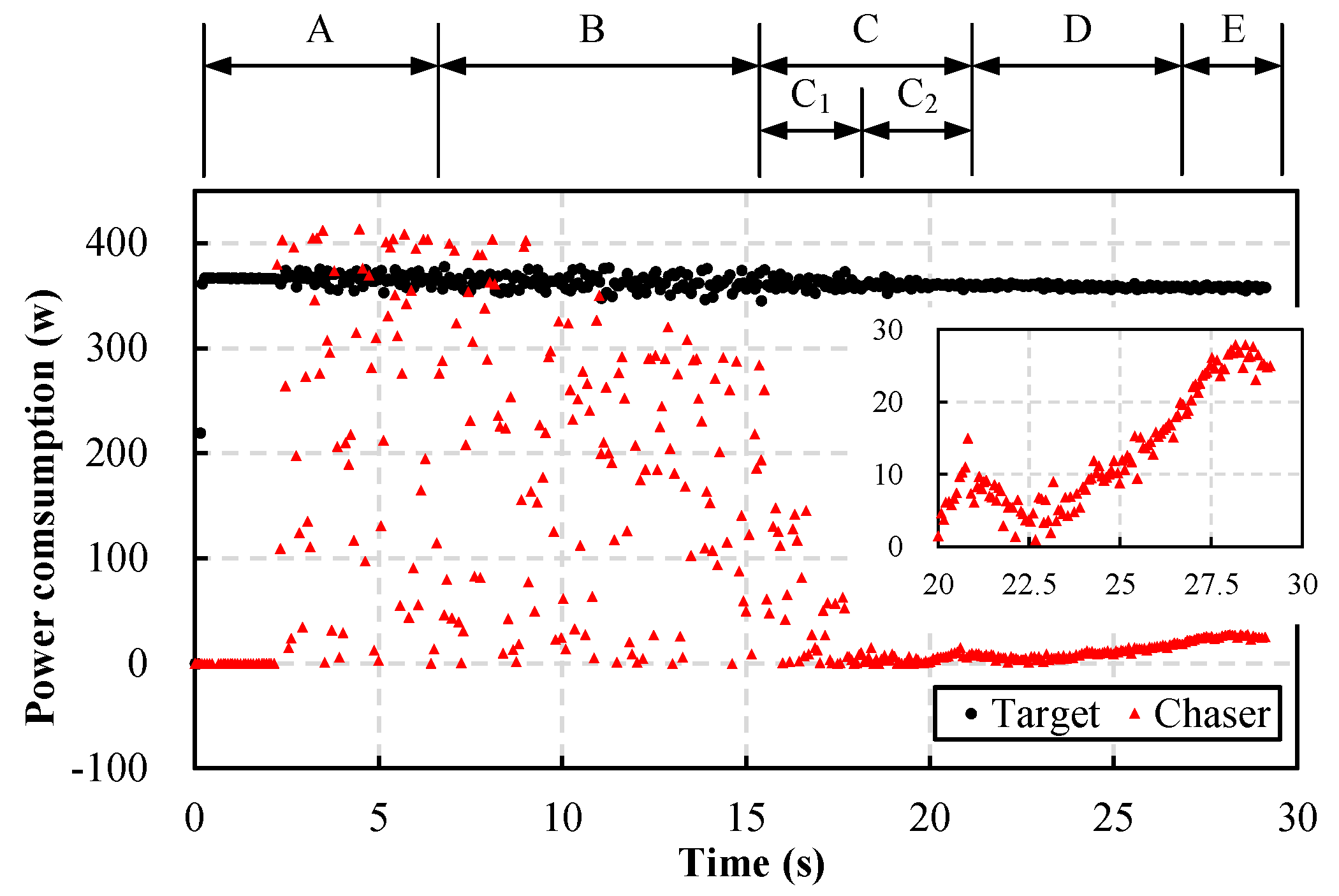
5.4. Ground-Based Docking Test

Two 3DOF (translation and yaw) spacecraft simulators were constructed for the docking test, as depicted in Figure 16. Both satellites have identical electromagnetic docking system hardware, mainly including the battery, driver, wireless AP repeater, electromagnet, and docking port. The key information is transmitted via WIFI, and the main control algorithm of the system runs on the microcontroller of the chaser. The satellite is also equipped with a thruster-based position and heading control system, the main components of which are a compressed air tank, electric valve, battery, driver, etc. The weight of each satellite is about 100 kg.
Experimental validation of the sensorless electromagnetic docking test was performed in a precision flat floor facility, as shown in Figure 16. The satellites were supported by the flat air bearings and floated on the floor. Due to the smooth surface and the well-designed facility, the friction between the floor and the flat air bearing was very small. The control parameters of the ground-based docking test are shown in Table 4. During the test, the chaser approached the target from a long distance by jet propulsion and tried to align with the target. When the coil-to-coil distance reached below 300 mm, the position and heading control system stopped working, and the sensorless electromagnetic docking system began to operate. At this point, there was a certain amount of misalignment between the two satellites due to the accuracy of the jet propulsion. It should be noted that the thrusters are only used to propel the chaser from a distance to the target, in order to simulate the actual docking situation as much as possible. When the distance reached the working range of the sensorless electromagnetic docking device, the thruster system stopped, and the control of the spacecraft was fully handed over to the electromagnetic docking device. The purpose of stopping the thruster system was to test the ability of the device to dock independently without the assistance of any other actuators and without position and attitude signals measured by sensors. One of the motivations for developing this device is for it to serve as a redundant solution for docking in case of damage to or absence of sensors such as motion cameras and IMUs and actuators such as momentum wheels. Throughout the docking process, the control variables such as trajectory reference, estimated distance, and output voltage were collected for analysis. Several tests were performed, and the result of one is shown in Figure 17. Time period A in the figure corresponds to Non-touching Docking Stage. At this period, due to the relatively low signal-to-noise ratio, there was some noise in distance estimation, but it was still able to track the reference. When the process ran to time period B, the docking entered the Aligning Stage. The taper rod bounced off the surface of the taper hole after slightly hitting it (so the error in relation to the reference trajectory became high), and then it pulled closer again. This process was repeated several times so that the misalignment was reduced. Trajectory I continued in time period B, and the trajectory reference and the distance presented a gradually increasing error. Running to time period C, the misalignment was basically removed, the taper rod began to gradually move towards the funnel mouth, and the error between the trajectory reference and the distance decreased rapidly. In addition, in time period C, Trajectory I ended and Trajectory II started to run, and as the distance decreased, the noise in the distance estimation became low. In time period D, the Touching Docking Stage was entered. After a brief adjustment at the funnel mouth, the front end of the taper rod started to advance steadily. During time period D, Trajectory III and Trajectory IV were executed successively. The final time period was time period E. After the tracking error was maintained within the positioning tolerance for more than 2 s, it was determined that the electromagnetic docking had been completed, and the Locking Stage was then started. Figure 18 shows the five periods A, B, C, D, and E. The link to the docking video can be found in Appendix A.
The force setpoint F* and the control voltage uctrl during the docking process can be seen in Figure 19. This figure shows that in the early stage of docking, due to the noise in the distance estimation, F* changed rapidly. When the distance decreased, especially in the Touching Docking Stage, due to the increased signal-to-noise ratio and the damping effect of friction, the range of F* change became smaller and the attraction force components appeared.
Figure 20 shows the instantaneous power consumption results obtained during the docking process. It can be seen that the power output by the chaser varied widely in the time periods A, B, and C1. This is because during these periods, the set force was rapidly adjusted, while the distance was relatively large, requiring a high current to obtain the desired force. During these periods, the power consumption of the target also oscillated due to the frequently varying current in the chaser electromagnet inducing the varying currents in the target electromagnet. When the C2 time period was entered, the distance had become small, making the estimation more accurate and the output efficiency of electromagnetic force higher. Thus, the power consumption of the chaser became stable and smaller. For the whole process, the mean power consumption was around 362 W for the target and 106 W for the chaser. In proximity, this metric for chaser was less than 30 W. In addition, the maximum instantaneous power of the chaser reached 414 W. The power supply and the electromagnet driver of the chaser need to meet this power level, and if it is scaled down, the docking duration will increase.
Out of the nine tests conducted on the flat floor, seven tests successfully docked and two did not dock due to the large initial misalignment caused by the thrusters. A trajectory overlay of all seven successful trials can be seen in Figure 21. It is observed that the changes in the initial entry state cause significant differences in trajectories. However, all seven trials show the same five periods as in Figure 17 (result of Test 1). Because of the limited amount of high-pressure gas (propulsion using thrusters is very gas-consuming, while supplying flat air bearings consumes less), the sensitivity to misalignment is not accurately measured. However, in the early debugging stage, some tests were conducted by manually setting the relative pose, and it was observed that a radial deviation of 50 mm and an angle error of within 10° could be tolerated under an initial distance of 300 mm.
The duration and the mean power consumption results of the seven sensorless docking tests are listed in Table 5. Combined with Figure 21, it can be seen that when the initial distance is farther, the overall docking duration will increase, as will the power consumption. If the docking starts with a close initial distance and minor initial misalignment, the energy loss will be greatly reduced, as in Test 4, where the mean power consumption of the chaser was only 9 W.
In summary, excluding the failures caused by excessive initial misalignments, the sensorless electromagnetic docking test based on the HFI method is successful.
It should be pointed out that it is also feasible to integrate the proposed system with a standard CubeSat. The spacecraft simulator designed in this paper weighs around 100 kg, and for the kilogram-level CubeSat, the required electromagnetic force is reduced. Thus, both the electromagnet and the docking port size can be decreased, and the corresponding power level will be reduced. In addition, most of the CubeSat communication systems operate in the VHF/UHF amateur frequency band with a data rate of 1.2 kbps and 9.6 kbps, and some have reached 1 Mbps or above [23]. The data transmission frequency used in this paper is 200 Hz, and only one current RMS datum needs to be transmitted each time. If a 12-bit resolution (a commonly used ADC sampling resolution of microcontrollers) is applied for these data, the communication between two satellites requires a data stream of 200 × 12 = 2.4 kbit per second, which is applicable to CubeSat communication.

6. Conclusions

This paper studies the sensorless control of electromagnetic docking. A distance estimation algorithm based on the HFI method is presented, and an engineered closed-loop docking control system is developed on the basis of this algorithm and related hardware. In this study, an iron-core electromagnet is utilized instead of a coreless electromagnet. Compared with a coreless electromagnet, the iron-core electromagnet can significantly increase the force under the condition of the same mass and power consumption. In addition, the docking port is designed in the form of a taper hole–taper rod fit to assist the attitude correction, which fixes the electromagnet inside and divides the entire electromagnetic docking process into four stages: Non-touching Docking, Aligning, Touching Docking, and Locking. Ground-based experiment results show that the HFI-based sensorless electromagnetic docking method proposed in this paper can achieve flexible docking under the initial condition that the two satellites have a certain extent of misalignment. Compared with traditional docking methods, the proposed docking method has the following advantages: sensors are not required to determine the distance; actuators such as reaction flywheels and thrusters are not required for orientation; only electrical energy is consumed and no plume pollution is generated in close proximity; a simple structure, for which only an electromagnet (docking port and electromagnet integrated together) and the corresponding driver (H-bridge) are required, which can be easily installed on micro- and nanosatellites; and a simple algorithm, for which only periodic transmission of current RMS information between the two satellites is required, which is a small computational burden for micro- and nanosatellites. In summary, the proposed docking system can independently complete docking tasks and is suitable for micro- and nanosatellites with stringent resource requirements.

Author Contributions

Conceptualization, L.W. and G.R.; Methodology, G.R.; Software, G.R.; Validation, G.R.; Formal Analysis, G.R.; Investigation, L.W. and G.R.; Resources, Y.W., B.W. and R.H.; Data Curation, G.R.; Writing—Original Draft Preparation, G.R.; Writing—Review and Editing, L.W., Y.W., B.W. and R.H.; Supervision, L.W. and Y.W.; Project Administration, B.W. and R.H. All authors have read and agreed to the published version of the manuscript.

Funding

This research received no external funding.

Data Availability Statement

Not applicable.

Acknowledgments

The authors acknowledge the Beijing Institute of Spacecraft System Engineering for providing topics, putting forward requirements, and granting project funding.

Conflicts of Interest

The authors declare no conflict of interest.

Appendix A. Experiment Video

HFI-based Sensorless Electromagnetic Docking Test Video: https://b23.tv/GU3dFI0 accessed on 9 March 2023.

References

  1. Bandyopadhyay, S.; Chung, S.-J.; Foust, R.; Subramanian, G. Review of formation flying and constellation missions using nanosatellites. J. Spacecr. Rockets 2016, 53, 567–578. [Google Scholar] [CrossRef] [Green Version]
  2. Bonin, G.; Roth, N.; Armitage, S.; Newman, J.; Risi, B.; Zee, R. CanX–4 and CanX–5 precision formation flight: Mission accomplished! In Proceedings of the 29th AIAA/USU Conference on Small Satellites, Logan, UT, USA, 11 August 2015; pp. 1–15. [Google Scholar]
  3. Bonometti, J. Boom rendezvous alternative docking approach. In Proceedings of the Space 2006 Conference, San Jose, CA, USA, 19–21 September 2006; pp. 1–13. [Google Scholar]
  4. Foust, R.C.; Lupu, E.S.; Nakka, Y.K.; Chung, S.-J.; Hadaegh, F.Y. Ultra-soft electromagnetic docking with applications to in-orbit assembly. In Proceedings of the 69th International Astronautical Congress (IAC), Bremen, Germany, 1–5 October 2018; pp. 1–14. [Google Scholar]
  5. Wang, B.; Zhuang, Y.; Liu, P.; Wang, N.; Han, R. Review of spacecraft electromagnetic docking technology development. Spacecr. Eng. 2018, 27, 92–101. [Google Scholar]
  6. Zhang, Y.W.; Yang, L.P.; Zhu, Y.W.; Huang, H.; Qi, D.W. Spacecraft electromagnetic docking: A review on dynamics and control. In Proceedings of the AIAA/AAS Astrodynamics Specialist Conference, San Diego, CA, USA, 4–7 August 2014; pp. 1–11. [Google Scholar]
  7. Shoer, J.; Wilson, W.; Jones, L.; Knobel, M.; Peck, M. Microgravity demonstrations of flux Pinning for station-keeping and reconfiguration of cubeSat-sized spacecraft. J. Spacecr. Rockets 2010, 47, 1066–1070. [Google Scholar] [CrossRef] [Green Version]
  8. Zhang, Y.W. Piece-wise control of constant electromagnetic moments for spacecraft self- and soft-docking exploiting dynamics conservation. Asian J. Control. 2021, 23, 2459–2473. [Google Scholar] [CrossRef]
  9. Nakka, Y.K.; Foust, R.C.; Lupu, E.S.; Elliott, D.B.; Crowell, I.S.; Chung, S.-J.; Hadaegh, F.Y. A six degree-of-freedom spacecraft dynamics simulator for formation control research. In Proceedings of the 2018 AAS/AIAA Astrodynamics Specialist Conference, Snowbird, UT, USA, 1 August 2018; pp. 1–20. [Google Scholar]
  10. Zhang, Y.W.; Yang, L.P.; Zhu, Y.W.; Huang, H.; Cai, W.W. Nonlinear 6-DOF control of spacecraft docking with inter-satellite electromagnetic force. Acta Astronaut. 2012, 77, 97–108. [Google Scholar] [CrossRef]
  11. Kong, E.; Kwon, D.W.; Schweighart, S.A.; Elias, L.M.; Sedwick, R.J.; Miller, D.W. Electromagnetic formation flight for multisatellite arrays. J. Spacecr. Rockets 2004, 41, 659–666. [Google Scholar] [CrossRef]
  12. Huang, H.; Cai, W.W.; Yang, L.P. 6-DOF formation keeping control for an invariant three-craft triangular electromagnetic formation. Adv. Space Res. 2020, 65, 312–325. [Google Scholar] [CrossRef]
  13. Jones, L.L.; Wilson, W.R.; Peck, M. Design parameters and validation for a non-contacting flux-pinned docking interface. In Proceedings of the AIAA SPACE 2010 Conference & Exposition, Anaheim, CA, USA, 30 August–2 September 2010; pp. 1–11. [Google Scholar]
  14. Zhu, F.; Dominguez, M.; Peck, M.; Jones, L. Flight-experiment validation of the dynamic capabilities of a flux-pinned interface as a docking mechanism. In Proceedings of the 2019 IEEE Aerospace Conference, Big Sky, MT, USA, 2–9 March 2019; pp. 1–13. [Google Scholar]
  15. Zhang, Y.W.; Yang, L.P.; Zhu, H.K. Spacecraft self- and soft-docking control approach with electromagnetic/magnetic flux-pinning synergy. In Proceedings of the 39th Chinese Control Conference, Shenyang, China, 27–29 July 2020; pp. 6721–6725. [Google Scholar]
  16. Voirin, T.; Kowaltschek, S.; Matra, O.D. NoMAD: A contactless technique for active large debris removal. In Proceedings of the 63rd International Astronautical Congress, Naples, Italy, 5 October 2012; pp. 1–14. [Google Scholar]
  17. Ao, H.J.; Yang, L.P.; Zhu, Y.W.; Zhang, Y.W.; Huang, H. Touchless attitude correction for satellite with constant magnetic moment. Adv. Space Res. 2017, 60, 915–924. [Google Scholar]
  18. Qin, Y.; Dong, W.B.; Zhao, L.P. Fractionated payload 3-DOF attitude control using only electromagnetic actuation. Aerosp. Sci. Technol. 2020, 107, 106237. [Google Scholar] [CrossRef]
  19. Wang, G.L.; Vella, M.; Solsona, J. Position sensorless permanent magnet synchronous machine drives—A review. IEEE Trans. Ind. Electr. 2020, 67, 5830–5842. [Google Scholar] [CrossRef]
  20. Fitzgerald, A.E.; Kingsley, C.; Umans, S.D. Electric Machinery, 6th ed.; McGraw-Hill: New York, NY, USA, 2003; p. 70. [Google Scholar]
  21. Duzzi, M.; Mazzucato, M.; Casagrande, R.; Moro, L.; Trevisi, F.; Vitellino, F.; Vitturi, M.; Cenedese, A.; Lorencini, E.C.; Francesconi, A. PACMAN Experiment: A CubeSat-size integrated system for proximity navigation and soft-docking. In Proceedings of the Small Satellite Systems and Services (4S Symposium), Sorrento, Italy, 1 June 2018; pp. 1–15. [Google Scholar]
  22. Schweighart, S.A. Electromagnetic Formation Flight Dipole Solution Planning. Ph.D. Thesis, Massachusetts Institute of Technology, Cambridge, MA, USA, 2005. [Google Scholar]
  23. Saeed, N.; Elzanaty, A.; Almorad, H.; Dahrouj, H.; Al-Naffouri, T.Y.; Alouini, M.S. CubeSat communications: Recent advances and future challenges. IEEE Commun. Surv. Tutor. 2020, 22, 1839–1862. [Google Scholar] [CrossRef]
Figure 1. Circuit diagram of electromagnetic docking device.
Aerospace 10 00547 g001
Figure 2. Electromagnet design. (a) Configuration of the electromagnet; (b) section of the electromagnet.
Aerospace 10 00547 g002
Figure 3. Comparison of electromagnetic force between iron-core electromagnet and coreless electromagnet. (a) Attraction force; (b) repulsive force.
Aerospace 10 00547 g003
Figure 4. Comparison of the distribution of flux lines between iron-core electromagnet and coreless electromagnet. (a) Iron core; (b) coreless.
Aerospace 10 00547 g004
Figure 5. Electromagnet assembly design.
Aerospace 10 00547 g005
Figure 6. Four Docking Stages. (a) Non-touching Docking Stage; (b) Aligning Stage; (c) Touching Docking Stage; (d) Locking Stage.
Aerospace 10 00547 g006
Figure 7. Waveform diagrams of control variables. (a) Voltages; (b) currents; (c) force; (d) speed ripple.
Aerospace 10 00547 g007
Figure 8. Schematic diagram of the proposed trajectory.
Aerospace 10 00547 g008
Figure 9. Block diagram of sensorless electromagnetic docking control.
Aerospace 10 00547 g009
Figure 10. Static test bench.
Aerospace 10 00547 g010
Figure 11. Comparison of induced currents at 4 different distances: (a) 10 mm; (b) 50 mm; (c) 150 mm; (d) 300 mm.
Aerospace 10 00547 g011
Figure 12. FFT analysis of induced currents at 4 different distances: (a) 10 mm; (b) 50 mm; (c) 150 mm; (d) 300 mm.
Aerospace 10 00547 g012
Figure 13. k-d curve.
Aerospace 10 00547 g013
Figure 14. (F*, d)-uctrl curves.
Aerospace 10 00547 g014
Figure 15. Distance estimation tracking response test.
Aerospace 10 00547 g015
Figure 16. Spacecraft simulator facility and two microsatellites with the two electromagnetic docking system.
Aerospace 10 00547 g016
Figure 17. Result of the sensorless electromagnetic docking control test.
Aerospace 10 00547 g017
Figure 18. Process of sensorless electromagnetic docking.
Aerospace 10 00547 g018
Figure 19. F* and uctrl vs. time.
Aerospace 10 00547 g019
Figure 20. Power consumption results.
Aerospace 10 00547 g020
Figure 21. Trajectory overlay of 7 successful trials.
Aerospace 10 00547 g021
Table 1. Dimensions and main parameters of the electromagnet.
DimensionsMain Parameters
D0300 mmSlot filling factor0.62
L045 mmWire diameterΦ1.5 mm
H013.72 mmNumber of turns216
Hc15.22 mmResistance1.9 Ω @ 45 °C
Tc1.5 mmInductance13.5 mH @ 100 Hz
3.0 mH @ 10 kHz
Maximum allowable current16.4 A @ 45 °C
Coil mass2.765 kg
Iron-core mass0.55 kg
Table 2. Test input conditions for induced current analysis.
The terminal voltage of chaser electromagnet, uC26.0 V @ DC, 15 V @ 200 Hz
The terminal voltage of target electromagnet, uT26.0 V @ DC
Coil-to-coil axial distance (mm)10, 50, 150, 300
Table 3. Control parameters of distance estimation tracking response test.
The fixed output voltage, UDC (V)26
The amplitude of the injected voltage, UHFI (V)15
The frequency of the injected voltage, fHFI (Hz)200
The upper frequency of the bandpass filter (Hz)205
The lower frequency of the bandpass filter (Hz)195
Parameter A of the distance lowpass filter0.1
Parameter B of the distance lowpass filter0.9
Table 4. Control parameters of ground-based docking test.
ParameterTrajectory I, IITrajectory III, IV
The fixed output voltage, UDC (V)2626
The amplitude of the injected voltage, UHFI (V)1515
The frequency of the injected voltage, fHFI (Hz)200200
The upper frequency of the bandpass filter (Hz)205205
The lower frequency of the bandpass filter (Hz)195195
Parameter A 1 of the distance lowpass filter0.10.1
Parameter B 1 of the distance lowpass filter0.90.9
Parameter A of the speed lowpass filter0.20.5
Parameter B of the speed lowpass filter0.80.5
Trajectory reference, d* (mm)d1* = 30d2* = 10
Positioning tolerance, der (mm)der1* = 5der2* = 5
Trajectory slope, v* (mm/s)v1* = 15v2* = 5
Parameter P of distance controller11
Upper limit of distance controller output (mm/s)3015
Lower limit of distance controller output (mm/s)−30−15
Parameter P of speed controller5050
Parameter I of speed controller0.10.1
Upper limit of speed controller output (N)1.51.5
Lower limit of speed controller output (N)−1.5−1.5
1 Parameters shown in Equation (20).
Table 5. Docking duration and mean power consumption results of 7 successful trials.
Test No.Docking Duration
(s)
Target
Power Consumption (w)
Chaser
Power Consumption (w)
Duration RankPower Rank
127.07362.44106.3567
224.53366.8041.8844
322.55372.0780.2725
421.42372.769.2911
530.33361.15104.3676
623.28366.1625.9332
725.4380.3536.3553
Disclaimer/Publisher’s Note: The statements, opinions and data contained in all publications are solely those of the individual author(s) and contributor(s) and not of MDPI and/or the editor(s). MDPI and/or the editor(s) disclaim responsibility for any injury to people or property resulting from any ideas, methods, instructions or products referred to in the content.

