Closed-Loop Control of Transonic Buffet Using Active Shock Control Bump

Abstract

At transonic flight conditions, the buffet caused by the shockwave/boundary-layer interaction can degrade aircraft performance and even threaten their safety. In this paper, a closed-loop control using an active shock control bump (SCB) has been proposed to suppress the buffet on a supercritical airfoil flying at transonic speeds. A closed-loop control law is designed by using the lift coefficient as the feedback signal and using the bump height as the control variable. The unsteady numerical simulations show that the buffet can be effectively suppressed by an optimal combination of the parameters of the control law, namely the gain and the delay time. Furthermore, the buffet control effectiveness is still acceptably constrained by a prescribed maximum bump height, which is believed to be practically important. In addition to being able to achieve both wave drag reduction and buffet alleviation, the active SCB is less sensitive to the parameters of the control law and has a shorter response time in comparison with the reference active trailing edge flap.

1. Introduction

The aerodynamic shape design of civil transport aircraft is strongly constrained by the transonic buffet boundary [1]. At high subsonic Mach numbers or high angles of attack, periodic shock motion with large amplitudes can be observed on the wings. That is because the interaction between the shock wave and the separated boundary layer results in a self-sustained periodic shock motion [2]. The related ongoing oscillating loads on aircraft may cause structural fatigue and even flight accidents, which severely limit the flight envelope of civil transport aircraft. Therefore, research on suppressing the transonic buffet is of practical significance for modern and future civil transport aircraft.

Transonic buffet involves complex shockwave/boundary-layer interactions that pose significant challenges to numerical simulations. Jacquin et al. [3] performed the buffet experiment on the OAT15A airfoil section in the ONERA S3Ch transonic wind tunnel and developed an extensive experimental database for the validation of numerical buffet simulations. It was found that the most promising approach was using high-fidelity Reynolds stress models and higher-order methods which can capture essential flow physics, such as detached-eddy simulations by Deck [4], Grossi et al. [5], Zhang et al. [6], and Huang et al. [7]. However, such techniques are currently not practical for exploring a large parameter space due to their extremely high computational cost. Levy [8] and Iovnovich [9] assessed the efficacy of various unsteady Reynolds-averaged Navier-Stokes (URANS) methods for capturing transonic buffets. Recently, Giannelis et al. [10,11] also performed a related transonic buffet simulation using the URANS method based on the k-$\omega$ SST turbulence model and obtained a good prediction of buffet frequency and shock oscillation amplitude.

The advancement of numerical methods in simulating the transonic buffet promoted a lot of research on controlling the shockwave/boundary-layer interaction through various control methods. Passive control methods such as streamwise slots [12,13], shock control bumps [14], and vortex generators [15,16], and active control methods such as trailing edge deflectors (TED) [17,18], fluidic vortex generators [19], and trailing edge flaps (TEF) [20], have been extensively studied. For instance, the trailing edge deflector was designed to change the airfoil trailing edge to achieve an effective buffet alleviation [18]. In particular, Caruana et al. [17,18] developed a trailing edge deflector with a closed-loop control to suppress the transonic buffet. Their study found that optimal control was achieved when the TED oscillation frequency was close to the buffet frequency. In addition, the trailing edge flap, considered a further development of TED, was also investigated by Gao et al. [20] and Ren et al. [21]. They demonstrated that a well-designed control law was crucial for effective buffet alleviation under various buffet conditions.

The passive shock control bumps (SCB) were also found to be able to delay the buffet boundary. In early studies [22,23,24], the application of SCBs mainly sought to reduce transonic pressure wave drag without the significant viscous drag penalty. In particular, Birkemeyer et al. [22] found that the shock control bumps positioned significantly downstream of the shock wave could reduce pressure fluctuations close to the trailing edge, thus delaying the shockwave/boundary-layer interaction. Later, Mayer et al. [25,26] compared and assessed two types of contour bumps for delaying buffet onset based on the URANS method. The results showed that besides delaying buffet onset by increasing the maximum lift coefficient, two-dimensional bumps were also capable of damping buffet-related lift oscillations in the buffet regime by an efficient shock strength reduction in combination with positive effects on flow separation. Tian et al. [27] found that the downstream SCB had better buffet performance over a range of freestream conditions and that the bump could weaken the downstream adverse pressure gradient as well as suppress the separation bubble at the shock foot merged with trailing edge separation. Geoghegan et al. [28,29,30] conducted a number of parametric studies on oscillating shock control bumps (open-loop control) for buffet alleviation. They found that the SCB location was an important parameter and should be placed between the shock wave and the trailing edge to suppress the buffet. The main drawback of passive bumps and oscillating bumps is that the optimal bump location for wave drag reduction is different from that for transonic buffet alleviation. Therefore, a trade-off design is needed to improve the overall mean and unsteady characteristics of an airfoil over a wide range of angles of attack [26].

Recently, it was found by Zhang et al. [31] that passive shock control bumps could effectively cooperate with the active trailing edge flap, providing both wave drag reduction and buffet alleviation. More importantly, it was found that buffet control assisted by a passive shock control bump was even more robust than the reference active trailing edge flap. Unlike the control device that relies on changing the flow dynamics near the trailing edge, shock control bumps can reduce shockwave strength, providing an alternative and possibly a more robust way to suppress the transonic buffet. The present paper reports further advances in reducing the complexity of the active buffet control system proposed in [31] by abandoning the active trailing edge flap. Instead, the bump height is assumed to be an active control variable according to the feedback signal, namely the lift coefficient. Note that a similar control method, named “local smart skin”, has been previously proposed by Ren et al. [32]. The current study will further extend their study on a well-understood buffet case and demonstrate the advantages of the active shock control bump in comparison with the reference active trailing edge flap. The proposed SCB-based control system shows more robust performances on buffet suppression over a wide range of flow conditions compared to the active TEF system.

The paper is organized as follows. Firstly, the active control devices and the corresponding closed-loop control law are introduced, followed by a validation of the numerical methods. Secondly, the active shock control bump driven by the feedback of the lift coefficient is investigated and the effects of parameters of the control law on buffet suppression are discussed. Finally, the advantages of the proposed buffet control method are demonstrated by comparing it with the reference active TEF, followed by the conclusions.

2. Problem Definition

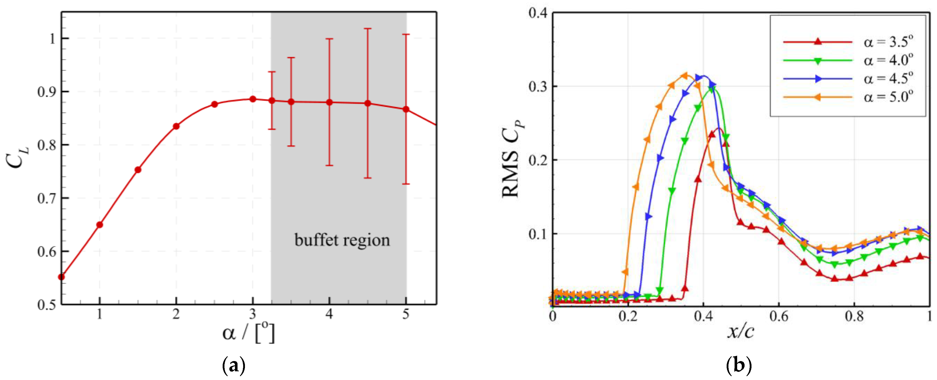
2.1. Baseline Airfoil

The OAT15A supercritical airfoil, which has been widely tested in wind tunnel experiments for studying the transonic buffet, was chosen as the baseline airfoil. In order to develop an extensive experimental database for validating the numerical methods, Jacquin et al. [3] performed the buffet experiment on the OAT15A airfoil section in the ONERA S3Ch transonic wind tunnel. The wind tunnel model is an OAT15A profile with a relative thickness of 12.3%, a chord length (c) of 230 mm, a span of 780 mm, and a blunt trailing edge of 0.5%c thickness. With the stagnation conditions of $P_{st}={10}^5\mathrm{Pa}$, $T_{st}=300\mathrm{K}$ and a Reynolds number of $R{e}_c=3\times {10}^6$, the flow Mach number varies in the range of 0.70 to 0.75, and the angle of attack between $2.5°$ and $3.91°$. The boundary layer transition is fixed at the 7%c on the upper and lower surfaces of the airfoil [3].

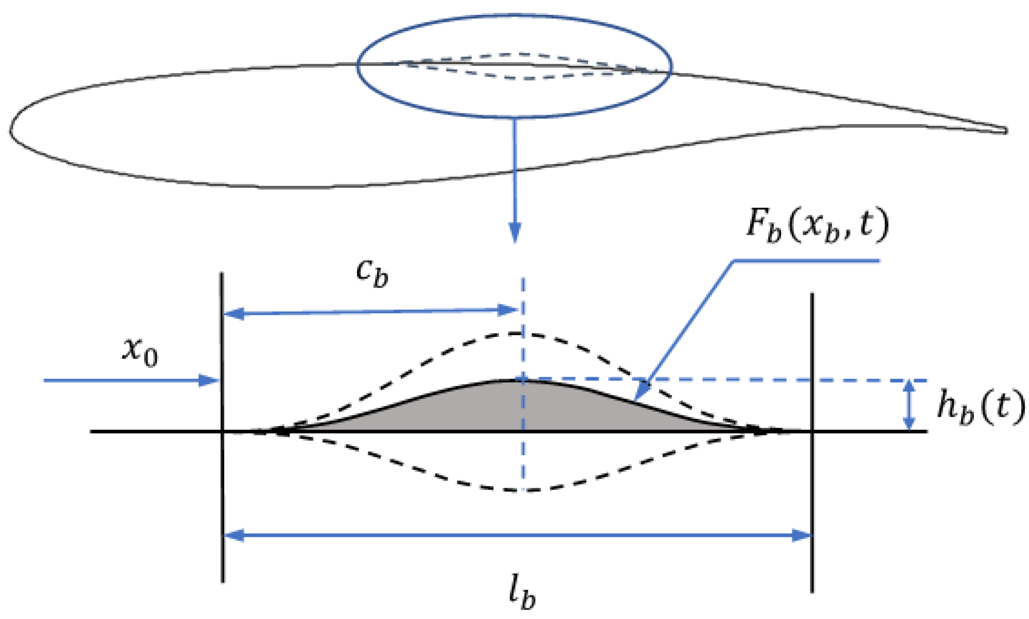
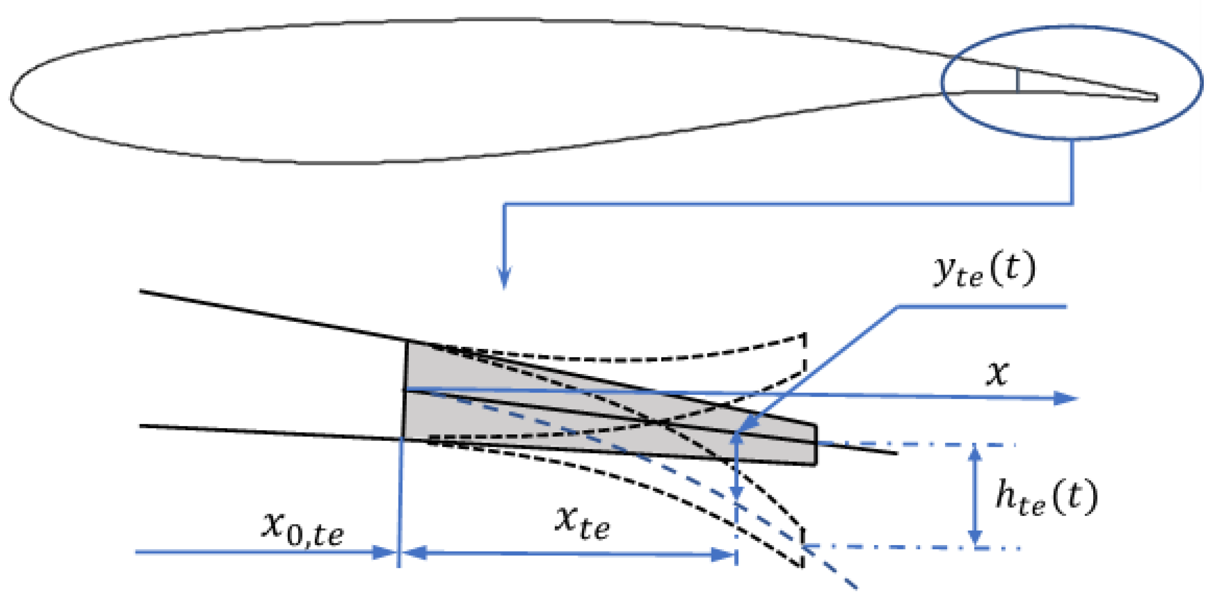
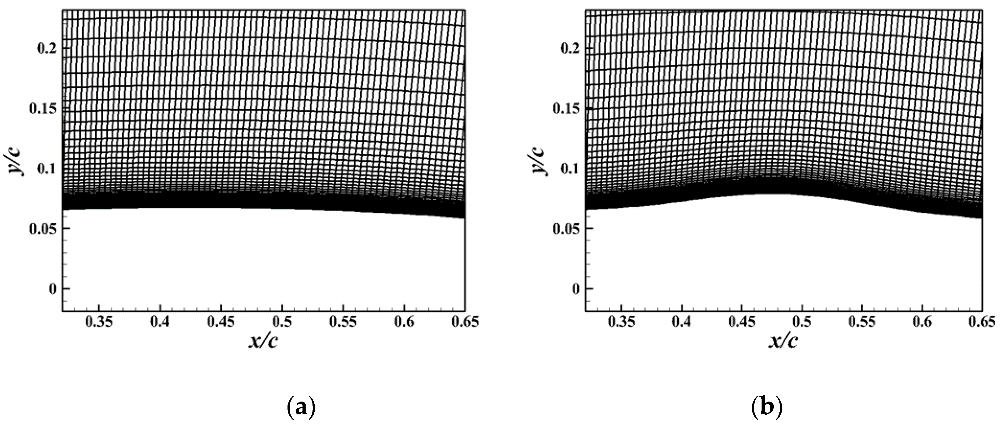
2.2. Definition of Active Control Devices

As shown in Figure 1, the active SCB is added on the upper surface of a given baseline airfoil, and the bump function represents the distance between the baseline airfoil and the bump surface. The bump length is denoted as $l_b$, and the bump crest position relative to the starting point is denoted as $c_b$. The coordinate of the bump crest can be obtained as:

$$x_c=(x_0+c_b)/c$$

(1)

where $x_0$ is the coordinate of the starting point of the bump. The local coordinate normalized by the bump length, $x_b$, satisfies

$$0\le x_b=\frac{x-x_0}{l_b}\le 1$$

(2)

The SCB shape function normalized by the bump height is defined by the Hicks-Henne function shown as:

$$\begin{array}{cc}H(x_b)={\sin }^4(\pi x_b{}^m),& m=\ln (0.5)/\ln (c_b/l_b)\end{array}$$

(3)

The resulting SCB function is therefore given by the following equation:

$$F_b(x_b,t)=h_b(t)\cdot H\left(x_b\right)$$

(4)

where $h_b\left(t\right)$ represents the transient bump height, which is a function of time t.

For comparison, the reference active trailing edge flap previously studied in [31] is presented as shown in Figure 2. The airfoil shape has been decomposed into the thickness distribution and the mean camber line. Only the mean camber line, denoted as $y_{te}$, will be changed in the TEF control. The mean camber line associated with the trailing edge flap is parameterized by a third-order polynomial. The starting location of the flap is denoted as $x_{0,te}$, and the flap length is given by $l_T=c-x_{0,te}$. The local coordinate of the flap normalized by the flap length is denoted as $x_{te}=(x-x_{0,te})/l_T$. The mean camber line associated with the trailing edge flap is defined as:

$$y_{te}=h_{te}(t)\cdot x_{te}{}^3$$

(5)

where $h_{te}\left(t\right)$ represents the transient displacement of the trailing edge.

Note that for an open-loop control such as the work of [28], $h_b\left(t\right)$ or $h_{te}\left(t\right)$ are specified by a user-defined function. For the closed-loop control, $h_b\left(t\right)$ or $h_{te}\left(t\right)$ are determined by the corresponding control law, which will be introduced in the next section.

2.3. Closed-Loop Control Law for Buffet Alleviation

Assuming that a real-time feedback signal, namely the lift coefficient here, can be obtained, the control devices defined in the previous section can be actively adjusted to suppress the lift oscillation by feedback control. Following the work of [20], the closed-loop control law is designed as follows:

$$h(t)=k(C_L(t-\Delta t)-C_{L0})$$

(6)

where $h\left(t\right)$ represents either the bump height, $h_b\left(t\right)$, or the displacement of the trailing edge, $h_{te}\left(t\right)$; $C_{L0}$ is the design lift coefficient; $\Delta t$ is the delay time, and $k$ is the gain to control the active device with the help of fluctuating lift coefficient $C_L\left(t\right)$. According to the control law, the control device will automatically adjust when the lift coefficient deviates from the design lift coefficient.

In unsteady simulations, the adjustment of the active control device can be regarded as surface deformation. The mesh is updated by a distance-based dynamic mesh algorithm [33]. As shown in Figure 3, the mesh near the active surface maintains a good quality and the far-field cells are largely unaffected.

3. Numerical Methods

3.1. Flow Solver

The compressible viscous flow was simulated by the open-source code CFL3D [34,35]. The governing equations were the unsteady Reynolds-averaged Navier-Stokes equations. An upwind Roe flux difference splitting algorithm with a third-order upwind MUSCL scheme was selected to resolve the inviscid fluxes to resolve the shock waves. The diffusive fluxes were treated using the second-order central differencing method. According to a recent study on the numerical methods for transonic buffet [10], the Spalart-Allmaras one-equation turbulence model was unable to produce shock unsteadiness on the OAT15A airfoil under the condition of $M_{\infty }=0.73$, $\alpha =3.5°$, and ${Re}_c=3\times {10}^6$, whereas the Stress-Omega Reynolds Stress Model (SORSM) amplified the pressure fluctuations. Menter’s k-ω SST model [36] with a reduced $a_1$ coefficient was found to be able to capture the shock unsteadiness properly. Based on our previous experiences [31], Menter’s k-ω SST turbulence model with the $a_1$ coefficient of 0.286 was used for the closure of the Reynolds-averaged Navier-Stokes equations. In addition, an implicit dual-time marching scheme was adopted and the physical (outer) time step size was chosen to be $2\times {10}^{-5}\mathrm{s}$, corresponding to about 750 time-steps per buffet cycle. The flow solution was assumed to be converged when the L2 norm of the residual reduced to ${10}^{-5}$ during the inner (pseudo-time) iterations.

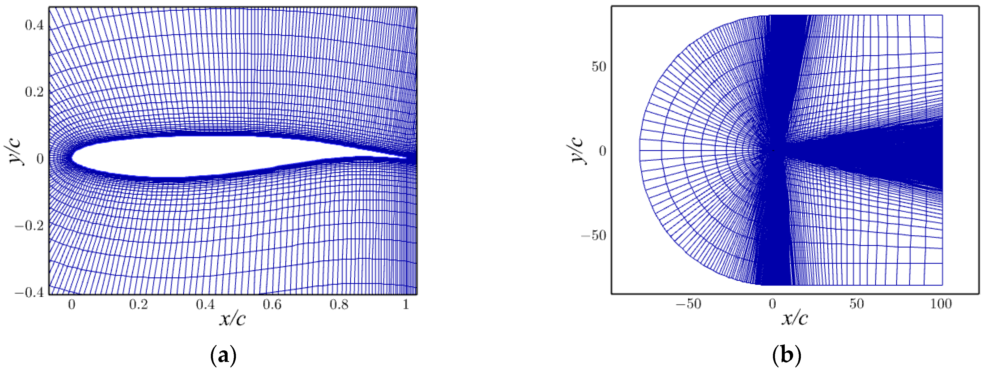
3.2. Grid Convergence Study

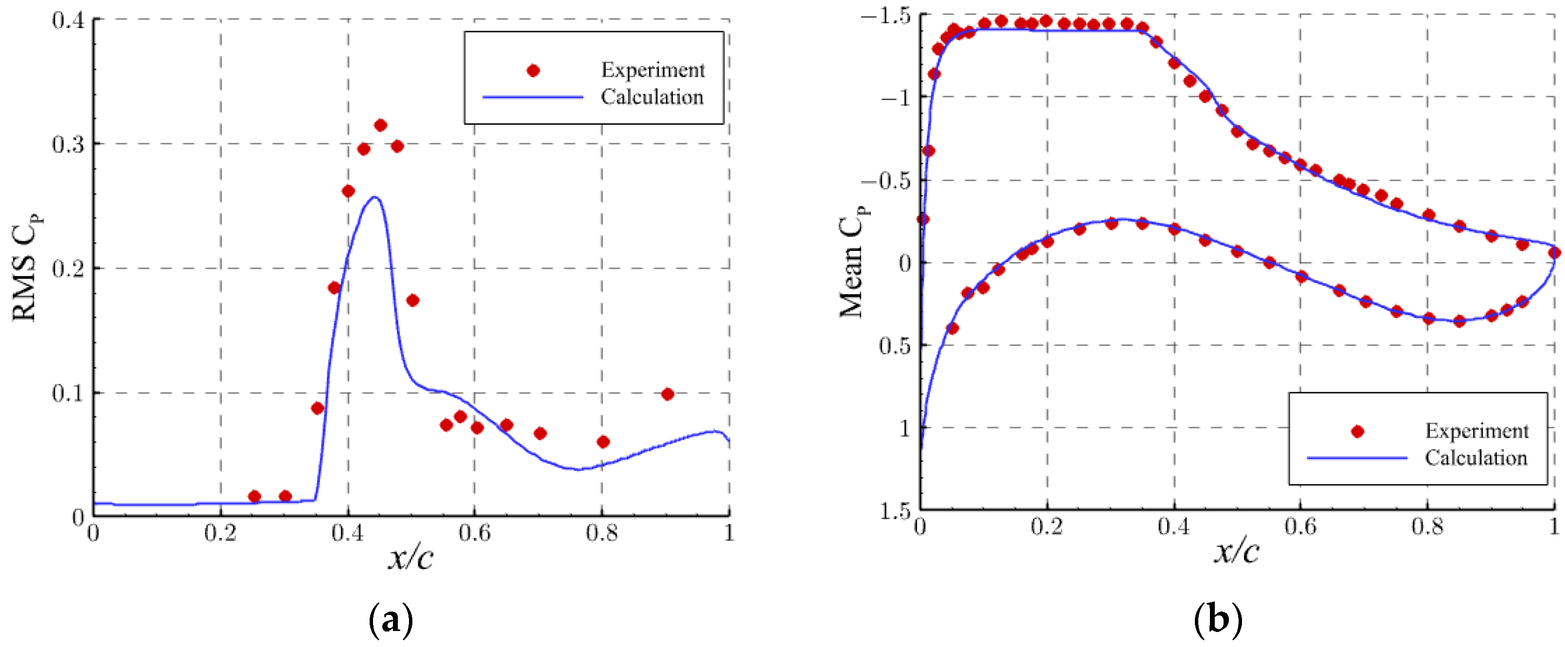
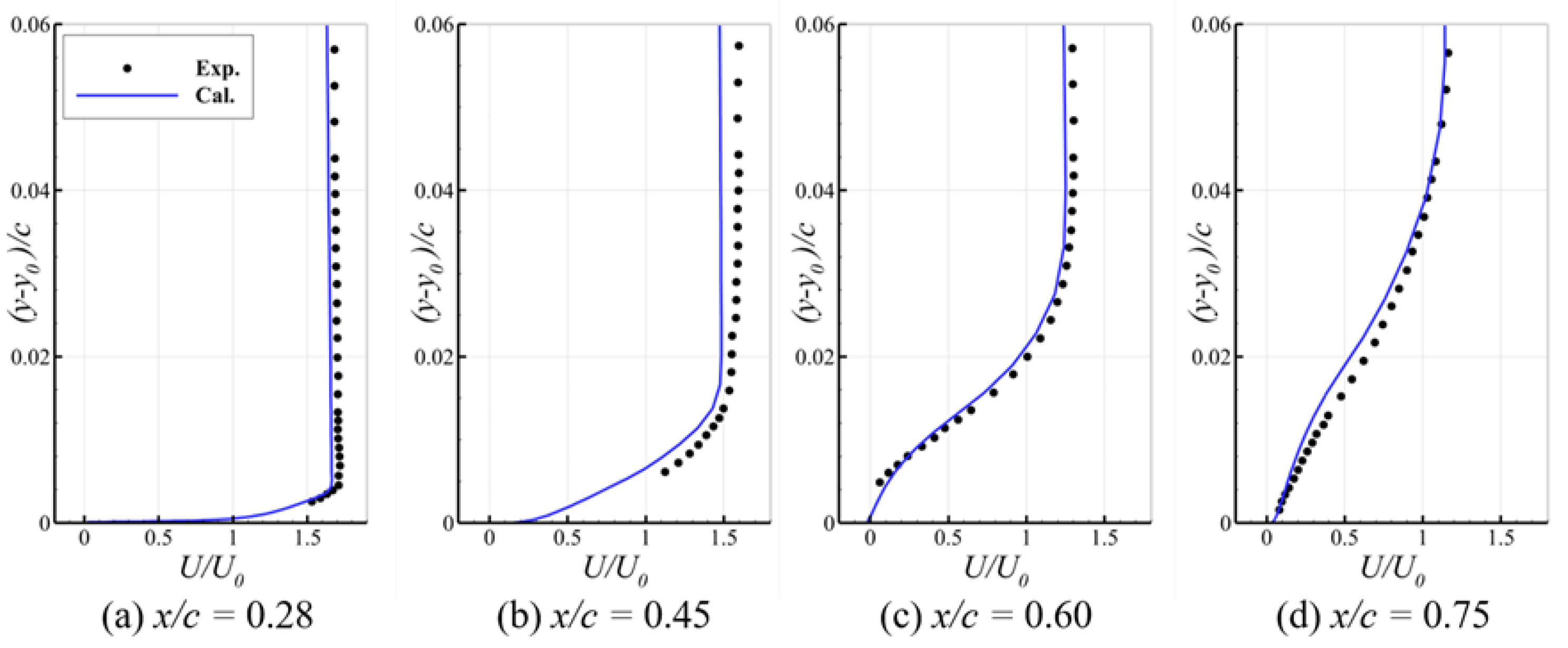
A C-type grid has been generated to carry out the simulations. The grid extends 80 chord lengths in the upstream and normal directions, and 100 chord lengths in the downstream direction illustrated in Figure 4. Three meshes of different grid densities named G1, G2, and G3 were created to assess the mesh independence, with the detailed parameters provided in

Table 1. The details of the computational grids.

Grid	Airfoil Nodes	First Layer	${\mathit{y}}_{\mathit{m}\mathit{a}\mathit{x}}^{+}$	Cell Count
G1	417	1.5 × 10−6	0.75	55,000
G2	517	1.2 × 10−6	0.70	83,000
G3	647	1.0 × 10−6	0.50	106,000

. In order to capture the shock wave accurately, the G2 grid near the trailing edge was refined, with the maximum cell size less than 0.5%c in the streamwise direction. A maximum wall $y^{+}<1$ was achieved at the boundary layer in the wall-normal direction of all grids, as required for the near-wall resolution of the turbulence model. The grid convergence was assessed under the condition of $M_{\infty }=0.73$, $\alpha =3.5°$, using the k-ω SST turbulence model and based on the computed buffet characteristics.

Table 2. The computed buffet characteristics using different levels of grid.

Grid	${\mathbf{\Delta }\mathit{C}}_{\mathit{L}}$	Mean ${\mathit{C}}_{\mathit{L}}$	${\mathit{f}}_{\mathit{s}\mathit{b}}$ (Hz)
G1	0.050	0.896	76
G2	0.166	0.881	75
G3	0.159	0.882	75
Experiment [3]	0.220	-	69

shows the results of the buffet characteristics, including the peak-to-peak lift difference, the mean lift coefficient, and the buffet frequency. The differences in the computed flow properties between the medium and finest grids are negligible. As a result, the mesh-independent solution is achieved with the G2 grid, and the G2 grid was employed for all subsequent simulations.

3.3. Validation

The comparison of the mean and RMS pressure coefficients on the upper surface of the airfoil is presented in Figure 5. Note that the RMS pressure coefficient is defined as ${\left(p-p_{ave}\right)}_{rms}/q_0$, where $p$, $p_{ave}$ and $q_0$ represent the static pressure, the mean static pressure, and the freestream dynamic pressure, respectively. The freestream flow conditions are $M_{\infty }=0.73$, $\alpha =3.5°$, and $R{e}_c=3\times {10}^6$. It can be observed that the predicted mean pressure coefficient shows good agreement with the experimental data. According to previous studies [37,38], the peak pressure fluctuation and the pressure fluctuation are sensitive to the turbulence model and the flow transition location. Although the peak pressure fluctuation and the pressure fluctuation near the trailing edge are slightly lower than the experimental data, the shock movement is well captured by the numerical simulation. The mean velocity profiles at different stations on the upper surface of the airfoil are shown in Figure 6. It can be seen that the calculated results match well with the experimental data, consistent with the results of [5,7,10].

4. Results and Discussions

4.1. The Design of the Active SCB

In previous studies, it was found that the bump crest location was the key parameter for both wave drag reduction and buffet suppression. Tian et al. [27] showed that passive SCBs positioned between 10 and 18% aft of the mean shock location were capable of suppressing shock oscillations in a buffeting flow field. Furthermore, Geoghegan et al. [28,29,30] showed that for the OAT15A airfoil with oscillating SCBs, buffet suppression existed for a much wider range of positions including SCBs positioned aft and in front of the mean shock location.

Figure 7 shows the range of the shock movement on the upper surface of the OAT15A airfoil. The freestream flow conditions are $M_{\infty }=0.73$, $\alpha =3.5°$, and $R{e}_c=3\times {10}^6$. It can be estimated that the upper and lower limits of shock location are 0.44c and 0.54c, respectively, resulting in a mean shock location of 0.49c. Therefore, in this study, the bump crest is fixed at the mean shock location, i.e., x_c = 0.49c. In addition, the active SCB is designed to be symmetrical and has a length of 0.3c, according to our previous study [31].

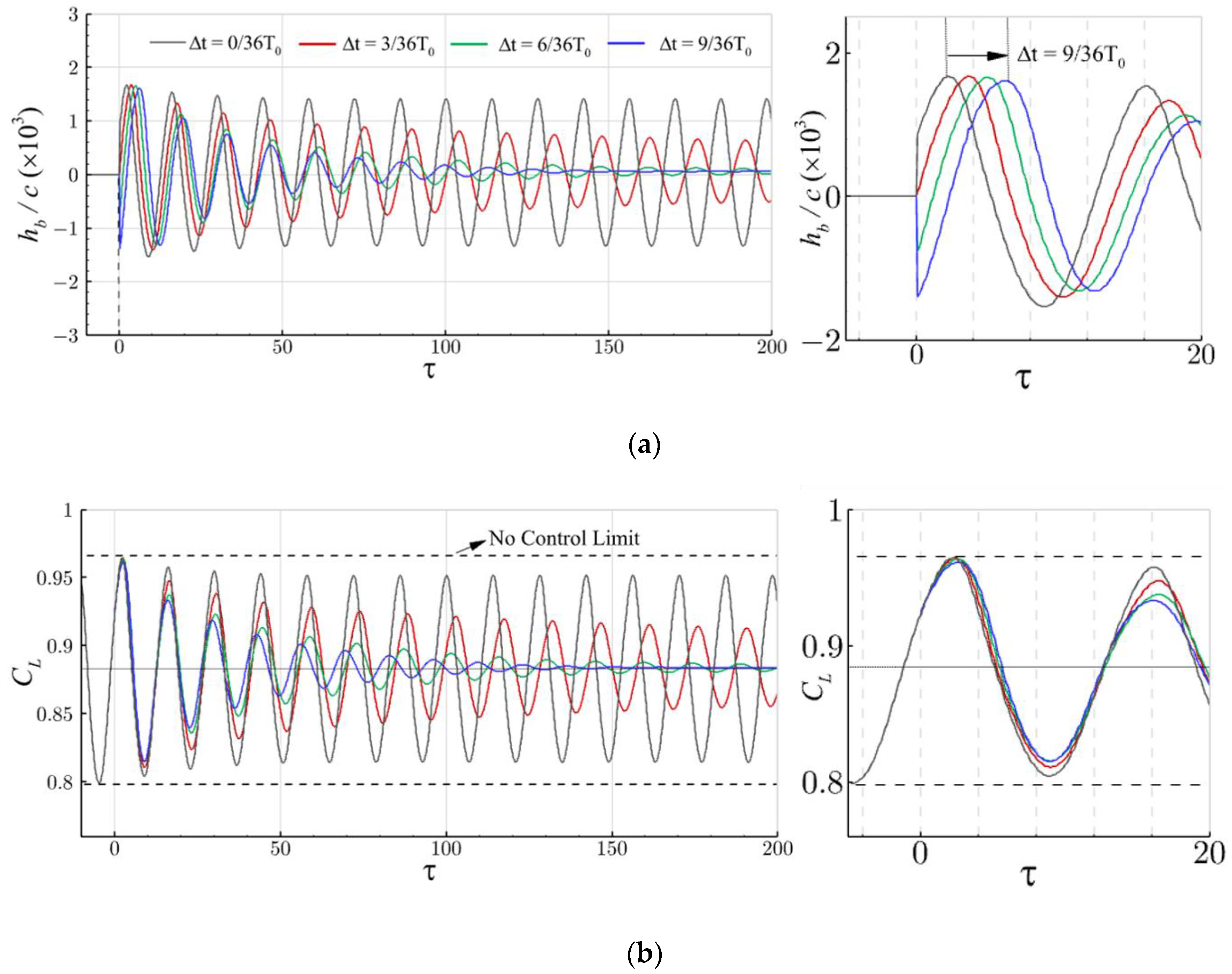
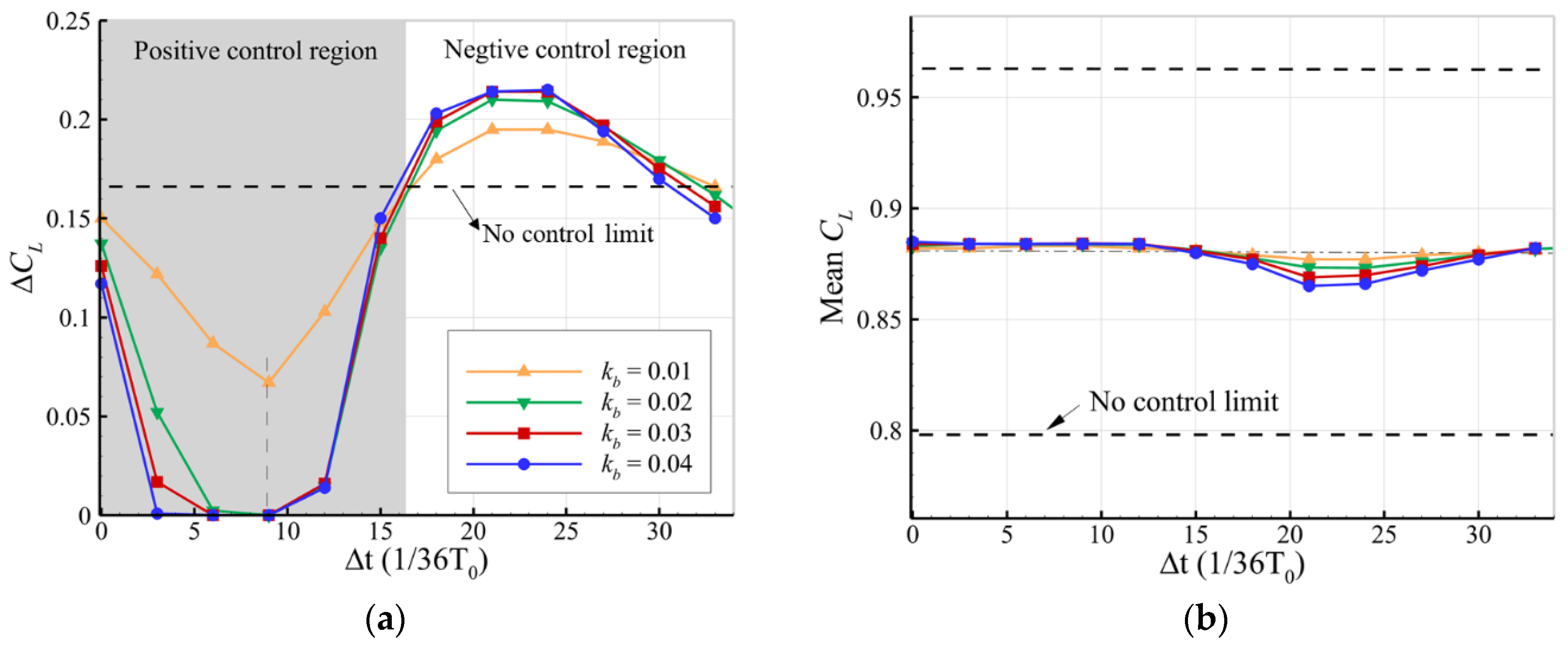
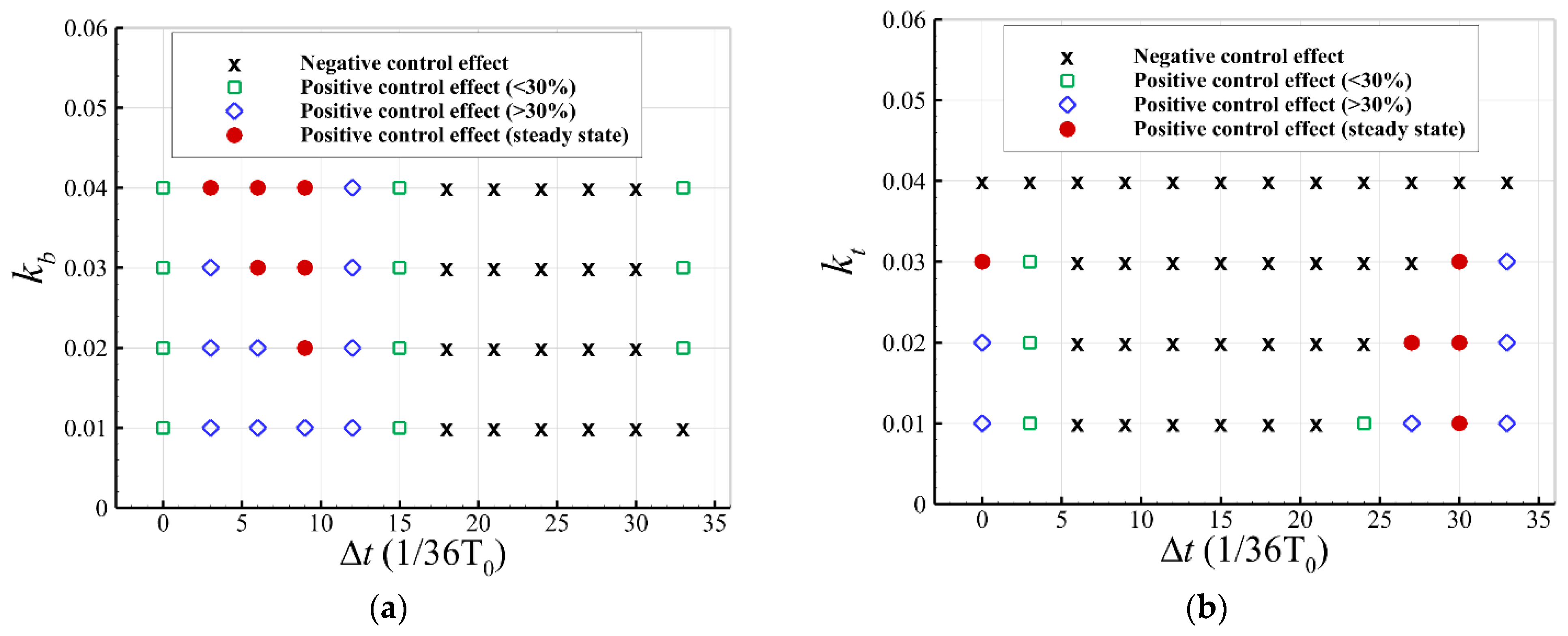
4.2. The Effects of Parameters of the Control Law on Buffet Alleviation

According to the closed-loop control law shown in Equation (6), there are two parameters, namely the gain, $k_b$, and the delay time, $\Delta t$. The effect of the gain will be first studied. The freestream flow conditions are chosen as $M_{\infty }=0.73$, $\alpha =3.5°$, and $R{e}_c=3\times {10}^6$, corresponding to a typical buffet case for the OAT15A airfoil. The delay time, $\Delta t$, was set to 0, and the design lift coefficient, $C_{L0}$, was set to 0.881, which is equal to the mean lift coefficient of the baseline airfoil.

Figure 8 shows the time history of the responses by the active SCB with different gains. Note that the non-dimensional time was defined as $\tau =t·U/c$, where $t$ and $U$ represent the flow time and the reference velocity, respectively. The active SCB is deployed at $\tau =0$ and runs until the steady-state flow is detected or the solution locks into a new buffet state. It can be seen that the active SCB can slightly suppress the amplitude of lift fluctuation. As shown in Figure 8b, with the increase of the gain, the amplitude of lift fluctuation decreases. However, as $k_b$ increases to 0.05, only 30% of the lift amplitude has been reduced. Therefore, it can be concluded that the gain has a relatively minor effect on buffet suppression, and the effect of the delay time should be taken into consideration as well.

Based on the above studies, we fixed the gain as $0.02$ and investigated the effect of the delay time on buffet suppression. Here the delay time, $\Delta t$, is described by the buffet period, $T_0$, of the baseline airfoil. For example, $\Delta t=9/36T_0$ means that the phase of the height fluctuation has a lag of 90° relative to that of the lift fluctuation. Figure 9 shows the time history of the responses under the control with the delay time ranging from 0 to $9/36T_0$. When the delay time is set to $3/36T_0$, the lift amplitude decreases by approximately 70% of that of the baseline airfoil. When $\Delta t$ becomes $6/36T_0$, the lift fluctuation is almost suppressed to a steady state within about 200 non-dimensional time. When $\Delta t$ becomes $9/36T_0$, a stable flow is quickly established.

The parameter space for closed-loop control was explored by studying various combinations of the gain and the delay time. Figure 10 shows the amplitude of lift fluctuation and the mean lift coefficient by using various parameters of the control law. It is clear that the active SCB is effective for buffet alleviation by using the delay time ranging from 0 to $15/36T_0$. Moreover, it can be found that the optimal delay time is equal to $9/36T_0$, independent of the gain. In addition, it can be observed that the mean lift coefficient slightly increases under an effective closed-loop control.

Figure 11 shows the time history of the responses by using the optimal delay time ($\Delta t=9/36T_0$) and different gains. To analyze the performances of the control system for a quadrotor UAV, several performance indicators were used by Liu et al. [39,40]. In the current study, following the work of [30], the settling time, denoted as $\Delta {\tau }_{s.t.}$, is adopted to quantify the response speed of the control system. It is defined as the non-dimensional time when the amplitude of lift fluctuation decreases by 90% of that of the baseline airfoil. By adopting $k_b=0.02$, the settling time is $104$ and the maximum bump height is about 0.0016c. When the gain increases to 0.04, the settling time decreases to $23$ and the maximum bump height increases to 0.003c. This means that the control system has a shorter response time by using a larger gain, at the cost of a higher bump height.

Figure 12 shows the relation between the bump movement and the shock movement for the case of $k_b=0.02$ and $\Delta t=9/36T_0$. Note that the dash lines in the figure are the limits of shock movement. It can be observed that as the shock moves from the lower limit (point a) to the upper limit (point c), a bump with positive camber is needed to suppress the shock movement. Inversely, as the shock moves from the upper limit (point c) to the lower limit (point e), a bump with negative camber is needed.

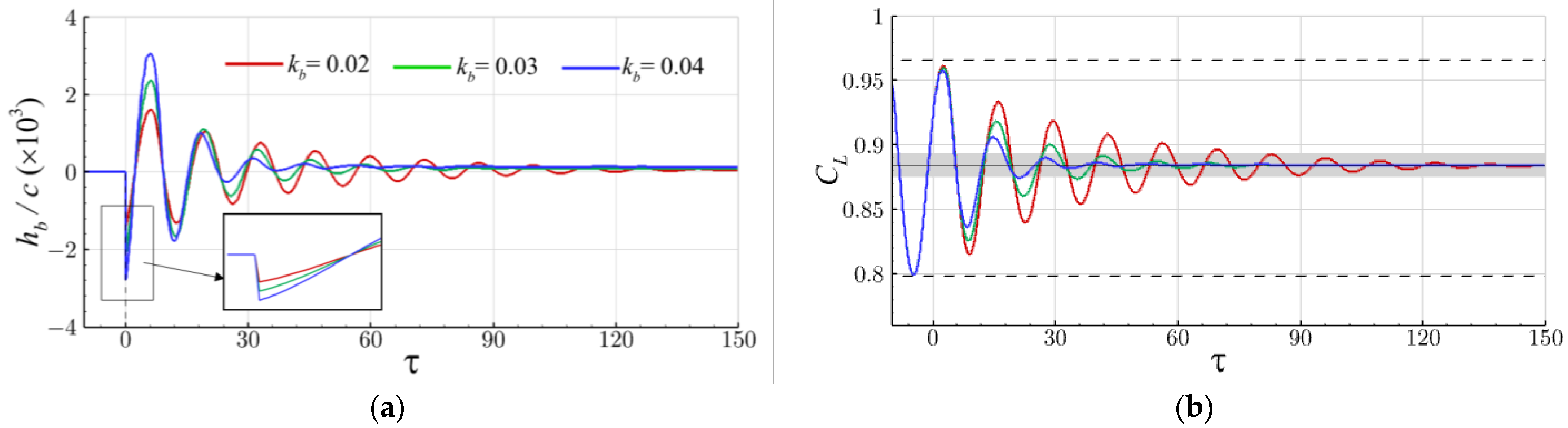
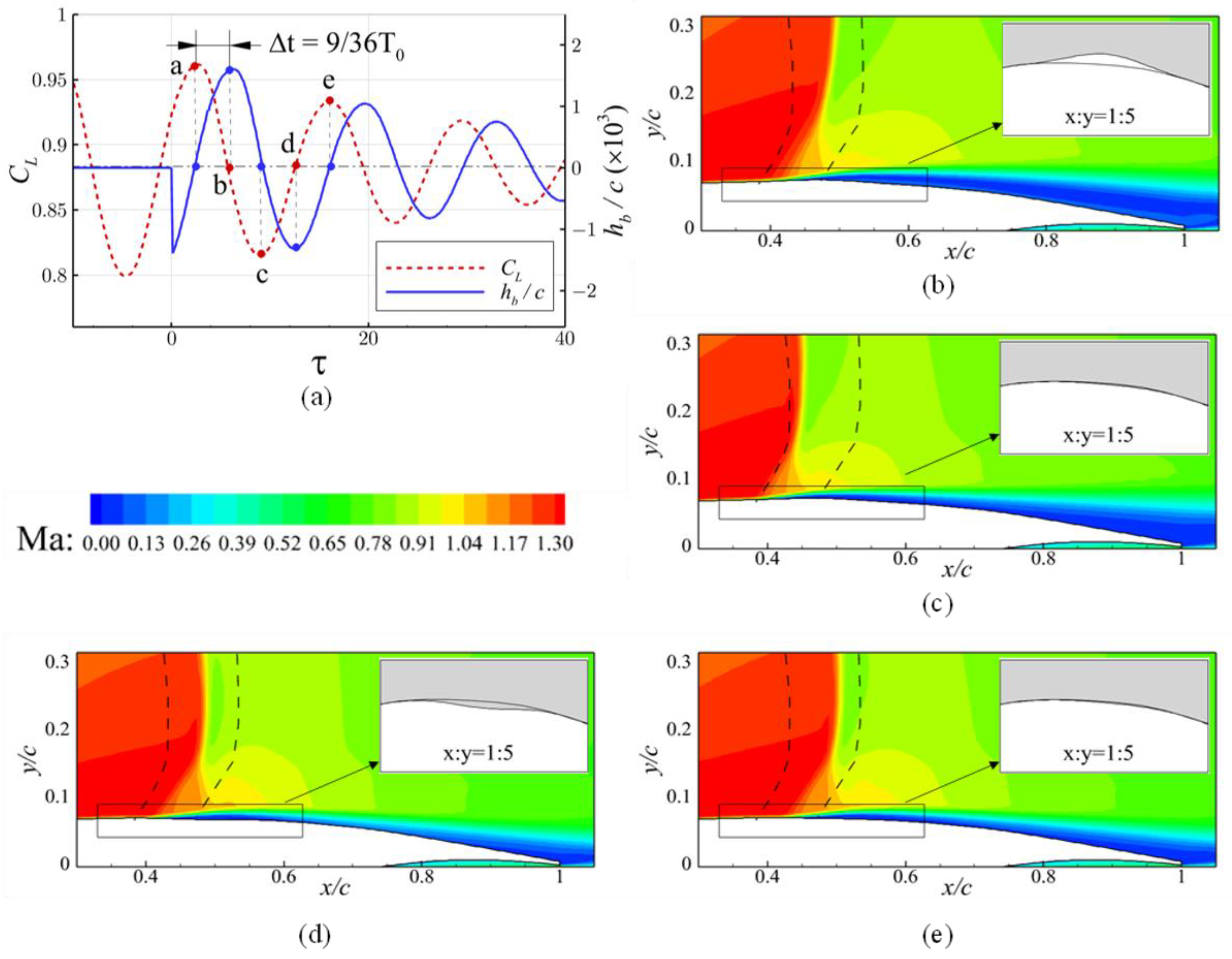
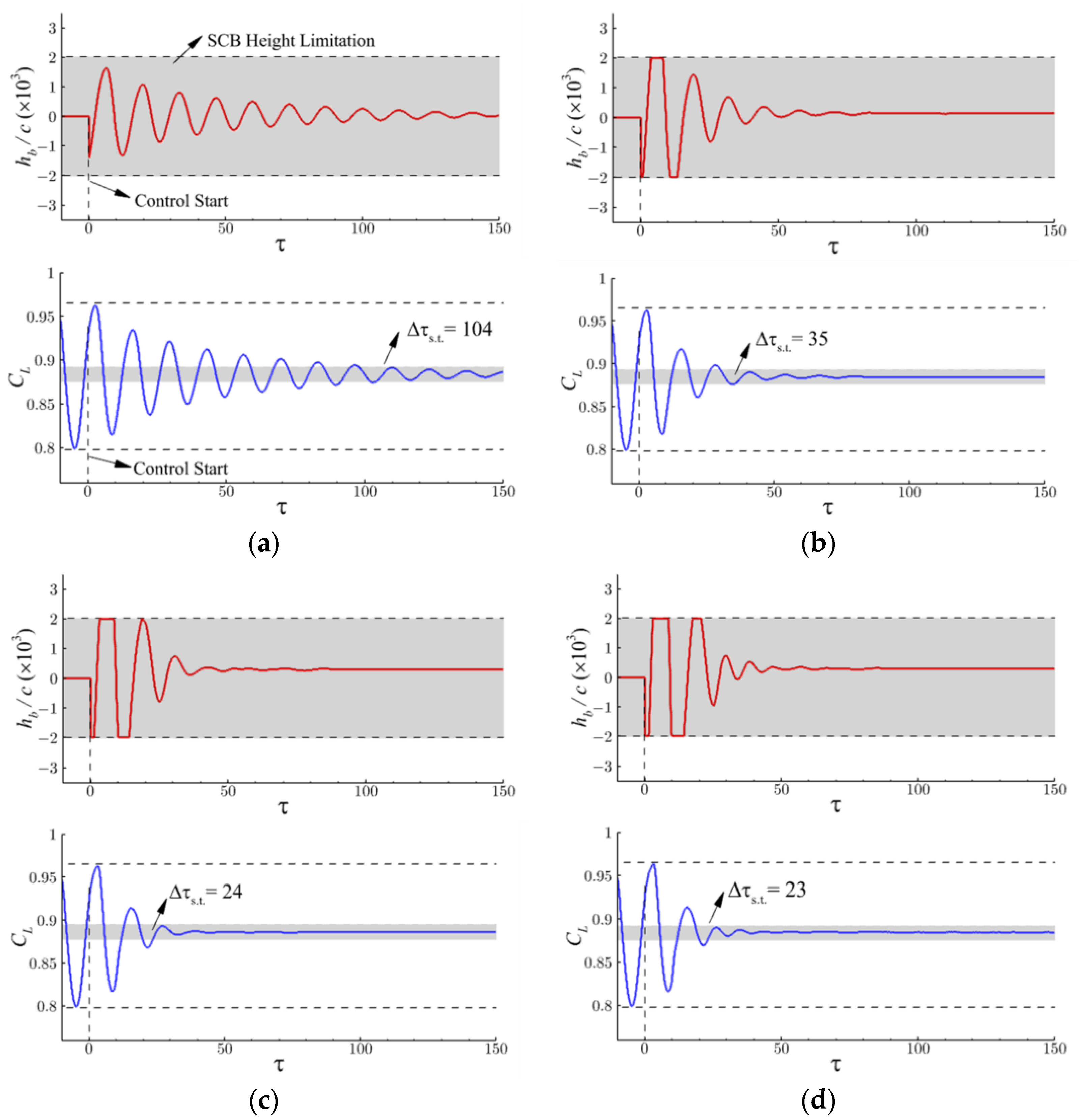
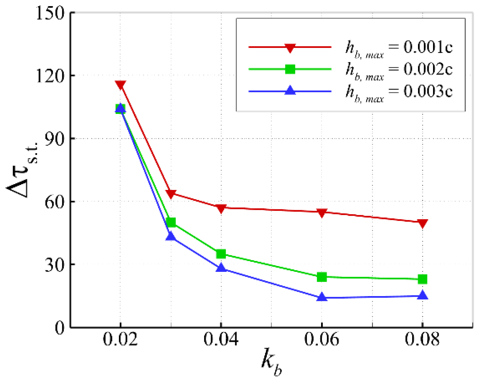
4.3. Buffet Control Constrained by Maximum Bump Height

The above study shows that the active SCB with a larger gain has better performance in suppressing the buffet. However, the resulting high bump will bring new challenges for practical applications due to the deformation achievable on the wings. In this section, we consider imposing a constraint on the maximum height of the active SCB. The closed-loop control law is redesigned as follows:

$$h_b=\left\{\begin{array}{l}{k}_b\left(C_L\left(t-\Delta t\right)-C_{L0}\right),\left|h_b\right|<h_{b,max}\\ h_{b,max},\left|h_b\right|\ge h_{b,max}\end{array}\right.$$

(7)

where $h_{b,max}$ is the maximum bump height.

Figure 13 shows the response of the lift coefficient by using different gains. The maximum bump height of the active SCB is set to 0.002c. In the case of $k_b=0.02$, as shown in Figure 13a, the actual bump height is no more than the maximum height. As a result, the responses are identical to that of the previous control law without a height constraint. The settling time is 104. In the case of $k_b=0.04$, as shown in Figure 13b, the bump height reaches the height limit. The settling time is $35$, showing an improvement in response speed. When the gain increases to $0.06$, as shown in Figure 13c, the settling time reduces to 24. As the gain continues to increase to 0.08, as shown in Figure 13d, very little improvement can be observed with regard to the settling time. It can be concluded that by imposing a height constraint on the closed-loop system, its response speed can be significantly increased by using a large gain.

Figure 14 shows the change in the settling time with the gain by imposing various height constraints. It is clear that the settling time can be effectively reduced by increasing the gain. In addition, loosening the height constraint can further decrease the settling time. However, as the gain exceeds 0.06, no apparent improvement can be observed in the response speed.

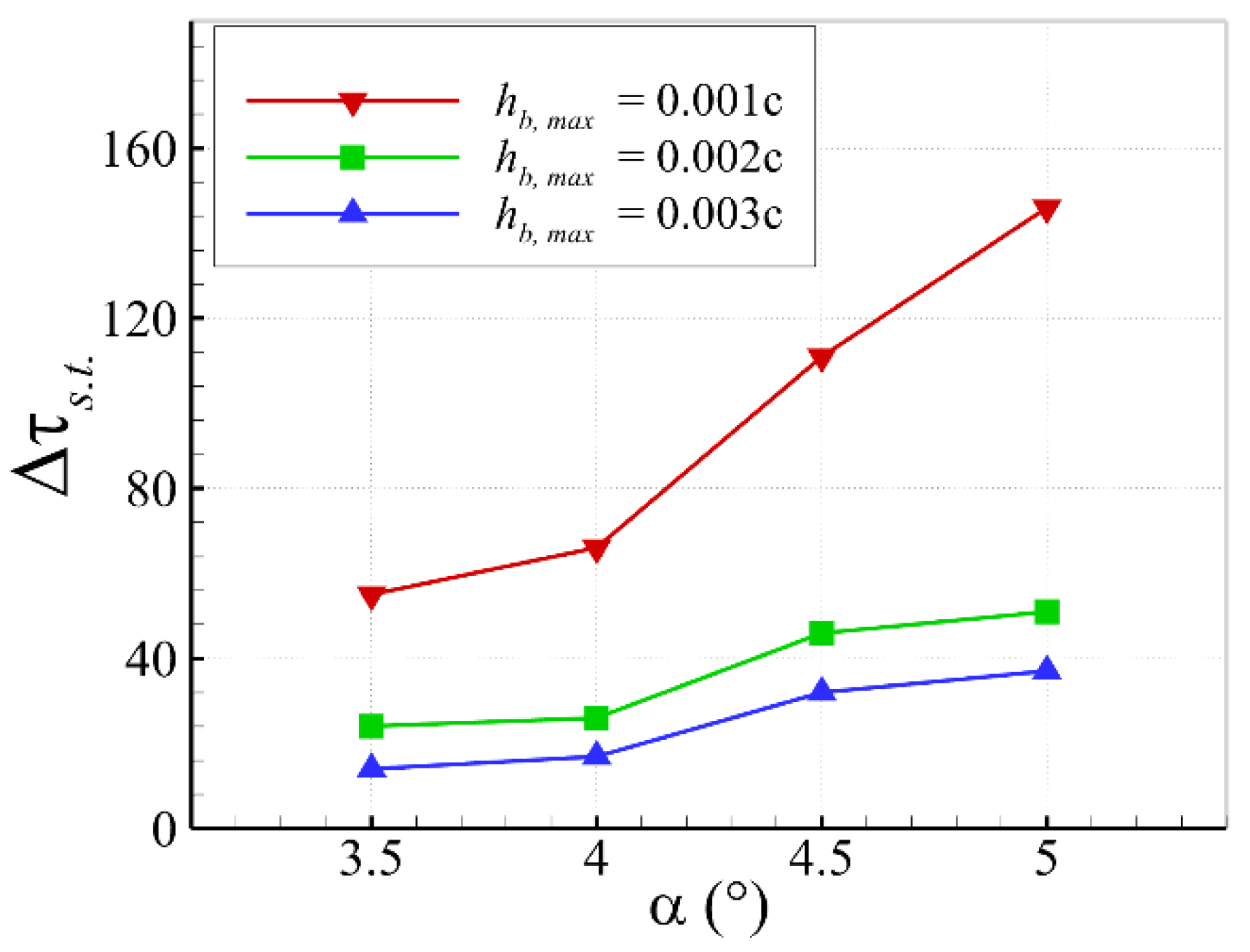
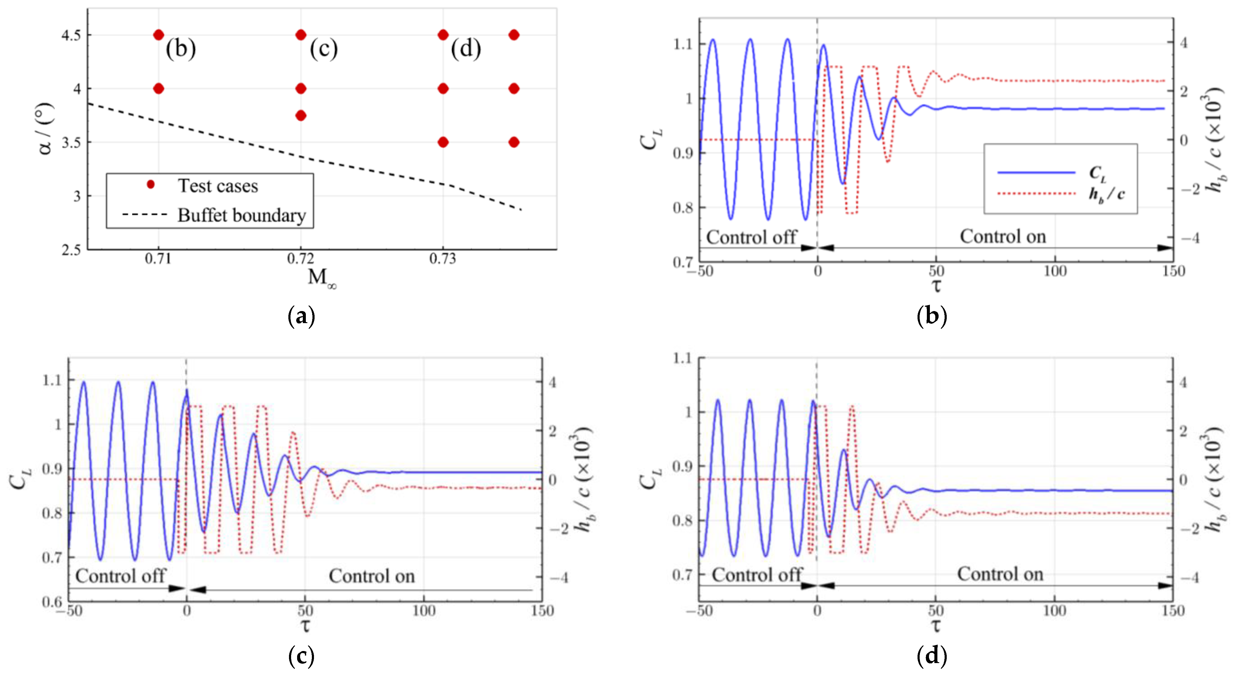
4.4. Buffet Control over a Range of Flow Conditions

This section will investigate the robustness of the closed-loop control system under various flow conditions. First, the angle of attack is changed, while the other flow conditions are fixed as $M_{\mathrm{\infty }}=0.73$ and $R{e}_c=3\times {10}^6$. Figure 15 shows the lift coefficients and RMS pressure coefficients for the baseline airfoil at an angle of attack ranging from 3.5° to 5.0°. It can be found that with the increase in the angle of attack, the amplitude of lift fluctuation gradually increases and the range of shock motion increases as well. In addition, the mean shock location also changes as the angle of attack varies.

The same active SCB with a gain of 0.06 and a delay time of $9/36T_0$ has been adopted for all cases ranging from 3.5° to 5.0° at $M_{\mathrm{\infty }}=0.73$. Figure 16 shows the variation of the settling time with the angle of attack. It can be seen that as the angle of attack increases, the settling time gradually increases, meaning that the response speed decreases. However, this problem can be relieved by increasing the bump height. As the maximum bump height increases to 0.002c, the settling time is relatively insensitive to the angle of attack. Overall, it can be concluded that the closed-loop control system has good robustness over a range of angles of attack by using an optimal combination of parameters of the control law.

Then, the active SCB with a gain of 0.06, a delay time of $9/36T_0$, and a maximum height of $0.003c$ has been adopted to test the effectiveness of buffet control over a range of flow conditions. As shown in Figure 17a, the red dots indicate the chosen flow conditions. At these flow conditions, it was found that the fluctuating loads could be completely suppressed with the closed-loop control. Figure 17b–d shows the responses of airfoil lift and bump height at the angle of attack of $4.5°$. It can be seen that the control device can achieve buffet suppression in a short settling time. Therefore, it can be concluded that the closed-loop control has the ability to control the buffet over a wide range of flow conditions.

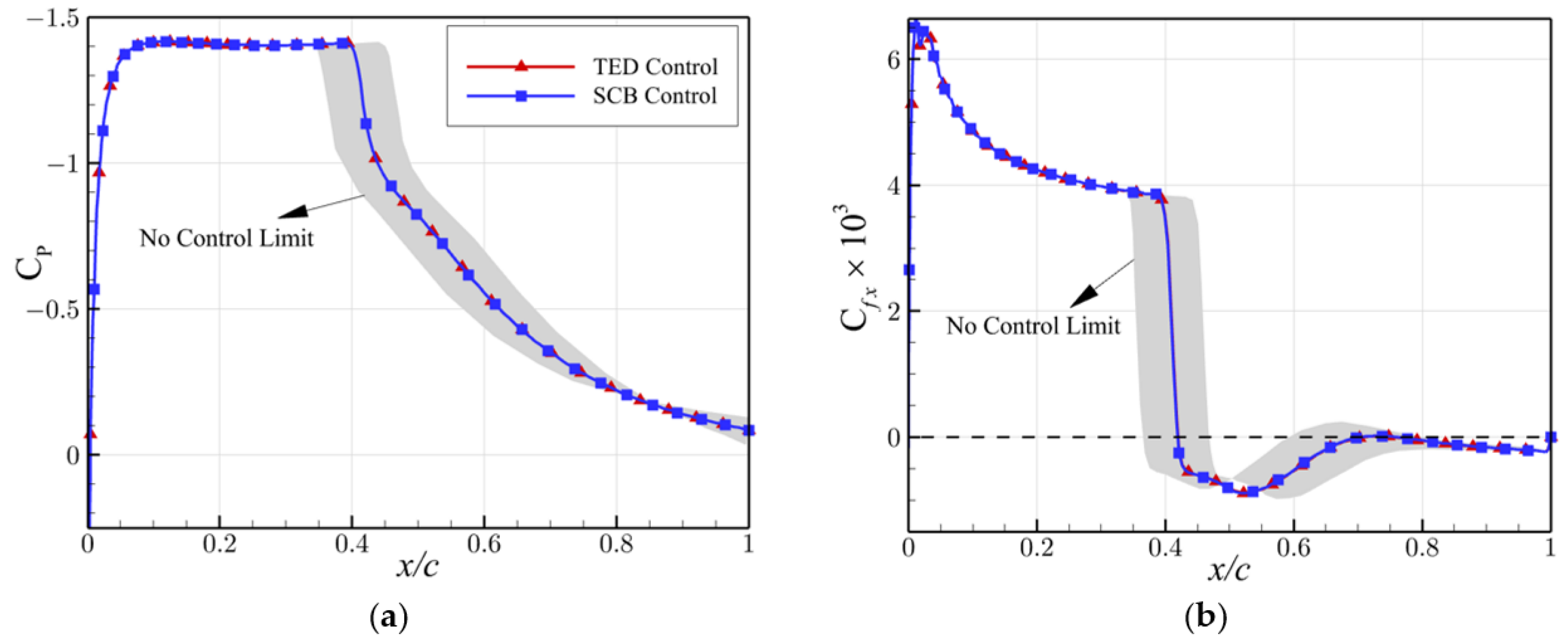
4.5. Comparison of Active Closed-Loop Buffet Control Using SCB and TEF

This section will compare the proposed buffet control method with the reference active TEF. The active TEF has a length of 0.1c, the same as in the study of [35]. The freestream flow conditions are chosen as $M_{\mathrm{\infty }}=0.73$, $\alpha =3.5°$, and $R{e}_c=3\times {10}^6$. Figure 18 shows the comparison of parameter spaces of two control methods. In the figure, the symbol “$\times$” indicates a negative control, i.e., increasing the amplitude of lift fluctuation. The symbols “□” and “◊” indicate that the control is able to reduce the lift amplitude. The symbol “□” represents the case that the reduction of the lift amplitude is less than 30% of that of the baseline airfoil, while the symbol “◊” represents the case that the reduction of the lift amplitude is more than 30% of that of the baseline airfoil. The symbol “○” indicates a fully positive control. It is clear that the effective region of buffet suppression using the active SCB is larger than that of using the active TEF. Therefore, the active SCB is less sensitive to the parameters of the control law, which is beneficial for the control system to work in a complex environment.

The fully controlled cases are further examined. Figure 19 shows the comparison of the steady state $C_p$ and $C_{fx}$ under the control methods. It can be seen that the two control methods produce almost identical results. This is also confirmed by the aerodynamic coefficients, as shown in

Table 3. Comparison of performances between the two control methods with a gain of 0.02.

Control Type	${\mathit{C}}_{\mathit{L}}$	${\mathit{C}}_{\mathit{D}}$	$\mathbf{\Delta }{\mathbf{\tau }}_{\mathit{s}.\mathit{t}.}$
Baseline (Mean)	0.881	0.0398	-
Active trailing edge flap	0.881	0.0390	93
Active bump	0.881	0.0389	37

. However, the settling time of buffet suppression using the active SCB is only 40% of that of using the active trailing edge flap. Overall, the proposed active SCB significantly outperforms the active TEF in terms of both robustness and response speed.

5. Conclusions

A closed-loop buffet control using an active shock control bump has been proposed and investigated. A closed-loop control law has been designed by using the lift coefficient as the feedback signal and using the bump height as the control variable. The location of the active SCB has been located according to the mean shock location of the baseline airfoil. The numerical tests based on the URANS simulations show that the proposed control method can effectively suppress the transonic buffet on a supercritical airfoil. The effects of parameters of the control law, including the delay time and the gain, on buffet suppression have been studied. It was found that when the phase of height fluctuation has a lag of $90°$ relative to the phase of lift fluctuation, the closed-loop system shows the best performance in alleviating the buffet. Considering the potential practical constraint on SCB height, the closed-loop control law was redesigned by imposing a height constraint, which also showed a good performance. Furthermore, the proposed SCB closed-loop buffet control system shows good robustness over a range of angles of attack. In comparison with the reference active TEF, the study shows that the active SCB is less sensitive to the parameters of the control law and has a shorter response time. In terms of both robustness and response time, the active SCB significantly outperforms the reference active TEF. The future works include applying the active SCB on three-dimensional wings and adopting more intelligent control algorithms, such as neural networks and sliding mode control.

References

1. Li, R.; Deng, K.; Zhang, Y.; Chen, H. Pressure Distribution Guided Supercritical Wing Optimization. Chin. J. Aeronaut. 2018, 31, 1842–1854. [Google Scholar] [CrossRef]
2. Lee, B.H.K. Self-Sustained Shock Oscillations on Airfoils at Transonic Speeds. Prog. Aerosp. Sci. 2001, 37, 147–196. [Google Scholar] [CrossRef]
3. Jacquin, L.; Molton, P.; Deck, S.; Maury, B.; Soulevant, D. Experimental Study of Shock Oscillation over a Transonic Supercritical Profile. AIAA J. 2009, 47, 1985–1994. [Google Scholar] [CrossRef]
4. Deck, S. Numerical Simulation of Transonic Buffet over a Supercritical Airfoil. AIAA J. 2005, 43, 1556–1566. [Google Scholar] [CrossRef] [Green Version]
5. Grossi, F.; Braza, M.; Hoarau, Y. Prediction of Transonic Buffet by Delayed Detached-Eddy Simulation. AIAA J. 2014, 52, 2300–2312. [Google Scholar] [CrossRef] [Green Version]
6. Zhang, Y.; Yang, P.; Li, R.; Chen, H. Unsteady Simulation of Transonic Buffet of a Supercritical Airfoil with Shock Control Bump. Aerospace 2021, 8, 203. [Google Scholar] [CrossRef]
7. Huang, J.; Xiao, Z.; Liu, J.; Fu, S. Simulation of Shock Wave Buffet and Its Suppression on an OAT15A Supercritical Airfoil by IDDES. Sci. China Phys. Mech. Astron. 2012, 55, 260–271. [Google Scholar] [CrossRef]
8. Levy, L.L., Jr. Experimental and Computational Steady and Unsteady Transonic Flows about a Thick Airfoil. AIAA J. 1978, 16, 564–572. [Google Scholar] [CrossRef]
9. Iovnovich, M.; Raveh, D.E. Reynolds-Averaged Navier-Stokes Study of the Shock-Buffet Instability Mechanism. AIAA J. 2012, 50, 880–890. [Google Scholar] [CrossRef]
10. Giannelis, N.F.; Levinski, O.; Vio, G.A. Influence of Mach Number and Angle of Attack on the Two-Dimensional Transonic Buffet Phenomenon. Aerosp. Sci. Technol. 2018, 78, 89–101. [Google Scholar] [CrossRef]
11. Giannelis, N.F.; Levinski, O.; Vio, G.A. Origins of a Typical Shock Buffet Motions on a Supercritical Aerofoil. Aerosp. Sci. Technol. 2020, 107, 106304. [Google Scholar] [CrossRef]
12. Smith, A.N.; Babinsky, H.; Fulker, J.L.; Ashill, P.R. Normal Shock Wave-Turbulent Boundary-Layer Interactions in the Presence of Streamwise Slots and Grooves. Aeronaut. J. 2002, 106, 493–500. [Google Scholar] [CrossRef]
13. Holden, H.A.; Babinsky, H. Separated Shock-Boundary-Layer Interaction Control Using Streamwise Slots. J. Aircr. 2005, 42, 166–171. [Google Scholar] [CrossRef]
14. Eastwood, J.P.; Jarrett, J.P. Toward Designing with Three-Dimensional Bumps for Lift/Drag Improvement and Buffet Alleviation. AIAA J. 2012, 50, 2882–2898. [Google Scholar] [CrossRef]
15. Holden, H.; Babinsky, H. Effect of Microvortex Generators on Seperated Normal Shock/Boundary Layer Interactions. J. Aircr. 2007, 44, 170–174. [Google Scholar] [CrossRef]
16. Rybalko, M.; Babinsky, H.; Loth, E. Vortex Generators for a Normal Shock/Boundary Layer Interaction with a Downstream Diffuser. J. Propuls. Power 2012, 28, 71–82. [Google Scholar] [CrossRef]
17. Caruana, D.; Mignosi, A.; Robitaillié, C.; Corrège, M. Separated Flow and Buffeting Control. Flow Turbul. Combust. 2003, 71, 221–245. [Google Scholar] [CrossRef]
18. Caruana, D.; Mignosi, A.; Corrège, M.; Le Pourhiet, A.; Rodde, A.M. Buffet and Buffeting Control in Transonic Flow. Aerosp. Sci. Technol. 2005, 9, 605–616. [Google Scholar] [CrossRef]
19. Dandois, J.; Lepage, A.; Dor, J.-B.; Molton, P.; Ternoy, F.; Geeraert, A.; Brunet, V.; Coustols, É. Open and Closed-Loop Control of Transonic Buffet on 3D Turbulent Wings Using Fluidic Devices. Comptes Rendus Mec. 2014, 342, 425–436. [Google Scholar] [CrossRef]
20. Gao, C.; Zhang, W.; Ye, Z. Numerical Study on Closed-Loop Control of Transonic Buffet Suppression by Trailing Edge Flap. Comput. Fluids 2016, 132, 32–45. [Google Scholar] [CrossRef]
21. Ren, K.; Chen, Y.; Gao, C.; Zhang, W. Adaptive Control of Transonic Buffet Flows over an Airfoil. Phys. Fluids 2020, 32, 096106. [Google Scholar] [CrossRef]
22. Birkemeyer, J.; Rosemann, H.; Stanewsky, E. Shock Control on a Swept Wing. Aerosp. Sci. Technol. 2000, 4, 147–156. [Google Scholar] [CrossRef]
23. Qin, N.; Zhu, Y.; Shaw, S.T. Numerical Study of Active Shock Control for Transonic Aerodynamics. Int. J. Numer. Methods Heat Fluid Flow 2004, 14, 444–466. [Google Scholar] [CrossRef]
24. Qin, N.; Wong, W.; Le Moigne, A. Three-Dimensional Contour Bumps for Transonic Wing Drag Reduction. Proc. Inst. Mech. Eng. Part G J. Aerosp. Eng. 2008, 222, 619–629. [Google Scholar] [CrossRef]
25. Mayer, R.; Lutz, T.; Krämer, E. Numerical Study on the Ability of Shock Control Bumps for Buffet Control. AIAA J. 2018, 56, 1978–1987. [Google Scholar] [CrossRef]
26. Mayer, R.; Lutz, T.; Krämer, E.; Dandois, J. Control of Transonic Buffet by Shock Control Bumps on Wing-Body Configuration. J. Aircr. 2019, 56, 556–568. [Google Scholar] [CrossRef]
27. Tian, Y.; Gao, S.; Liu, P.; Wang, J. Transonic Buffet Control Research with Two Types of Shock Control Bump Based on RAE2822 Airfoil. Chin. J. Aeronaut. 2017, 30, 1681–1696. [Google Scholar] [CrossRef]
28. Geoghegan, J.A.; Giannelis, N.F.; Vio, G.A. A Numerical Study on Transonic Shock Buffet Alleviation through Oscillating Shock Control Bumps. In Proceedings of the 2018 AIAA Aerospace Sciences Meeting, Kissimmee, FL, USA, 8 January 2018. [Google Scholar]
29. Geoghegan, J.A.; Giannelis, N.F.; Vio, G.A. A Numerical Investigation of the Geometric Parametrisation of Shock Control Bumps for Transonic Shock Oscillation Control. Fluids 2020, 5, 46. [Google Scholar] [CrossRef] [Green Version]
30. Geoghegan, J.A.; Giannelis, N.F.; Vio, G.A. Parametric Study of Active Shock Control Bumps for Transonic Shock Buffet Alleviation. In Proceedings of the AIAA Scitech 2020 Forum, Orlando, FL, USA, 6 January 2020. [Google Scholar]
31. Zhang, S.; Deng, F.; Qin, N. Cooperation of Trailing-Edge Flap and Shock Control Bump for Robust Buffet Control and Drag Reduction. Aerospace 2022, 9, 657. [Google Scholar] [CrossRef]
32. Ren, K.; Gao, C.; Zhou, F.; Zhang, W. Transonic Buffet Active Control with Local Smart Skin. Actuators 2022, 11, 155. [Google Scholar] [CrossRef]
33. Moigne, A.L.; Qin, N. Variable-Fidelity Aerodynamic Optimization for Turbulent Flows Using a Discrete Adjoint Formulation. AIAA J. 2004, 42, 1281–1292. [Google Scholar] [CrossRef]
34. Sclafani, A.J.; DeHaan, M.A.; Vassberg, J.C.; Rumsey, C.L.; Pulliam, T.H. Drag Prediction for the Common Research Model Using CFL3D and OVERFLOW. J. Aircr. 2014, 51, 1101–1117. [Google Scholar] [CrossRef]
35. CFL3D. Available online: https://nasa.github.io/CFL3D/ (accessed on 1 February 2023).
36. Menter, F.R. Two-Equation Eddy-Viscosity Turbulence Models for Engineering Applications. AIAA J. 1994, 32, 1598–1605. [Google Scholar] [CrossRef] [Green Version]
37. Giannelis, N.F.; Vio, G.A. Influence of Turbulence Modelling Approach on Shock Buffet Computations at Deep Buffet Conditions. In Proceedings of the AIAA AVIATION 2021 FORUM, Virtual, 2 August 2021. [Google Scholar]
38. Szubert, D.; Asproulias, I.; Grossi, F.; Duvigneau, R.; Hoarau, Y.; Braza, M. Numerical Study of the Turbulent Transonic Interaction and Transition Location Effect Involving Optimisation around a Supercritical Aerofoil. Eur. J. Mech.-B Fluids 2016, 55, 380–393. [Google Scholar] [CrossRef]
39. Liu, K.; Wang, R.; Wang, X.; Wang, X. Anti-Saturation Adaptive Finite-Time Neural Network Based Fault-Tolerant Tracking Control for a Quadrotor UAV with External Disturbances. Aerosp. Sci. Technol. 2021, 115, 106790. [Google Scholar] [CrossRef]
40. Liu, K.; Wang, R.; Zheng, S.; Dong, S.; Sun, G. Fixed-Time Disturbance Observer-Based Robust Fault-Tolerant Tracking Control for Uncertain Quadrotor UAV Subject to Input Delay. Nonlinear Dyn. 2022, 107, 2363–2390. [Google Scholar] [CrossRef]
Figure 1. The definition of an active shock control bump.
Aerospace 10 00537 g001
Figure 2. The definition of an active trailing edge flap.
Aerospace 10 00537 g002
Figure 3. Mesh deformation. (a) Pre-deformation. (b) Post-deformation.
Aerospace 10 00537 g003
Figure 4. Computational grid. (a) Near-wall grid. (b) Far-field grid.
Aerospace 10 00537 g004
Figure 5. Comparison of mean and RMS pressures between the calculated results and those observed in experiments. (a) RMS pressure coefficient. (b) Mean pressure coefficient.
Aerospace 10 00537 g005
Figure 6. The mean velocity profile at different stations on the upper surface of the OAT15A airfoil.
Aerospace 10 00537 g006
Figure 7. The lift response and the shock location on the upper surface of the OAT15A airfoil. (a) Time history of the lift coefficient. (b) The upper limit of shock location. (c) The lower limit of shock location.
Aerospace 10 00537 g007
Figure 8. Buffet control with different gains; Δ t = 0 . (a) Time history of responses. (b) Lift coefficient.
Aerospace 10 00537 g008
Figure 9. Time history of responses with different delay times; k b = 0.02 . (a) SCB height. (b) Lift coefficient.
Aerospace 10 00537 g009
Figure 10. Buffet control with various combinations of parameters of the control law. (a) The amplitude of lift fluctuation. (b) Mean lift coefficient.
Aerospace 10 00537 g010
Figure 11. Buffet control with different gains; Δ t = 9 / 36 T 0 . (a) SCB height. (b) Lift coefficient.
Aerospace 10 00537 g011
Figure 12. Bump movement and shock movement; k b = 0.02 and Δ t = 9 / 36 T 0 .(a) The responses. (b) Time b. (c) Time c. (d) Time d. (e) Time e.
Aerospace 10 00537 g012
Figure 13. Comparison of the responses with different gains; Δ t = 9 / 36 T 0 and h b , m a x = 0.002 c . (a) k b = 0.02 . (b) k b = 0.04 . (c) k b = 0.06 . (d) k b = 0.08 .
Aerospace 10 00537 g013
Figure 14. Settling time vs. the gain; t = 9 / 36 T 0 ; h b , m a x represents the maximum bump height.
Aerospace 10 00537 g014
Figure 15. Lift coefficient and RMS pressure coefficient for the baseline airfoil at various angles of attack at M = 0.73 . (a) Lift coefficient vs. angle of attack. (b) RMS pressure coefficient.
Aerospace 10 00537 g015
Figure 16. Settling time vs. angle of attack at M = 0.73 ; h b , m a x represents the maximum bump height.
Aerospace 10 00537 g016
Figure 17. The responses at different flow conditions; k b = 0.06 , Δ t = 9 / 36 T 0 and h b , m a x = 0.003 c . (a) Test flow conditions. (b) M = 0.71 ,   α = 4.5 ° . (c) M = 0.72 ,   α = 4.5 ° . (d) M = 0.73 ,   α = 4.5 ° .
Aerospace 10 00537 g017
Figure 18. Comparison of parameter spaces of two control methods. (a) Active SCB. (b) Active trailing edge flap.
Aerospace 10 00537 g018
Figure 19. Comparison of Cp and Cfx in the steady state under the control methods. (a) Pressure coefficient. (b) x component of the skin friction coefficient.
Aerospace 10 00537 g019