1. Introduction
Aerial refueling, or air-to-air refueling (AAR), is the process of transferring fuel from one aircraft to another during flight. Although there are different methods to perform an aerial refueling process, the most widely used technique today is the hose and drogue system, in which a trailing hose with a drogue at its end is used to transfer the fuel.
Much work and many lines of research have focused on different aspects of the study of hose and drogue systems. Among them, the work of [
1] should be highlighted, since it is one of the first models to analyze the static stability of the system during the refueling process. Other more recent work of interest include [
2] or [
3], which analyze the dynamic response of a hose–drogue system. Authors such as [
4] or [
5] studies the response of a system including a reel mechanism for the hose, while certain studies such as the work of [
6] included nonlinear effects to simulate the response of the hose. A thorough review of the state of the art for AAR can be found in [
7].
Following [
8], in the whole aerial refueling process, four different phases can be considered: the stabilized flight condition, the hose deployment, the pre-contact hose-deployed condition, and the drogue-receiver aircraft contact. Focusing on the third phase, problems with the stability of the system, which are decisive in ensuring successful attachment, could appear. For that reason, recently, several research lines about the stability of the system have been developed, emphasizing how to control the drogue and the hose once they have been deployed. For example, the work of [
9,
10,
11] presented methods for controlling an automatic refueling drogue and that of [
12] studied an active control strategy based on automatic control surfaces. However, the possibility of aeroelastic problems in aerial refueling systems with hoses and drogues have barely been investigated.
This paper introduces an analysis of the possibility of flutter-type aeroelastic stability following and extending the model presented in [
13]. In order to obtain reliable results, different effects such as the downwash angle induced by the tanker wake, a new modeling of the aerodynamic forces on the hose, an experimental estimation of the structural damping of the system, and the lag between aerodynamic forces and hose motion will be included. This analysis is performed, however, not for a classic hose–drogue model but for one with an active control system installed. Specifically, in this work, the stability of the system will be studied when a prototype of grid-type fins is included between the hose and the drogue.
Grid fins (also called lattice fins) are a type of flight control surface that consists of a lattice of small aerodynamic surfaces, arranged within a box. Although their classical applications have been in missiles and rockets, they have interesting advantages when used in a system such as the one presented in this work. If the grid fins have the capability of being actively controlled, they may be used to increase the stability of the refueling process, as well as to achieve an autonomous hose approach to the receiver aircraft. The aerodynamic forces generated by this type of fin have been studied in several works for the subsonic regime. For example, [
14] or [
15] presented experimental and analytical results of the aerodynamic forces for different grid fin configurations. Other work, such as [
16], focused on analyses with computational tools. Nevertheless, due to the computational cost of solving the aerodynamics of complete fins, in this work, the aerodynamic coefficients of the grid fins will be obtained following [
17], which presents a simplified model with high reliability.
The complete hose–drogue–grid fin model, as will be described in
Section 2, starts from the static equilibrium position of the system. The subsequent dynamic motion will be assumed to be of small amplitude with respect to the steady configuration. Therefore, a linearization of the perturbed equations will be performed. The resulting system of equations, in which the unsteady aerodynamic forces of the grid fins will be included, allow us to analyze the aeroelastic behavior (in particular, the possibility of flutter) of the hose–drogue–grid fin system for different flight conditions and values of the parameters. All of the flight conditions considered are in the low–mid subsonic range. The results will emphasize the differences that appear between the hose–drogue system with and without the grid fin model.
The remainder of this paper is organized as follows:
Section 2 formulates the general hose–drogue–fin model. In
Section 3, the aerodynamic forces generated by the grid fins, as well as their inclusion into the model, are presented.
Section 4 presents the dynamic problem once the system is perturbed with a small amplitude. The flutter analysis is outlined in
Section 5, and
Section 6 provides the different results. Finally, the main conclusions are presented in
Section 7.
2. Hose–Drogue–Grid Fin Model
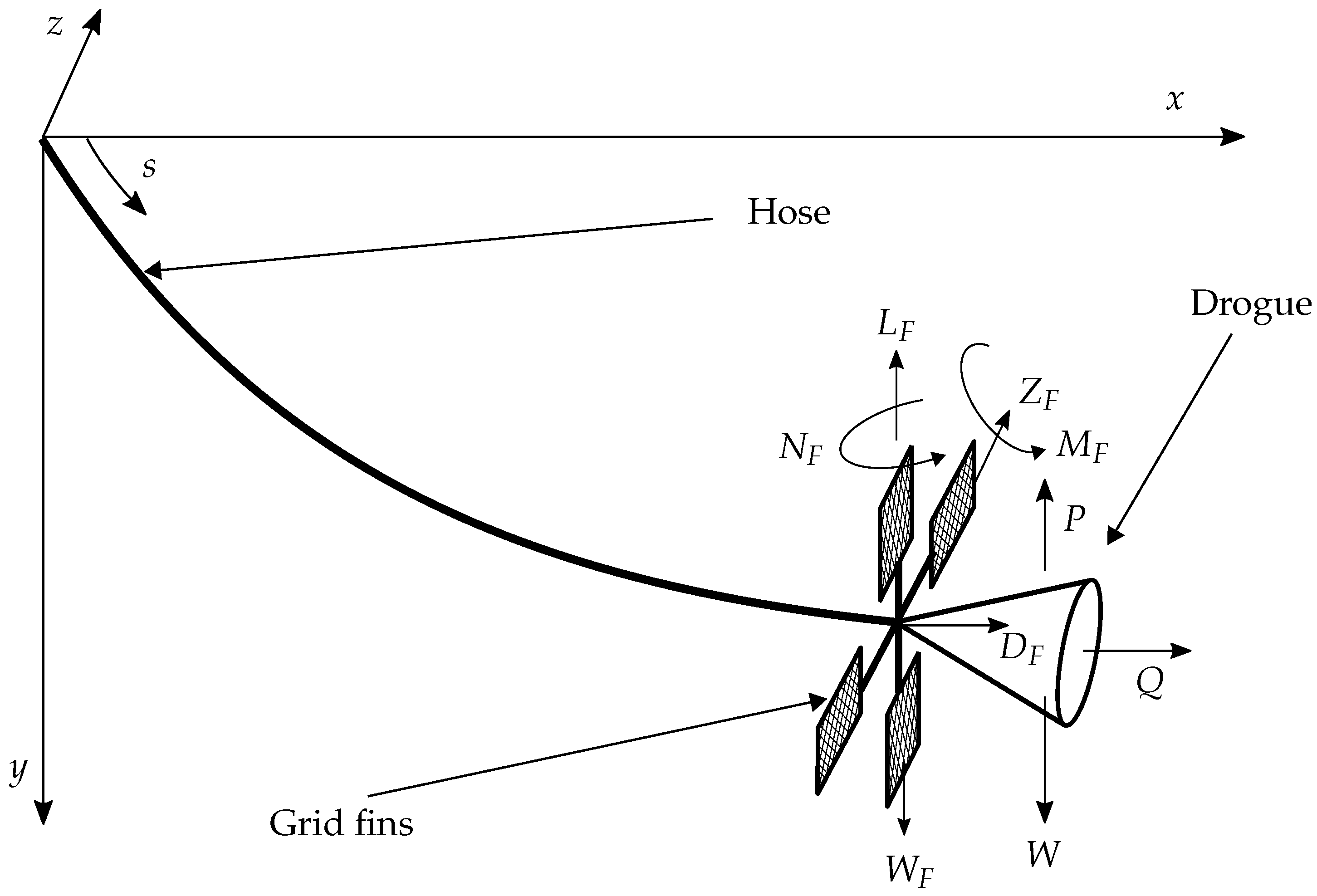
Figure 1 presents the geometry in a differential hose element, as well as at the hose–drogue–fin junction at the end of the hose. As can be seen, the reference system
is defined by the
x-axis opposite to the flight direction, the
y-axis pointing downwards, and the
z-axis forming right-handed Cartesian axes. In order to obtain the equations of the model,
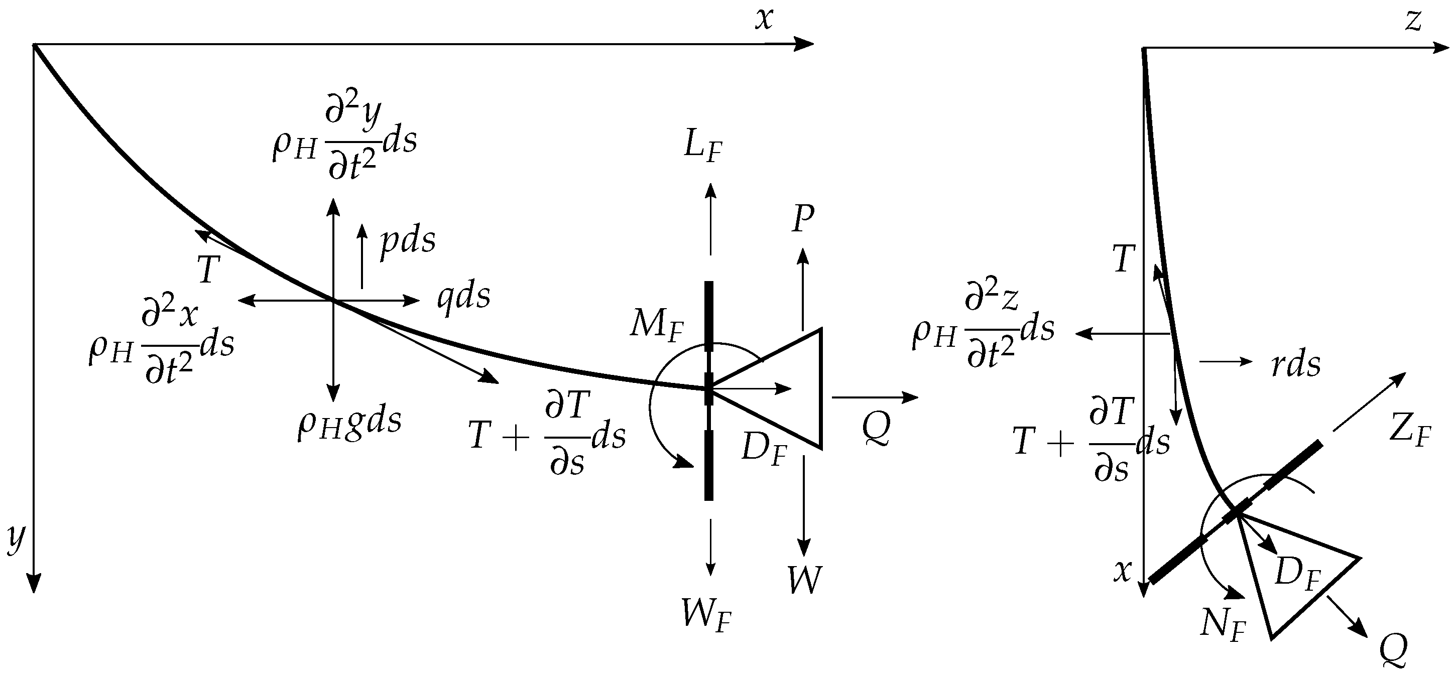
Figure 1 can be projected in a vertical plane
and in a horizontal plane
to show the acting forces in a differential hose element, as can be seen in
Figure 2.
The governing equations for the coordinates of the hose,
, and for the hose tension
, with no considerations of bending forces as a first step in the model, are as follows:
where
s is the hose arc length;
t is the time;
is the mass per unit length of the hose;
c is the structural damping coefficient of the hose;
q,
p, and
r are the drag, the lift, and the lateral aerodynamic force (all per unit length) on the hose; and
is the downwash angle induced by the tanker wake. The results obtained for the hose and drogue model without grid fins showed that, in general, the configuration will be symmetrical with respect to the
plane. Ro and Kamman [
18] have shown that, even for the case of asymmetry of the hose–drogue system with respect to the wing location, the lateral deviation is small. Therefore, in our configuration with grid fins, as will be shown in
Section 3, the lateral force on the hose,
r, will be very small and can be neglected.
The drag and the lift on the hose can be written following [
13], as follows:
where
and
are defined following the work of [
19]:
where
is the hose external diameter,
is the friction drag coefficient, and
is the zero-lift drag coefficient.
The boundary conditions of Equations (1)–(4) at the hose–tanker junction,
, are as follows:
where
,
, and
represent the prescribed motion at the hose–tanker connection. Equations (9)–(11) must be completed with geometric or kinematic boundary conditions on the derivatives of the variables at
as a function of the considered case of the connection (for example, pinned, clamped, etc.). On the other hand, the boundary conditions at the hose–drogue–fin junction,
, are as follows:
where
is the total hose length;
W is the drogue weight;
P and
Q are the drogue lift and drag, respectively;
is the grid fin weight (
is the weight of the complete system, drogue+grid fins);
is the grid fin lift;
is the grid fin drag; and
is the grid fin side force.
Starting from an initial static equilibrium position, the system is perturbed with a small amplitude. Hence, the four variables of the system can be expressed as follows:
where
,
,
, and
are the static equilibrium coordinates of the system and the static hose tension;
is the small amplitude unsteady perturbation parameter; and
,
,
, and
are the perturbed values of the variables. With respect to
, the work of [
20] shows that is not affected by unsteady effects (see also, for example, [
8]). Therefore, the unsteady hose tension has been assumed to be negligible. Additionally, the angle of attack of the hose can be divided in two different terms:
where
is the steady angle of attack and
is the unsteady angle of attack. The steady angle can be expressed as a function of the static unknowns by projecting in both axes:
As can be seen in Equations (20) and (21), the steady angle of attack includes the effect of the downwash angle induced by the tanker aircraft
. The modeling of this angle is performed using the Lifting Line Theory. This angle affects the steady angle of attack
and, due to the coupling between the steady and the unsteady motion (see
Section 4), will also influence the dynamics of the system.
With respect to
, considering the unsteady effect due to the motion of the system and assuming small angles, it can be expressed as the ratio of the vertical speed of the hose
to the free-stream speed
:
By projecting the angle of attack onto both axes and linearizing it, the aerodynamic forces on the hose (Equations (5) and (6)) can also be split into a steady term and a term of order
:
Regarding the steady problem, a numerical integration of the resulting nonlinear system of equations yields the static equilibrium position of the system and the static tension of the hose. Afterwards, the dynamic problem, i.e., the system of equations to be obtained with the perturbed variables from Equations (15)–(17), must be resolved.
3. Grid Fin Prototype. Aerodynamic Characterization
As mentioned in
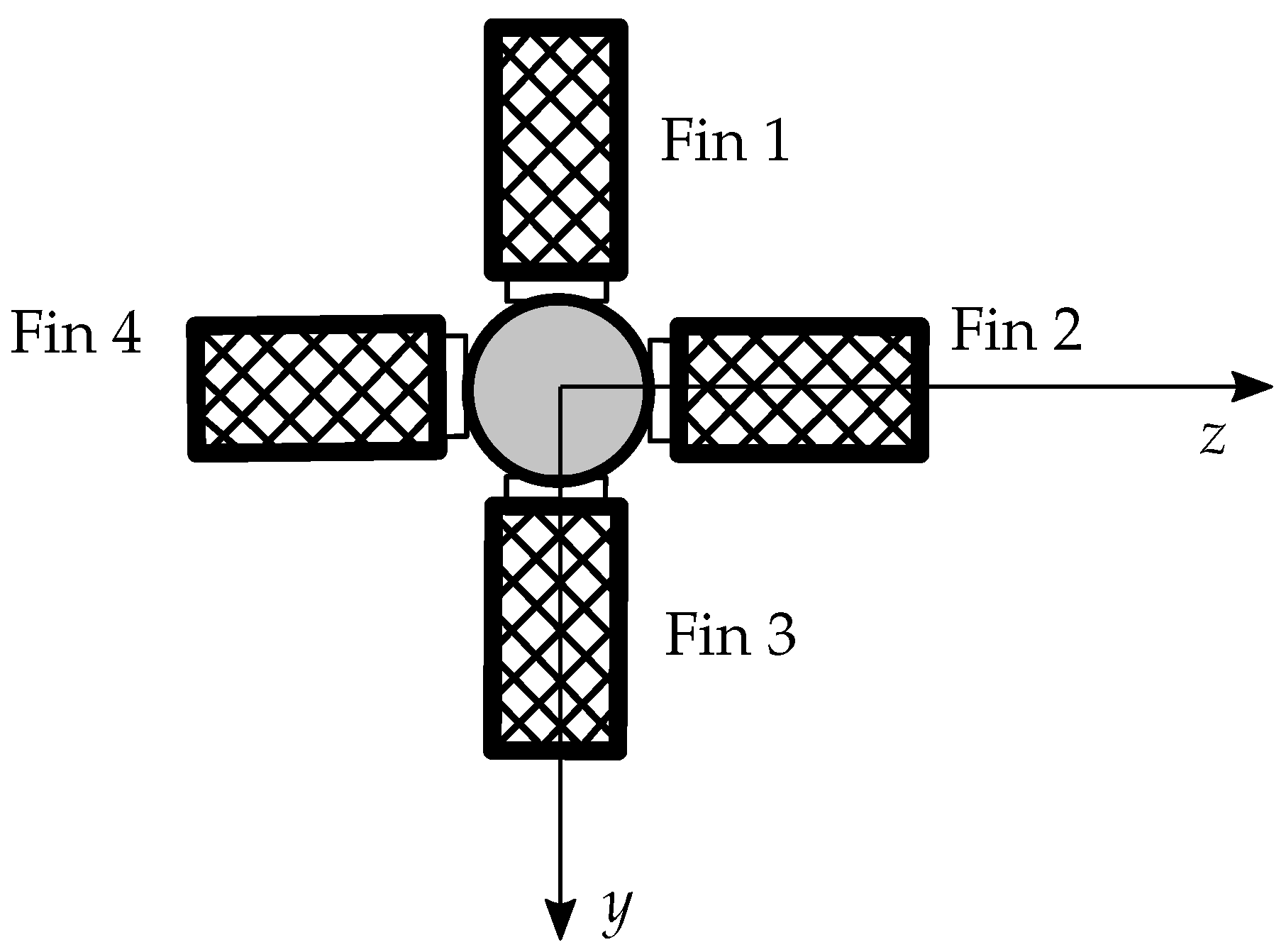
Section 1, in order to provide automatic control stabilization when the receiver approaches the drogue, a grid fin prototype is included at the end of the hose. The configuration of the prototype is shown in
Figure 3.
As can be seen, there are two fins in vertical position (fins 1 and 3) and two fins in horizontal position (fins 2 and 4). Each of these fins can rotate around its own axis independently of the drogue. These motions, together with the motion of the complete model in the hose–drogue–fin junction (pitch and yaw) will allow for defining a local angle of attack (rotation around the z-axis) and a local angle of sideslip (rotation around the y-axis) of each of the fins and , for .
With the addition of the grid fin aerodynamic forces, as seen in Equations (12)–(14), the static and dynamic behavior of the whole system will be altered. The method to obtain the aerodynamic forces on the grid fins is based on the work of [
17], generalized in order to include the unsteady motion of the grid fins. In this reference, the complete fin was divided into unit grid fins (UGF). On each UGF, the aerodynamic forces were computed. Multiplication of the net forces acting on each UGF by the number of total equivalent UGF provided the total force on the fin. In [
17], it was shown that the comparison of the results by the simplified UGF method and the solution of the complete fin is very accurate in the subsonic regime. While in this reference, the solution of the complete fin was achieved using a CFD code, in this work, the aerodynamic coefficients will be obtained with the Doublet-Lattice Method (DLM) code. With this code, a UGF normal force coefficient
is calculated as a function of the Mach number
and for the reduced frequency of the unsteady motion of the system
. With the approach of the UGF method, the lift coefficient slopes on the vertical and horizontal fins can be expressed as follows:
where
is the reference surface of a UGF;
is the reference surface of a complete fin; and
and
are the equivalent UGF for a vertical and an horizontal fin, respectively, which are estimated following the same procedure described in [
17]. It is important to point out that, due to the symmetry of the fin configuration, the side force coefficient slopes in the fins can be obtained easily from the lift coefficients:
and
. Once
and
have been obtained, it is possible to develop a formulation to calculate the aerodynamic forces on the complete fins. Contributions to the total forces, such as the interference terms between the four fins and the rest of the prototype, are obtained from experimental data, while the computations from the DLM are strictly associated with the isolated fins. Although these other contributions are always very small with respect to the fins themselves, they are included in the results used for the aerodynamic coefficients.
For the configuration presented in
Figure 3, the lift and the side force coefficient for each grid fin are as follows:
for
. The complete coefficients can be obtained from Equations (27) and (28):
where
and
are correction factors needed to include interferences and other effects obtained from experimental data. With respect to the rest of the aerodynamic coefficients, the drag coefficient
is obtained from experimental data of static tests. Therefore, it will be assumed completely steady, i.e., in the perturbed equations, it will not appear. The pitch and yaw moment coefficients
and
are obtained in a similar way to Equations (29) and (30). However, since they will have no effect on the results (the bending and torsion of the hose are not considered in the model), these expressions are not included in this development. Once the aerodynamic coefficients are known, the grid fin forces can be expressed as follows:
In a similar way to Equations (15)–(18), the angles of attack and sideslip of the grid fins can be split into a steady and in an unsteady contribution (for a symmetric case of the grid fin configuration):
where
and
are the steady angle of attack and sideslip of each fin, and
and
are the unsteady angle of attack and sideslip of each grid fin (
). Thus, Equations (27) and (28) can be rewritten as follows:
Linearizing and retaining only terms of order
, the unsteady force coefficients
and
are as follows:
The coefficients
and
for the total forces are obtained with Equations (29) and (30). It can be seen that both coefficients
and
are functions of eight unknowns: the unsteady angles of attack
and sideslip
of each of the four fins. It is possible to write these two expressions in matrix form as a function of the unknowns:
, where the vector of unknowns will be the following:
Additionally, the matrix is as follows:
where each coefficient of the matrix can be defined, following Equations (38) and (39), as follows:
for
. Equation (
41) gives the generalized unsteady force matrix of the fins as a function of their angles of attack and sideslip. To couple the aerodynamic forces on the fins with the dynamic equations on the hose, this matrix must be expressed as a function of the three perturbed variables of the dynamic problem:
,
and
. By analyzing the fin angles at the static equilibrium position, a relationship between these angles and the static variables can be found:
where it has been assumed that the angles in the hose–fin–drogue junction are small. In Equation (47), it can be observed that the value for
is very small, and therefore, the lateral forces on the hose can be neglected. Starting with fin 1, once the system is perturbed from their static position, the unsteady angles of attack and sideslip could be written, retaining terms of order
, as follows:
Using the relationships of Equations (46) and (47), the angles of attack and sideslip of fin
i can be expressed as a function of the perturbed variables of the system at the hose–drogue–fin connection (
):
for
. Equations (50) and (51) can be written as a transformation matrix
between the grid fin angles and the derivatives of the perturbed variables. With this transformation matrix, the unsteady aerodynamic force matrix of the fins as a function of the unknowns is accomplished:
It should be noted that represents the dimensionless force coefficients on the fins. When added in the complete model, they will be multiplied by the dynamic flight pressure and the reference surface of the unit grid fins .
4. Unsteady Problem
With the linearization proposed in Equations (15)–(18), a PDE system of equations is obtained, where the unknowns are the perturbed variables of the system:
Additionally, the boundary conditions are as follows:
where
is the unsteady grid fin force coefficients obtained from Equation (
52). Applying separation of the variables, the perturbed variables of the system can be expressed as follows:
An improved model for the unsteady aerodynamic forces acting on the hose can be obtained by adding a phase lag angle between the acting unsteady aerodynamic forces on the hose and the hose dynamic motion. This phase lag angle
will be introduced through the unsteady angle of attack and will affect the dynamic motion of the system:
Just as in the cases of stall flutter events (see [
21]), in this work, the phase lag angle will be introduced in the system as one more parameter for flutter computation. The estimation of
for different flight conditions can be obtained following the work of [
22], as follows:
where
is the first frequency in a vacuum of the system and
is the first frequency of the system including the fluid effect. Therefore, once the frequencies of the system (which will be obtained solving the dynamic problem) are known, the estimation of
can be performed with this simplified expression.
With these considerations, Equations (54) and (55) can be rewritten as follows:
Additionally, the boundary conditions can be written as follows:
Equations (65)–(67) are solved using the Weighted Residual Method (see [
23]), where the spatial parts of the perturbed variables
,
and
will be approximated by form functions
. Thus, the problem formulation can be finally written in a compact matrix form as follows:
where
M,
B, and
K are the inertia, damping, and stiffness matrices, respectively;
Q is the grid fin force coefficient matrix; and
u is the vector that represents the degrees of freedom of the system (the horizontal, vertical, and lateral displacements of the system). Considering the different contributions, the inertia matrix can be expressed by the following sub-matrices:
where
,
, and
are the inertia matrices of the horizontal, vertical, and lateral motions of the hose, respectively. The damping matrix can be written as follows:
where
and
are the damping matrices of the horizontal and the vertical motion, which will have aerodynamic and structural contributions, and
is the horizontal damping term due to the vertical motion. In this matrix, there is a coupling between vertical and horizontal motion, as shown in Equation (
65). Concerning the lateral motion of the hose, it has no aerodynamic damping (a fact that can be seen in Equation (67)). For that reason,
terms come only from the structural damping
c. With respect to the stiffness matrix, it can be written as follows:
where
,
, and
are the stiffness matrices of the horizontal, vertical, and lateral motions of the hose, and
is the coupling that appears in the horizontal stiffness matrix due to the vertical motion.
As can be seen both in the equations and in the resulting matrices, coupling terms between horizontal and vertical motion appear in
B and
K. However, these terms are only seen in the horizontal motion (Equation (
65)), while they do not appear for the vertical one (Equation (66)). Therefore, the horizontal motion is coupled with the vertical motion, but not vice-versa, which implies that it is possible to solve the vertical motion of the system independently of the horizontal one. Furthermore, it can be noticed that the lag angle
will appear in the aerodynamic contributions of
B and
K (for more details, see [
24]).
The grid fin force matrix is formed using the following sub-matrices:
As seen throughout the development of the formulation, the terms associated with the fin forces only appear for the boundary conditions at the hose–drogue–fin connection (
). Therefore, the sub-matrices of Equation (
76) can be defined as matrices of zeros except in the terms corresponding to this node:
where
,
,
N represents the position of the hose–drogue–fin junction in the matrix and
is the different terms that show up in the grid fin aerodynamic matrix defined in Equation (
52).
5. Flutter Analysis
The main purpose of this work is to analyze the aeroelastic behavior of the hose–drogue–grid fin system by obtaining the flutter boundaries under different flight conditions and values of the parameters. It is important to highlight that the system can be considered statically nonlinear but dynamically linear, being coupled static and dynamic problems. Therefore, the nonlinear static equilibrium position will affect the dynamic forces, unlike the classical flutter computation (see, for example, [
25]). In other words, the flutter solution will be influenced by nonlinearity effects of the static configuration equilibrium. In [
24], an overview for the flutter computations of this type of systems is explained. However, in this work, one of the main novelties is the inclusion of the grid fin prototype in the hose–drogue model. Thus, another important goal is to analyze the effect of the grid fins in the aeroelastic behavior of the system. Flutter analysis will be performed by means of the k-Method (see [
26]). Assuming harmonic motion
, Equation (
72) can be rewritten as follows:
The aerodynamic force matrix is henceforth expressed as a function of the Mach number
and the reduced frequency
k, since the grid fin aerodynamic coefficients are a function of these parameters. As usually performed in this type of analysis, in order to reduce the number of modes of the system, a modal approximation is introduced:
where
is the modal matrix of the conservative system, the columns of which include the low-frequency modes, and
is the vector of modal coordinates considered. Pre-multiplying by
gives
Following the k-Method, a fictitious damping coefficient
g proportional to the displacement is introduced:
dividing by
g and grouping the generalized mass matrix and the grid fin force matrix,
After manipulation of the different terms, Equation (
83) can be written as a explicit function of the flight speed:
where the reduced frequency is written as
, with
being the chord of the grid fins. The eigenvalue of Equation (
84) is as follows:
which can be approximated by
Procedure
The procedure to obtain the flutter boundaries in the hose–drogue–grid fin system will be the following:
The configuration of each grid fin (and therefore the values of the angles and ) are selected.
The flight Mach number is fixed.
The flight altitude , and, therefore, the speed of sound and the air density are fixed. The flight speed is , and the dynamic pressure is .
The static equilibrium position of the system at the flight speed and the flight altitude is obtained.
From the steady position:
- (a)
Mass, damping, and stiffness matrices of the systems M, B, and K are computed.
- (b)
With M and K, the modal matrix of the conservative problem is , and therefore, the generalized matrices , , and are obtained. Matrix will, in general, not be diagonal, while matrices and will.
A range of interests of the reduced frequency is selected. For each reduced frequency :
- (a)
The unsteady force coefficient from the UGF Method is computed. Then, the unsteady grid fin force matrix Q is obtained, and with , the generalized matrix is .
- (b)
The eigenvalues of Equation (
84) for each mode
are computed. Then, we obtain
The flutter speed ;
The damping ;
The frequency .
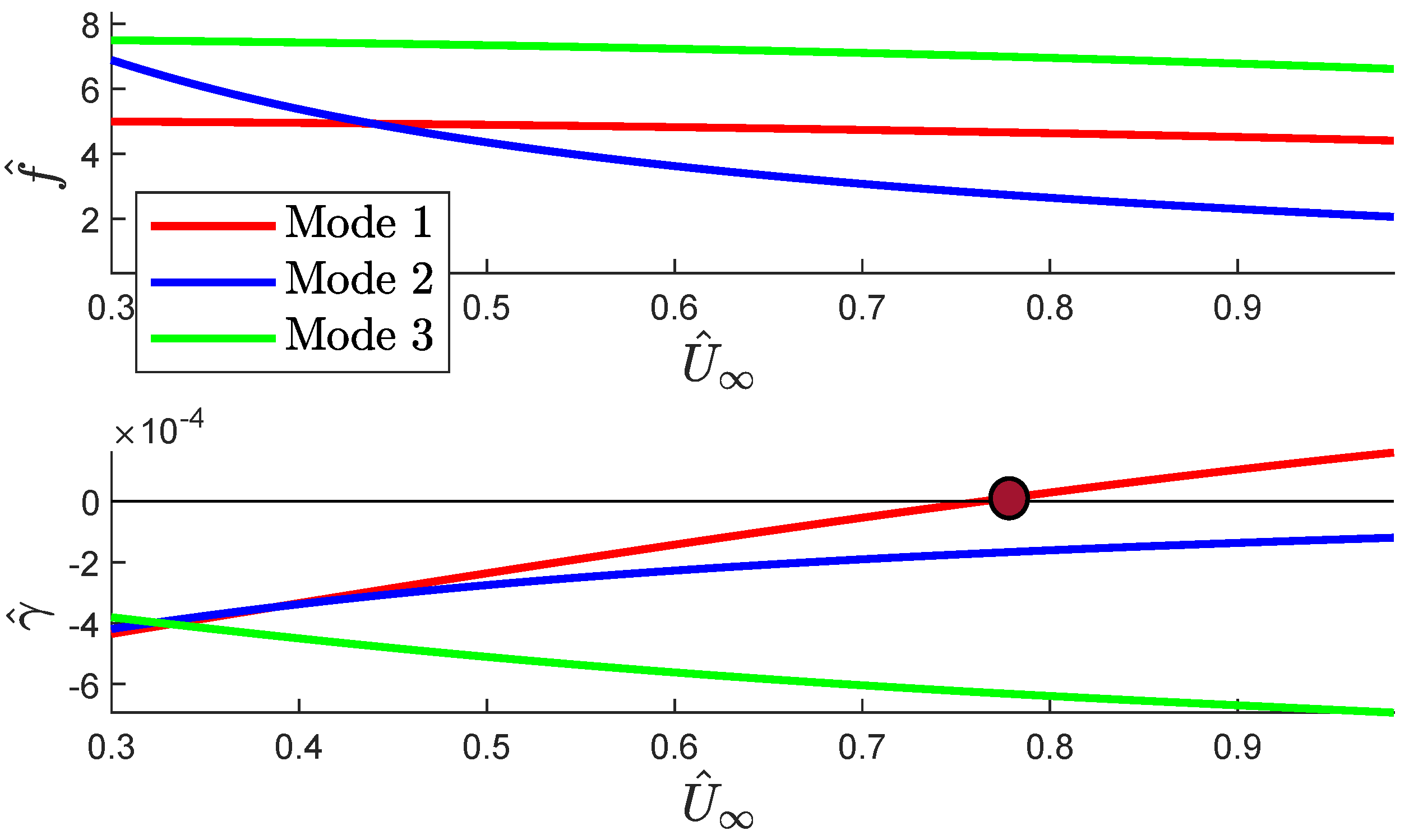
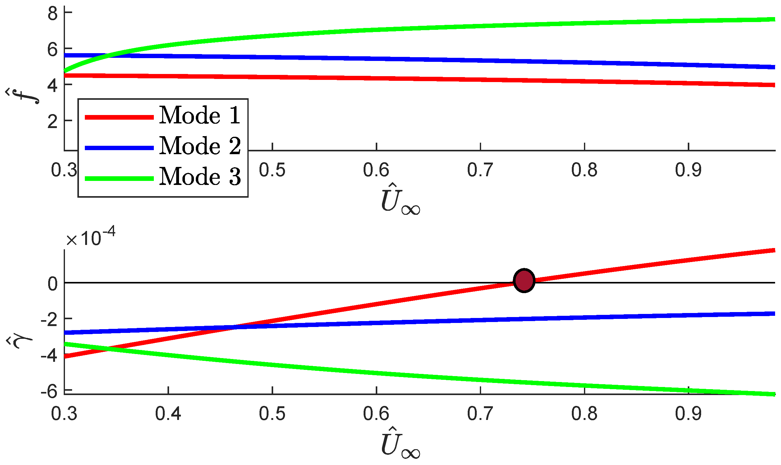
diagrams, representing and , are sketched.
The flutter speed will be the lowest at which any of the damping coefficients becomes positive. From the diagram at this speed, the flutter frequency is obtained.
7. Conclusions
The aeroelastic stability of a hose–drogue system with an aerodynamic grid fin model has been presented. Starting from the steady configuration of the complete system, a time linearization was performed in order to obtain the dynamic system of equations and to subsequently analyze the aeroelastic behavior.
A prototype of grid fins was included in the model with the aim of increasing the stability of the system during the refueling process. An efficient method to obtain the aerodynamic forces of the grid fins was developed.
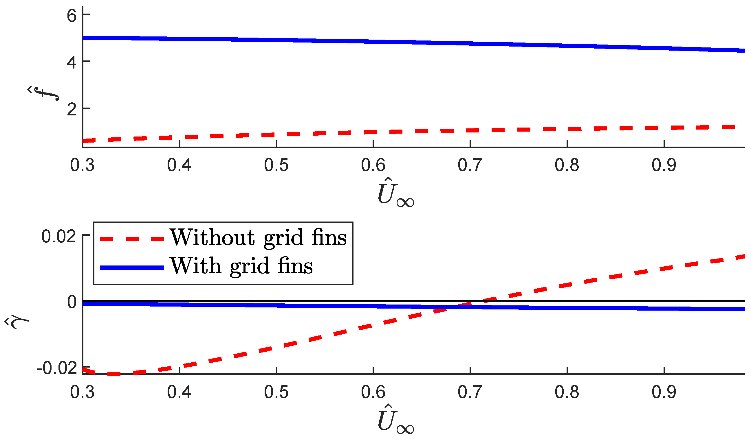
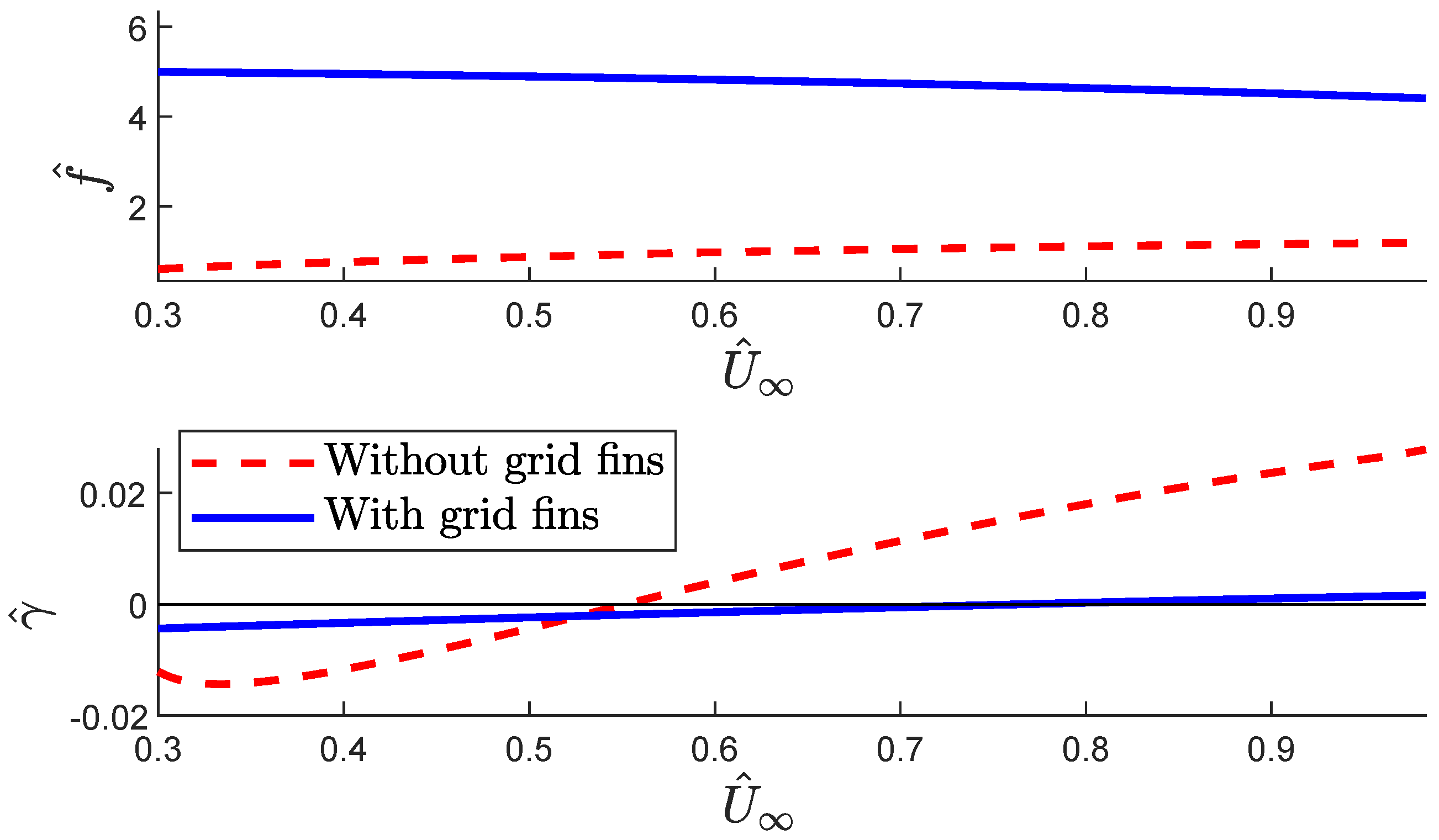
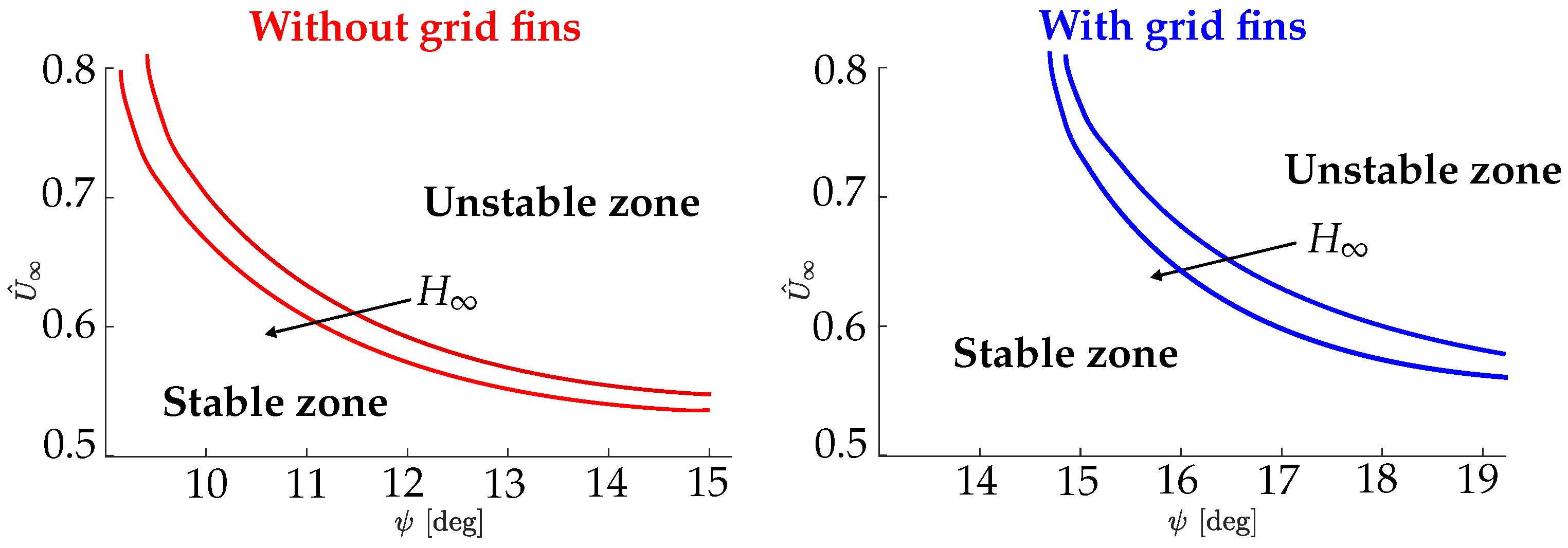
The possibility of flutter in the complete system was studied by means of the k-Method. The results were obtained from different flight conditions and values of the phase lag angle between the unsteady aerodynamic forces on the hose and the hose motion. These results were compared with the ones obtained without the grid fin model. It was shown that the inclusion of the grid fins produces a significant increase in the aeroelastic stability of the ensemble: flutter without grid fins appears for a phase lag angle around 10°, while that with grid fins is delayed to 15°. Likewise, the same type of aeroelastic instability (one degree-of-freedom flutter) as in the case without grid fins was obtained, as was the same flutter mechanism (the first mode of the system). It was also found that results have a smooth variation with the flight altitude.
This work will continue with an analysis of different configurations of the grid fins (for example, cross configuration). Furthermore, the addition of the bending forces on the hose and the tanker wake using a vortex lattice method will complete the model for linear analysis. In this way, the hose–drogue–grid fin system will be able to analyze the most stable ensemble for an aerial refueling process.


