Generation of Guidance Commands for Civil Aircraft to Execute RNP AR Approach Procedure at High Plateau

Abstract

RNP AR is an operational procedure that uses the aircraft’s airborne navigation equipment and global positioning system to guide the aircraft to take off and land, and it is an effective means to ensure the flight safety of civil aircraft at high-plateau environments. In this paper, a three-dimensional, precise guidance command generation method for performing an RNP AR approach procedure is proposed. The lateral navigation transition paths between different segments are constructed, and a lateral segment switching strategy based on the angular bisector is introduced. To illustrate the availability of the proposed algorithm, a simulation based on the RNP AR approach procedure of Jiuzhai Huanglong Airport is operated, and it can be drawn from the results that the proposed algorithms can provide lateral and vertical guidance capabilities that meet the requirements of RNP AR approach.

1. Introduction

High-precision terminal operation at high-plateau airports is a worldwide challenge, especially for China’s civil aviation transportation industry [1]. A high-plateau airport refers to an airport with an altitude of more than 8000 feet (about 2438 m), which has low air density and atmospheric pressure, complex and harsh terrain, poor airport clearance, and so on [2]. These special environmental characteristics make it more difficult for airliners to take off and land. Due to the limitations of the complex geographical environment, airliners are required to adopt required navigation performance with authorization required (RNP AR) flight procedures when operating at high plateau airports.

RNP AR is a flight procedure that uses the airborne navigation equipment and global positioning system (GPS) to guide aircraft to take off and land [3,4]. RNP AR can realize the required navigation accuracy, integrity, availability, and continuity, and can achieve the monitoring and alarm of actual airborne navigation performance [5].

The RNP AR approach procedure is a high-performance RNP procedure, which is of great value for ensuring take-off and landing safety of civil aircraft at high-plateau airports or some special airports [6,7]. The advantages of RNP AR can be summarized as follows: ① It can effectively reduce the impact of obstacles via a flexible horizontal trajectory to increase the take-off weight [8]. ② Precise flight guidance can improve the airspace capacity and efficiency and reduce fuel consumption and exhaust emissions [9,10,11]. ③ As with RNP operations, it can reduce the workload of the crew [12] and increase the operational benefits [13]. ④ The RNP AR approach procedure supports a curve approach, and it can be applied in combination with fixed glide angle approach methods such as the instrument landing system (ILS) and FMS landing system (FLS) to achieve better performance [14,15]. Due to the limitations of the complex terrain environment, the aircraft is required to track the desired trajectory with high accuracy when performing the RNP AR approach procedure. Therefore, how to generate three-dimensional (3D) precise flight guidance commands is an important issue.

At present, there is no specific configuration of flight guidance law for each type of segment in public documents due to trade secrets or other reasons. In this paper, a flight guidance command generation method for civil aircraft to perform the RNP AR approach procedure is proposed, and the contributions are summarized as follows:

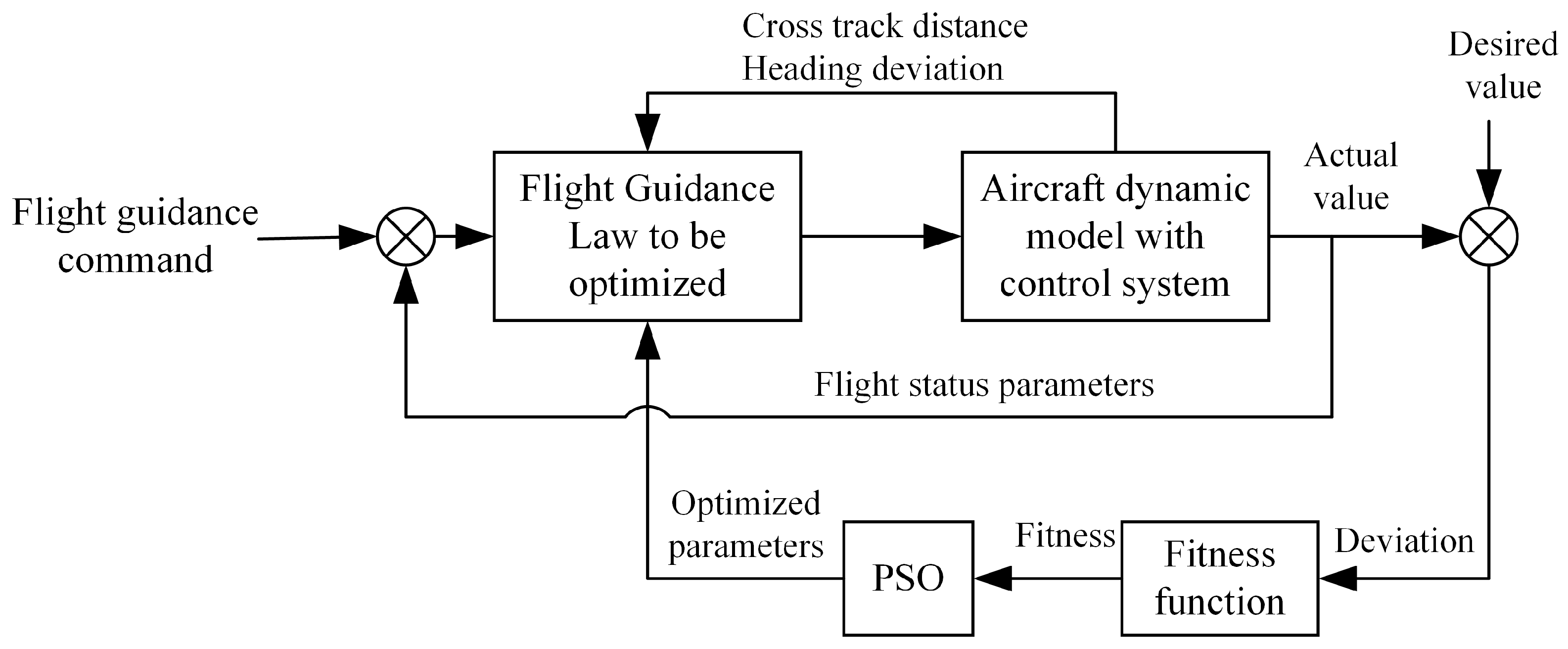
• A 3D precise guidance command generation method for civil aircraft to perform the RNP AR approach procedure is proposed. Specifically, the lateral flight guidance law is designed based on the guidance requirements of the horizontal segment, and the vertical guidance commands are calculated according to the type of the horizontal segment. In addition, a flight guidance law parameter-tuning strategy based on the particle swarm optimization algorithm is given.
• The construction method of the lateral navigation transition paths in ARINC specification 424-21 is presented, including tangent transition, position interception, 45° interception, direct transition, and arc interception. Furthermore, a lateral segment switching strategy based on the angular bisector is introduced to realize automatic flight, and the implementation process of the proposed method is described in detail.
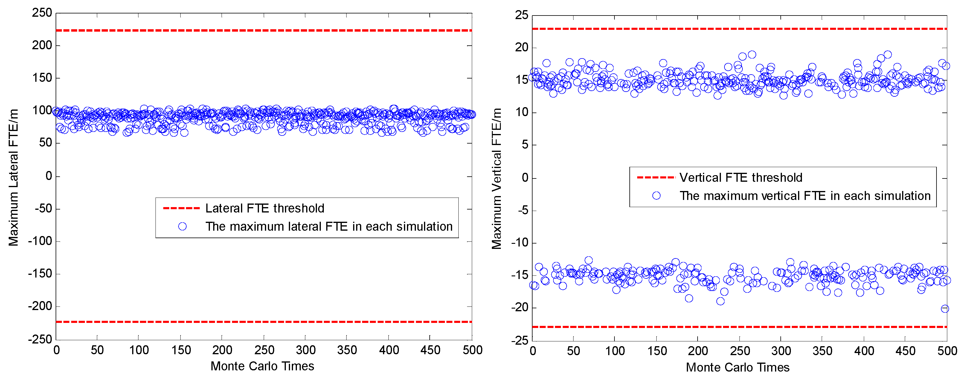
• To verify the effectiveness of the proposed algorithm, based on analyzing the RNP AR approach guidance requirements of Jiuzhai Huanglong Airport, the flight technical error (FTE) is selected as the index to evaluate the guidance effect of the proposed guidance algorithm, and 500 stochastic simulations are conducted via the Monte Carlo method under navigation sensors for noise and wind disturbance.

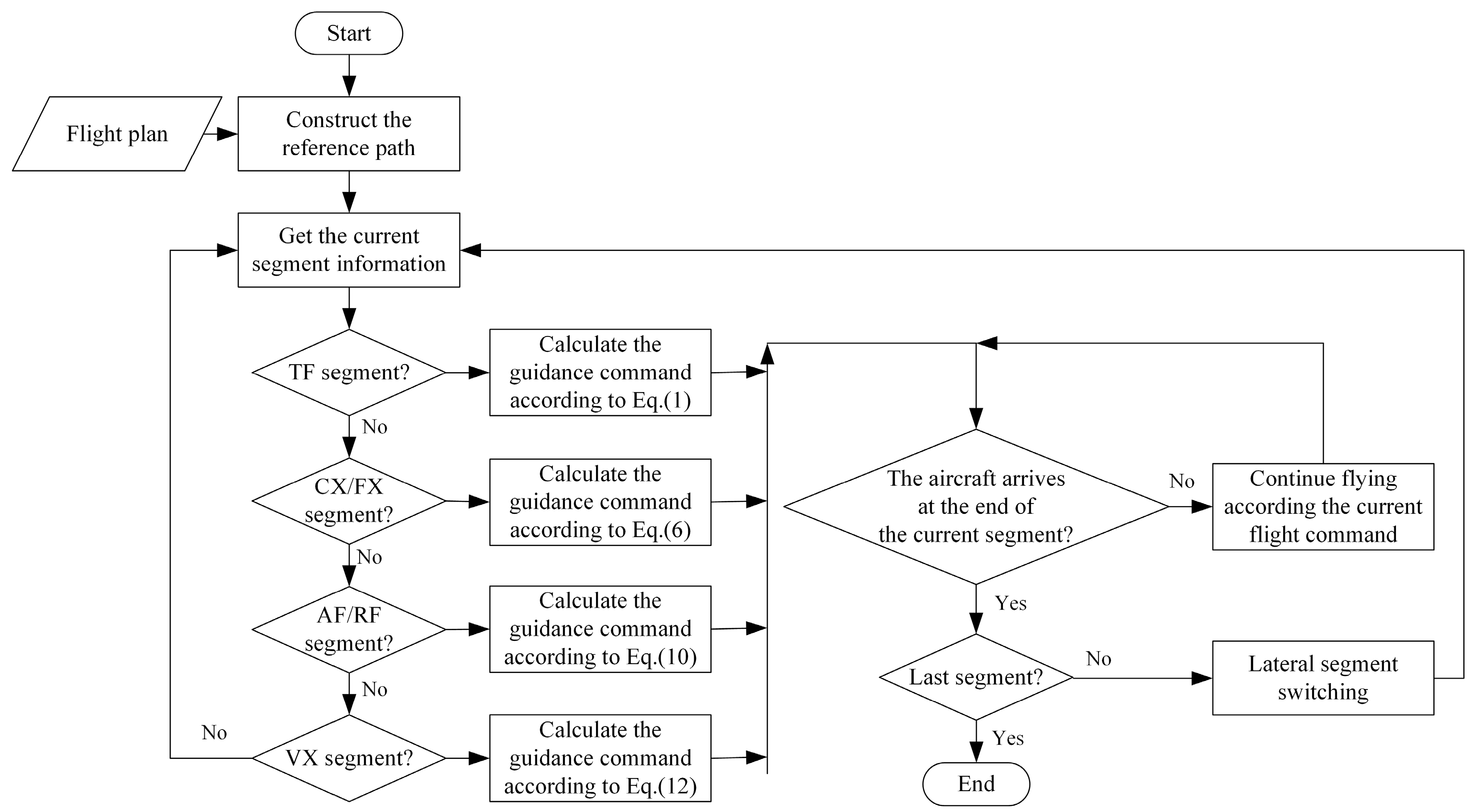
2. Design of Guidance Law for Performing RNP AR Approach Procedure

The 3D precise guidance commands consist of lateral guidance command and vertical guidance command. Therefore, it is necessary to design lateral guidance law and vertical guidance law for civil aircraft to perform the RNP AR approach procedure according to the segment characteristics.

2.1. Design of Lateral Flight Guidance Law

There are 23 types of lateral segments in ARINC specification 424-21 [16], which are the basis of the horizontal trajectory of the RNP AR approach procedure.

Referring to the guidance requirements of each type of segment, the 23 types of lateral segments can be divided into four categories according to the segment characteristics, and they are TF segments, CX and FX segments, AF and RF segments, and VX segments. The involved segment types are shown in Appendix A, and the lateral flight guidance laws are designed as follows:

(1)

TF segment

The TF segment is a great circle route, which is defined by the starting point $P_1(L_1,{\lambda }_1,h_1)$ and the ending point $P_2(L_2,{\lambda }_2,h_2)$, and the spatial position is determined, where $L$ is the latitude, $\lambda$ is the longitude, and $h$ is the altitude. The azimuth angle of the TF segment is unequal everywhere, so the guidance law of the TF segment is given as Equation (1).

$${\varphi }_c=k_d\cdot \Delta D+k_{ds}\cdot \Delta \dot{D}$$

(1)

where ${\varphi }_c$ is the desired roll angle, and $\Delta D$ is the cross track distance (XTK). $k_d$ and $k_{ds}$ are the gains.

If the current aircraft position is $P(L,\lambda ,h)$, then $\Delta D$ can be calculated by

$$\Delta D=\left(R_L+h\right)\arcsin \left({\mathit{u}}_P\mathbf{·}{\mathit{u}}_{P_1{P}_2}\right)$$

(2)

where $R_L$ is the earth radius, and $u_P={\left[\cos L\cos \lambda ,\cos L\sin \lambda ,\sin L\right]}^T$, ${\mathit{u}}_{P_1{P}_2}$ can be expressed as

$${\mathit{u}}_{P_1{P}_2}=\frac{{\mathit{u}}_{P_1}\times {\mathit{u}}_{P_2}}{\left|{\mathit{u}}_{P_1}\times {\mathit{u}}_{P_2}\right|}$$

(3)

where

$${\mathit{u}}_{P_1}\times {\mathit{u}}_{P_2}=\left[\begin{array}{c}-\sin L_1\cos L_2\sin {\lambda }_2+\cos L_1\sin {\lambda }_1\sin L_2\\ \sin L_1\cos L_2\cos {\lambda }_2-\cos L_1\cos {\lambda }_1\sin L_2\\ -\cos L_1\sin {\lambda }_1\cos L_2\cos {\lambda }_2+\cos L_1\cos {\lambda }_1\cos L_2\sin {\lambda }_2\end{array}\right]$$

(4)

Then, $\Delta \dot{D}$ can be calculated by Equation (5).

$$\Delta \dot{D}=\left(R_L+h\right)\frac{d\left[\arcsin \left({\mathit{u}}_P\mathbf{·}{\mathit{u}}_{P_1{P}_2}\right)\right]}{dt}=\frac{\left(R_L+h\right)}{\sqrt{1-{\left({\mathit{u}}_P\mathbf{·}{\mathit{u}}_{P_1{P}_2}\right)}^2}}$$

(5)

(2)

CX and FX segments

CX segments include CA, CD, CF, CI, and CR segments, while FX segments include FA, FC, FD, and FM segments. Both CX segments and FX segments are straight legs, and they are defined by a fixed point $P_0(L_0,{\lambda }_0,h_0)$ and a known azimuth angle ${\chi }_{leg}$. As a result, the guidance law of CX and FX segments is given as Equation (6).

$${\varphi }_c=k_d\cdot \Delta D+k_{\chi }\cdot ({\chi }_{leg}-\chi )\cdot V_{GND}$$

(6)

where ${\chi }_{leg}$ is the azimuth angle of the segment, $\chi$ is the current azimuth angle of the aircraft, and $V_{GND}$ is the ground speed of the aircraft. $k_{\chi }$ and $k_d$ are the gains.

The calculation method of $\Delta D$ under rhumb line is different from Equation (2), and if ${\chi }_{leg}=\frac{\pi }{2}$ or ${\chi }_{leg}=\frac{3\pi }{2}$, it can be obtained using Equation (7). Otherwise, $\Delta D$ is supposed to be calculated using Equation (8).

$$\Delta D=(L-L_0)\cdot R_L$$

(7)

$$\Delta D=\left|P{P}_1\right|\cdot \cos {\chi }_{leg}=\left(\lambda -{\lambda }_1\right)\cdot R_L\cdot \cos L\cdot \cos {\chi }_{leg}$$

(8)

where $P_1$ is a point on the straight leg, and the latitude of $P_1$ is equal to the latitude of the current aircraft position. The longitude of $P_1$ can be calculated by Equation (9).

$${\lambda }_1={\lambda }_0+\tan {\chi }_{leg}\cdot \ln \left(\frac{\cos L_0\cdot \left(1+\sin L\right)}{\cos L\cdot \left(1+\sin L_0\right)}\right)$$

(9)

(3)

AF and RF segments

The AF segment and RF segment are arc legs with determined spatial position and arc radius. Thus, the guidance law of AF and RF segments is given as Equation (10).

$$\{\begin{array}{l}{\varphi }_{c1}=\arctan \left(\frac{V_{GND}^2}{g{R}_{arc}}\right)\\ {\varphi }_c=k_{sign}\cdot {\varphi }_{c1}+k_d\cdot \Delta D\end{array}$$

(10)

where $g$ is the gravity acceleration, and $R_{arc}$ is the arc radius. $k_{sign}$ is the gain, and if the turning direction of the arc segment is clockwise, $k_{sign}=1$; otherwise, $k_{sign}=-1$.

When the horizontal trajectory is AF segment or RF segment, $\Delta D$ can be calculated using Equation (11).

$$\Delta D=k_{sign}\cdot (D_l-R_{arc})$$

(11)

where $D_l$ represents the distance between the center of the arc leg and the current aircraft position, which can be calculated via the inverse solution of the rhumb line.

(4)

VX segments

VX segments are a kind of special segment, which include VA, VD, VI, VM, and VR segments. The track of VX segments is uncertain, and the crew controls the aircraft with a determined heading. As such, the guidance law of VX segments is given as Equation (12).

$${\varphi }_c=k_{\psi }\cdot \left({\psi }_{set}-\psi \right)+k_{\psi I}\cdot {\displaystyle \int \left({\psi }_{set}-\psi \right)}$$

(12)

where ${\psi }_{set}$ is the desired heading, and $\psi$ is the current heading of the aircraft. $k_{\psi }$ and $k_{\psi I}$ are the gains.

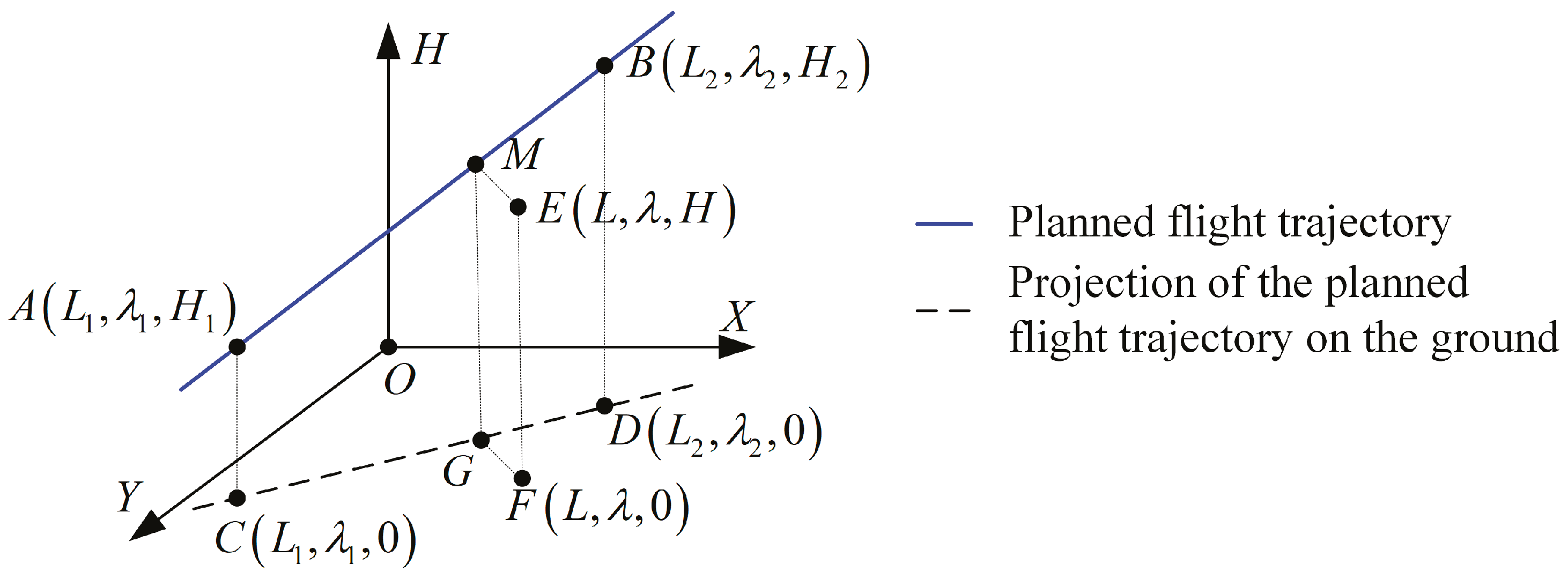
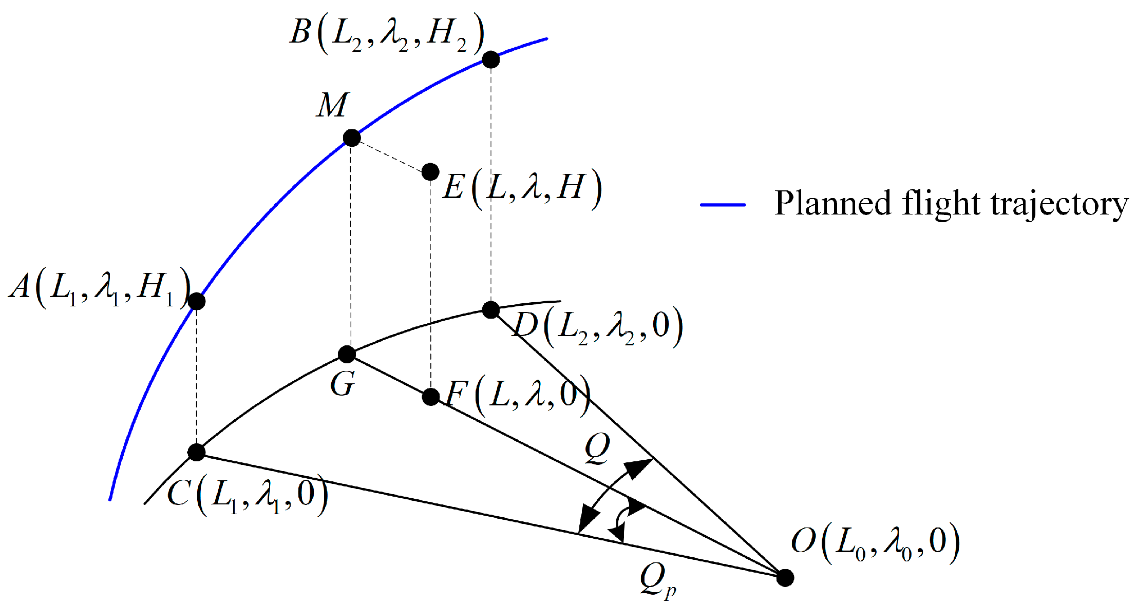
2.2. Design of Vertical Flight Guidance Law

Lateral guidance is the foundation of vertical guidance, and the horizontal trajectory can be simply divided into straight legs and arc legs.

When the horizontal segment is a straight leg, as shown in Figure 1, the starting point of the leg is $A\left({\lambda }_1,L_1,h_1\right)$, and the ending point is $B\left({\lambda }_2,L_2,h_2\right)$. $E\left(\lambda ,L,H\right)$ is the current aircraft position, and its projection on the ground level is $F\left(\lambda ,L,0\right)$. $C\left({\lambda }_1,L_1,0\right)$ is the projection of $A$ on the ground level, and $D\left({\lambda }_2,L_2,0\right)$ is the projection of $B$ on the ground level.

Calculating the length of the straight leg starting from $C\left({\lambda }_1,L_1,0\right)$ and ending at $D\left({\lambda }_2,L_2,0\right)$, and the calculation method of $D_{leg}$ is

$$D_{leg}=R\cdot \arccos (a+b)$$

(13)

where

$$\{\begin{array}{l}a=\sin (L_1)\sin (L_2)\\ b=\cos (L_1)\cos (L_2)\cos ({\lambda }_2-{\lambda }_1)\end{array}$$

(14)

Then, the desired vertical velocity can be generated using Equation (15).

$${\dot{H}}_g=\frac{\left(h_2-h_1\right)}{D_{leg}}\cdot V_{GND}$$

(15)

When the horizontal segment is an arc leg, as shown in Figure 2, the center of the arc leg is $O\left({\lambda }_0,L_0,0\right)$, and the central angle corresponding to the arc leg is $Q$. $Q_p$ is the central angle that the aircraft has already passed, and other points are defined as above.

The azimuth angle of the straight leg starting from $C\left({\lambda }_1,L_1,0\right)$ and ending at $O\left({\lambda }_0,L_0,0\right)$ can be calculated using Equation (16).

$${\chi }_1=\arctan \left(\frac{\cos (L_0)\sin ({\lambda }_0-{\lambda }_1)}{\cos (L_1)\sin (L_0)-\sin (L_1)\cos (L_0)\cos ({\lambda }_0-{\lambda }_1)}\right)$$

(16)

Calculating the azimuth angle of the straight leg starting from $D\left({\lambda }_2,L_2,0\right)$ and ending at $O\left({\lambda }_0,L_0,0\right)$, the calculation method is

$${\chi }_2=\arctan \left(\frac{\cos (L_0)\sin ({\lambda }_0-{\lambda }_2)}{\cos (L_2)\sin (L_0)-\sin (L_2)\cos (L_0)\cos ({\lambda }_0-{\lambda }_2)}\right)$$

(17)

The central angle corresponding to the arc leg can be calculated using Equation (18).

$$Q=\{\begin{array}{ll}{\chi }_1-{\chi }_2,& {\chi }_1>{\chi }_2,k_{turn}=1\\ 2\pi +{\chi }_1-{\chi }_2,& {\chi }_1\le {\chi }_2,k_{turn}=1\\ {\chi }_2-{\chi }_1,& {\chi }_1<{\chi }_2,k_{turn}=-1\\ 2\pi +{\chi }_2-{\chi }_1,& {\chi }_1\ge {\chi }_2,k_{turn}=-1\end{array}$$

(18)

In Equation (18), if the turning direction of the arc leg is clockwise, $k_{turn}=1$; otherwise, $k_{turn}=-1$.

Then, the desired flight altitude can be obtained using Equation (19).

$$H_g=h_1+\frac{Q_p}{Q}\left(h_2-h_1\right)$$

(19)

where $Q_p$ can be calculated referring to the calculation method of $Q$.

As a result, the desired vertical velocity can be generated using Equation (20).

$${\dot{H}}_g=\{\begin{array}{ll}{k}_h(H_g-H)& |{\dot{H}}_g-\dot{H}|<{\dot{H}}_{\max }\\ {\dot{H}}_{\max }& |{\dot{H}}_g-\dot{H}|\ge {\dot{H}}_{\max }\end{array}$$

(20)

where ${\dot{H}}_{\max }$ is the maximum vertical velocity limited by the aircraft performance.

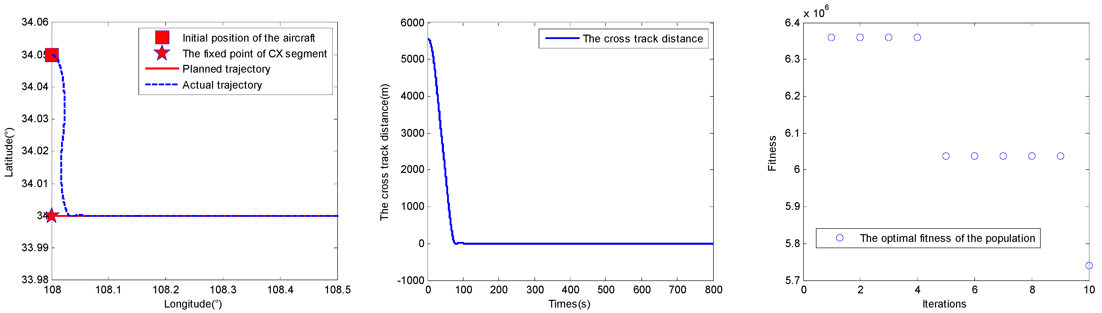
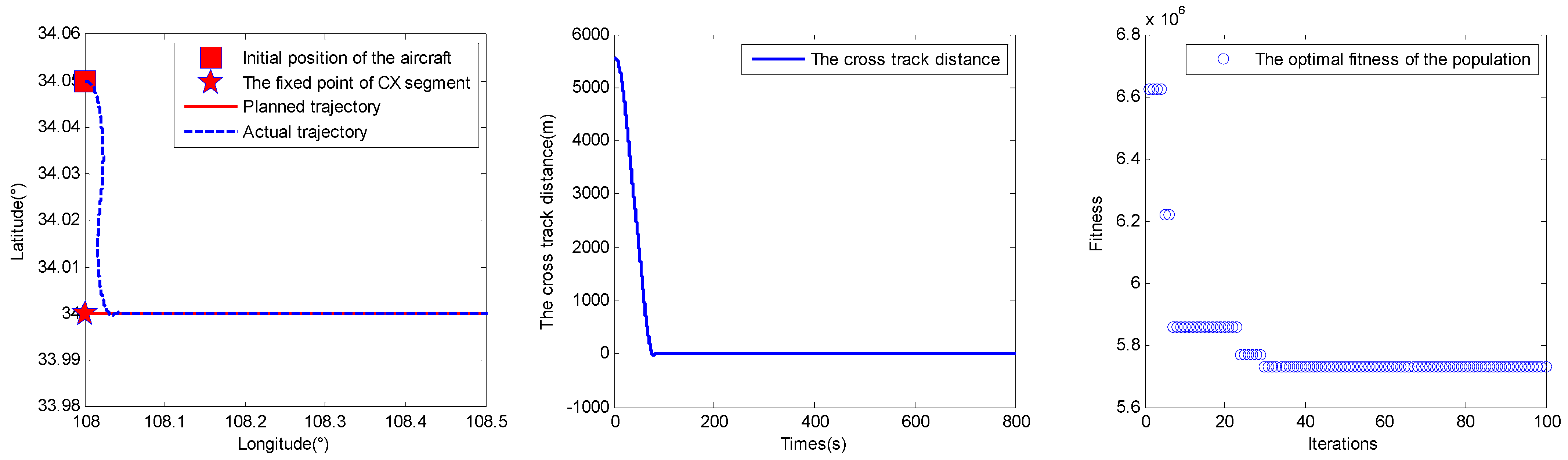
2.3. Parameter Selection of Flight Guidance Law Based on PSO

After determining the configuration of the flight guidance law, another important issue is the selection of flight guidance law parameters.

Currently, the trial-and-error method is the common parameter-tuning method. Engineers manually adjust the guidance law parameters repeatedly based on their experience until the deviation between the aircraft and the desired track meets the guidance accuracy requirements. It is undeniable that applying the trial-and-error method for parameter tuning is inefficient, and the results are not optimal.

In addition, there are large amounts of research on the application of optimization algorithms to control parameter tuning, such as particle swarm optimization (PSO), genetic algorithm (GA), ant colony optimization (ACO), and so on. Nevertheless, these studies focus on the attitude control loop rather than the track tracking loop. In this paper, the PSO algorithm is adopted to optimize the flight guidance law parameters on the basis of designed flight guidance law configuration, and the implementation principle is shown in Figure 3.

The meanings of the relevant parameters in PSO are shown in

Table 1. Symbol description in PSO algorithm.

Symbol	Variate
$N_{size}$	population size
$G_{iter}$	iterations
$X_i^j$	position of the ith particle in jth iteration
$X_{\max }$	maximum position of particles
$X_{\min }$	minimum position of particles
$V_i^j$	velocity of the ith particle in jth iteration
$V_{\max }$	maximum velocity of particles
$V_{\min }$	minimum velocity of particles
$c_1$	acceleration coefficient of the self-recognition
$c_2$	acceleration coefficient of the social
$\omega$	inertial weight
${\omega }_{\max }$	maximum inertial weight
${\omega }_{\min }$	minimum inertial weight
$f$	fitness
$f_i^j$	fitness of the ith particle in jth iteration
$f_{i,Best}$	historical optimal fitness of the ith particle
$f_{Best}$	historical optimal fitness of the population

, and the key to tuning the flight guidance law parameters using the PSO algorithm is solving the following three problems.

(1)

Encoding of feasible solutions

The coding form of feasible solutions is an important part of the PSO algorithm, and a real encoding PSO algorithm can be used to solve the problem of flight guidance law parameter tuning. The position of each particle represents a feasible solution, and the positions of all particles in the population constitute the feasible solution set. Taking the CX segment as an example, $k_d$, $k_{\chi }$, and $k_{dI}$ are the parameters that need to be tuned. Then, the ith particle can be encoded as $X=(x_1,x_2,x_3)$, where $x_1$ represents $k_d$, $x_2$ represents $k_{\chi }$, and $x_3$ represents $k_{dI}$. All particles in the population can be expressed as $X_i^j=(x_{i,1}^j,x_{i,2}^j,x_{i,3}^j)$, where $i=1,2,\cdots ,N_{size}$ and $j=1,2,\cdots ,G_{iter}$.

(2)

Construction of the fitness function

The fitness function has a crucial impact on the performance of the PSO algorithm, and it is the criterion for evaluating the quality of the feasible solution. Considering the guidance requirements of the RNP AR approach procedure, the fitness function is given as

$$f={\displaystyle \int t\left|e(t)\right|dt}$$

(21)

where $t$ is the simulation time, and $e(t)$ is the deviation between the desired value and the actual value. Then, for lateral flight guidance, $e(t)=\Delta D$, and for vertical flight guidance, $e(t)=\Delta H$.

(3)

Updating strategy

The purpose of updating is to generate a better solution on the basis of the current solution, that is, computing $X_i^{j+1}$ by $X_i^j$, where $i$ represents the index of particle, and $j$ represents the current iteration. The updating strategy of the particles can be expressed as

$$\{\begin{array}{l}{V}_i^{j+1}=\omega \cdot V_i^j+c_1\cdot r_1\cdot (P_i-X_i^j)+c_2\cdot r_2\cdot (BestS-X_i^j)\\ X_i^{j+1}=X_i^j+V_i^{j+1}\end{array}$$

(22)

where $r_1$ and $r_2$ are the uniformly distributed random numbers within interval [0, 1]. $P_i$ represents the optimal solution of the ith particle, and $BestS$ represents the optimal solution of the population.

Additionally,

$$\omega ={\omega }_{\max }+\frac{{\omega }_{\min }-{\omega }_{\max }}{G_{iter}}j$$

(23)

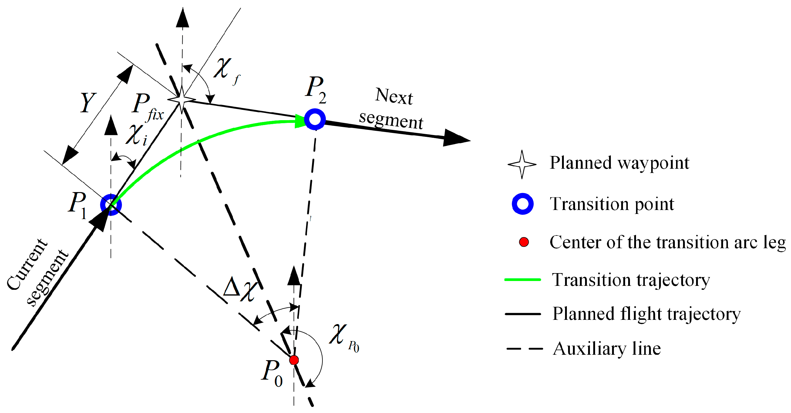
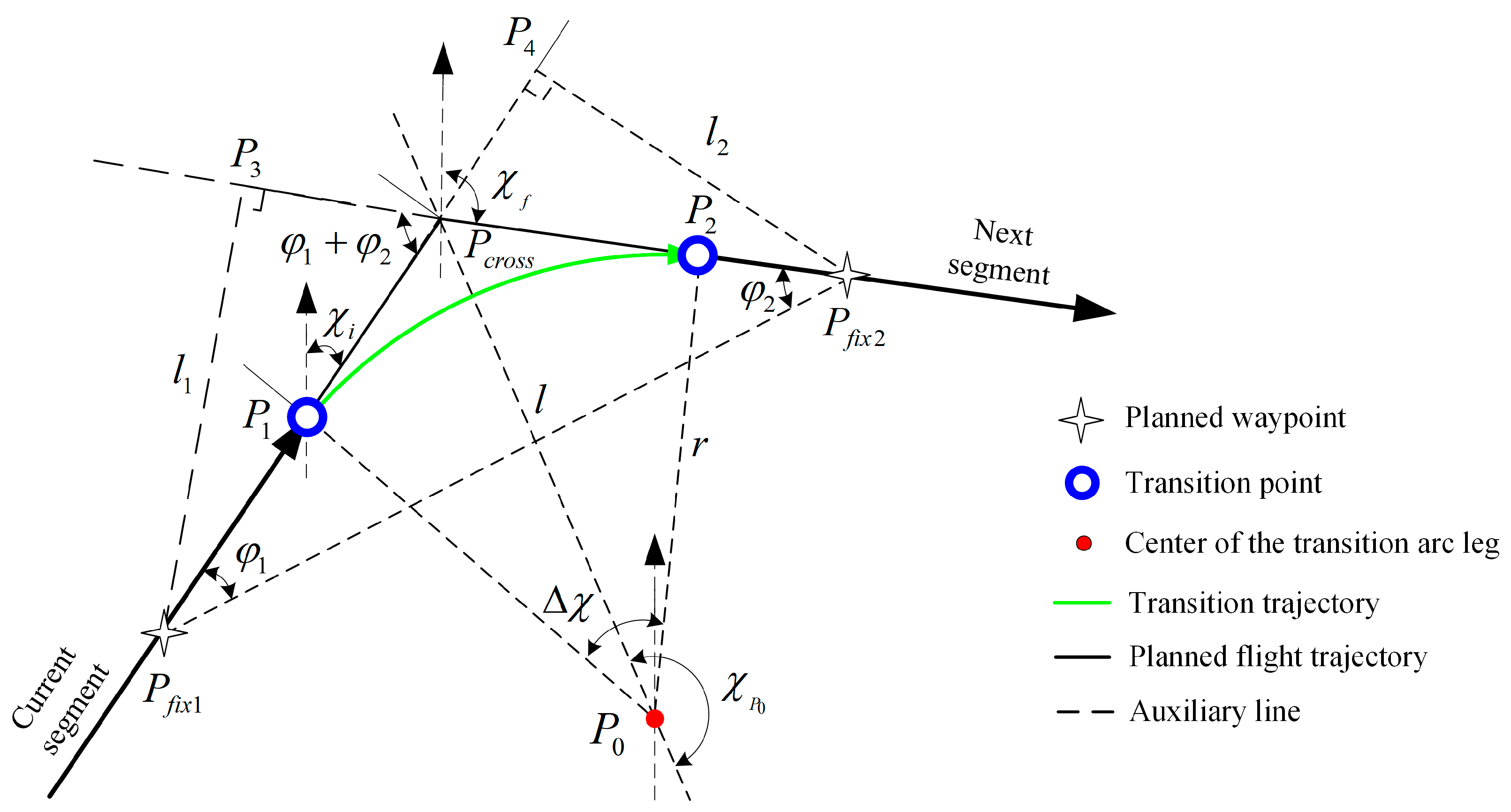
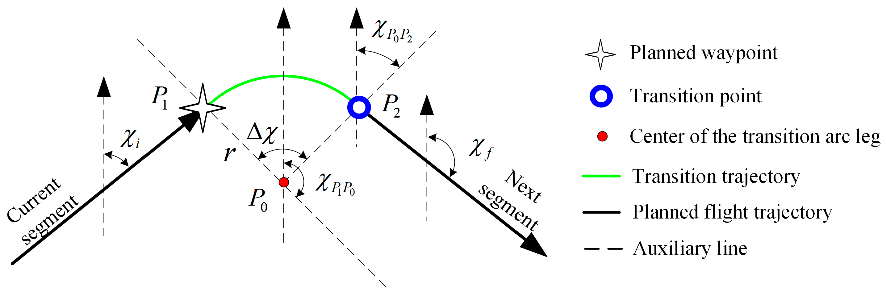
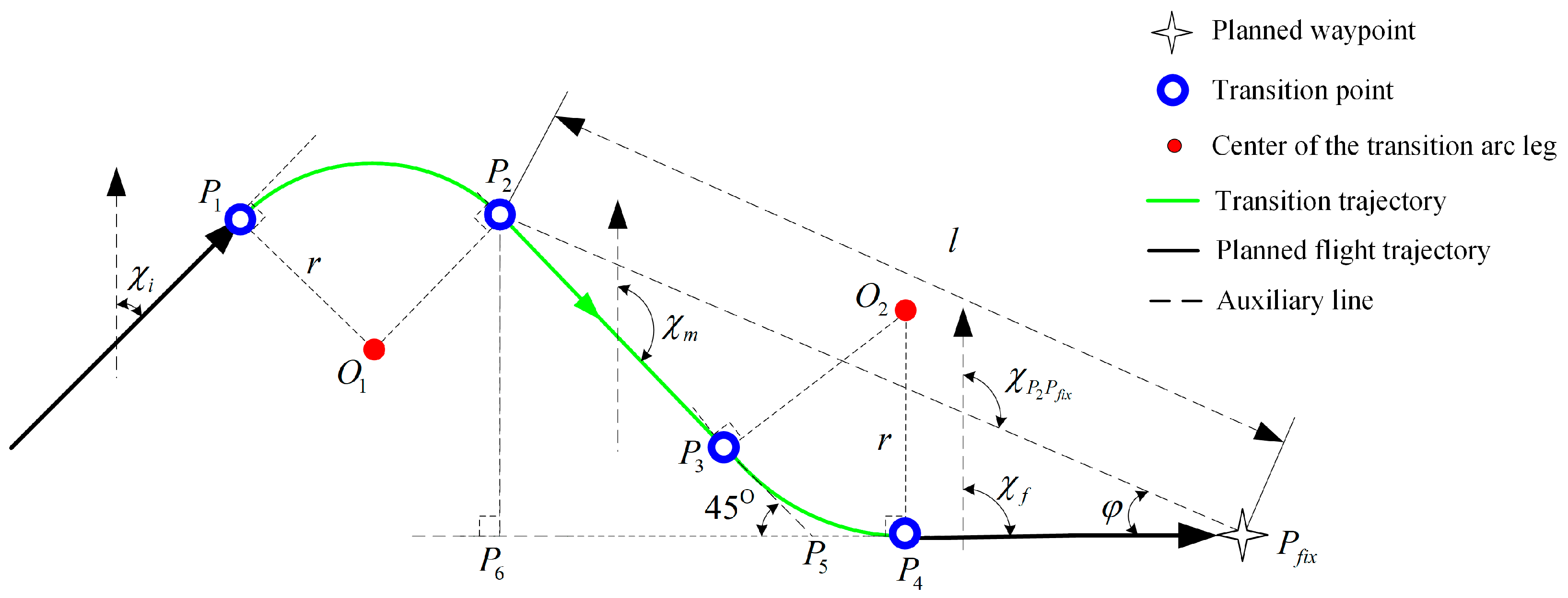
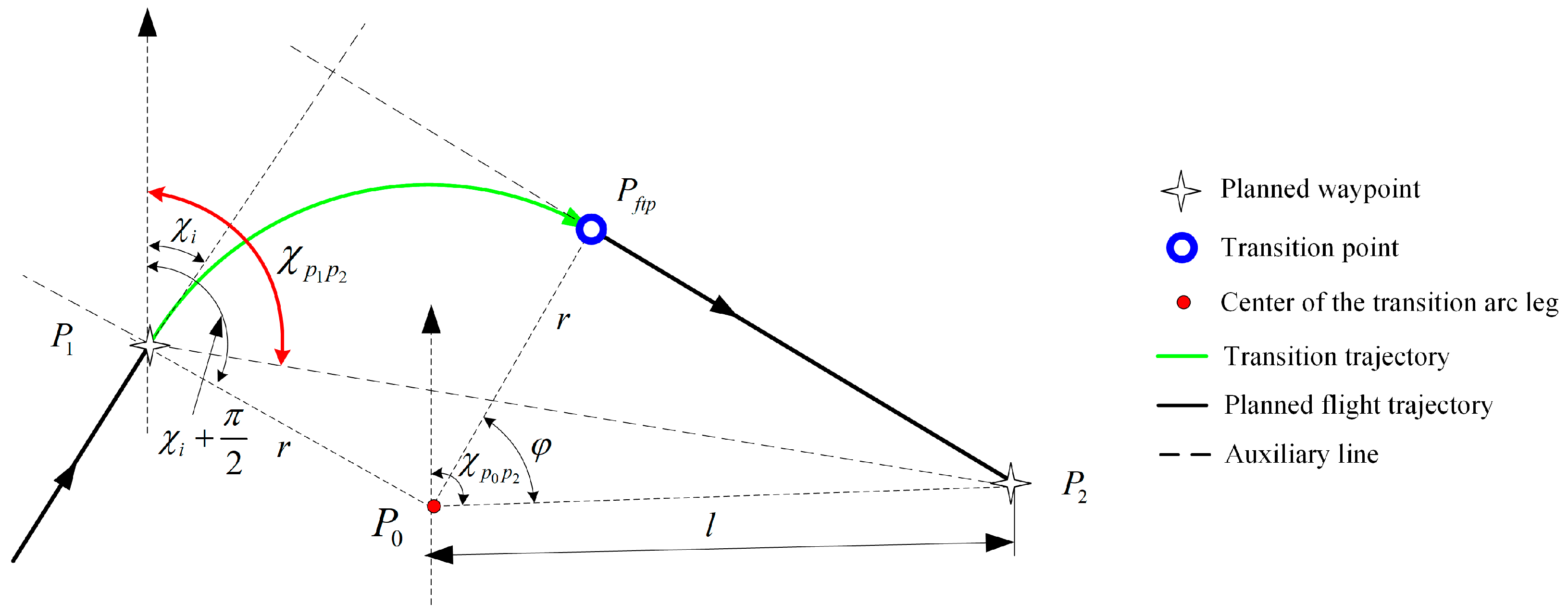
3. Generation of Lateral Navigation Transition Path

Since the RNP AR approach requires high guidance accuracy, the automatic flight system (AFS) guides the aircraft to track the planned route most of the time. Then, an important issue is generating the lateral navigation transition path, including constructing the lateral navigation transition path and determining the lateral segment switching strategy.

3.1. Construction of Lateral Navigation Transition Path

There are several lateral navigation transition paths in ARINC specification 424-21, which are tangent transition, position interception, 45° interception, direct transition, and arc interception. In order to realize automatic flight with high precision, it is necessary to generate the lateral navigation transition paths between different segments. Considering the application conditions of each lateral navigation transition path, the construction principle of each lateral navigation transition path is given as follows:

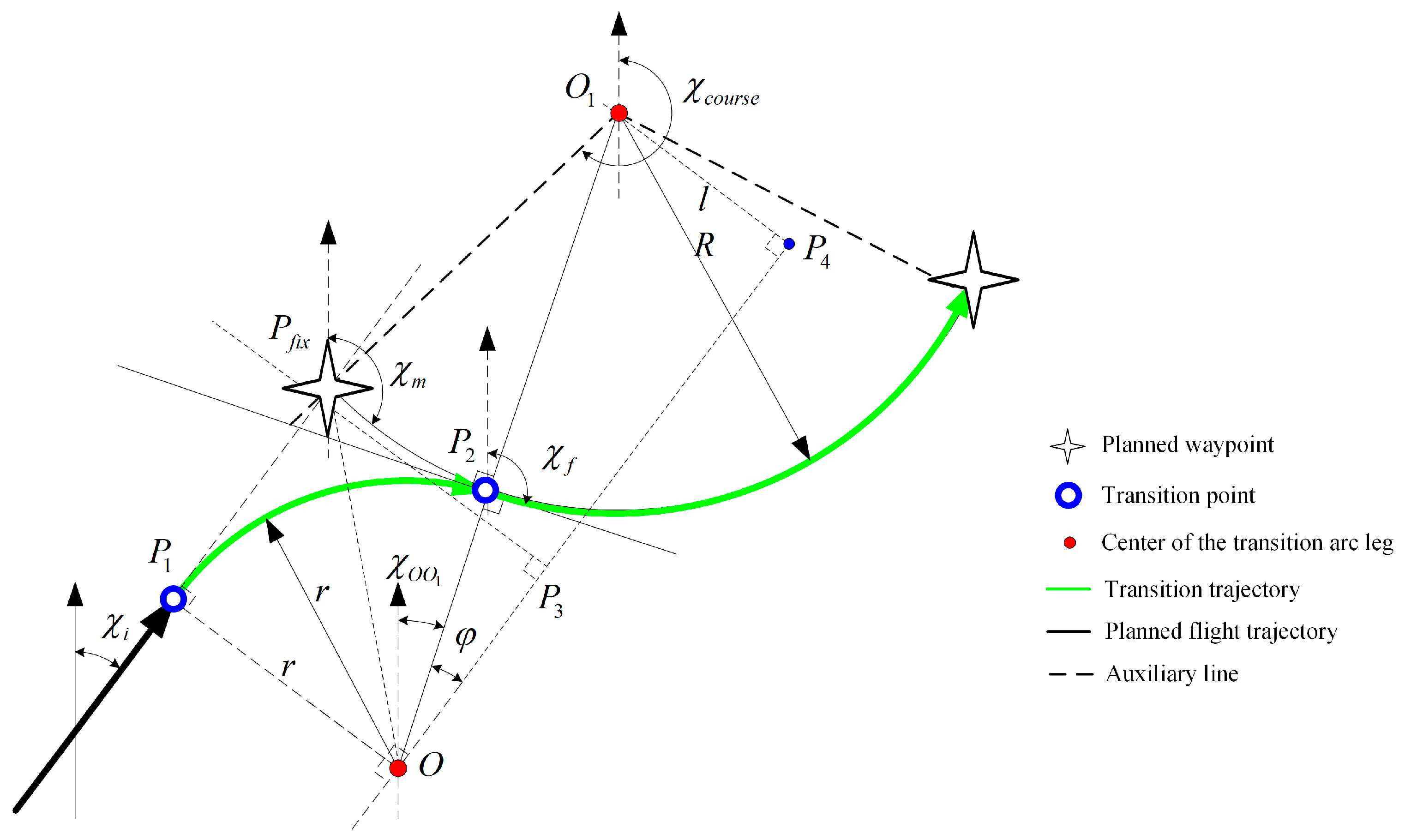
(1)

Tangent transition

If the azimuth angle of the current segment (${\chi }_i$) and the azimuth angle of the next segment (${\chi }_f$) are known, and there are no overflight requirements at the fixed point, tangent transition is applicable. Then, tangent transition is able to construct the lateral navigation transition path of the segment combination of the CF segment, TF segment, DF segment, and FA segment, such as DF-CF, DF-FA, TF-TF, and so on.

The tangent transition can be divided into two cases. In one case, the current segment and the next segment intersect at a fixed point, i.e., the ending point of the current segment is the starting point of the next segment, as shown in Figure 4. In the other case, both the current segment and the next segment are described with a fixed point and a known azimuth angle, but the intersection point is unknown, as shown in Figure 5.

In the first case, the known conditions include the coordinate of $P_{fix}$, the azimuth angle of the current segment (${\chi }_i$) and the azimuth angle of the next segment (${\chi }_f$). In the second case, the known conditions include the coordinate of $P_{fix1}$, the coordinate of $P_{fix2}$, the azimuth angle of the current segment (${\chi }_i$), and the azimuth angle of the next segment (${\chi }_f$). In both cases, the information to be solved contains the coordinate of the starting point of the transition path ($P_1$), the coordinate of the ending point of the transition path ($P_2$), and the coordinate of the circle center of the transition path ($P_0$).

(2)

Position interception

Position interception is applicable to the following situations: the coordinate of the ending point of the current segment is known and it is an overflight point, and the azimuth angle of the next segment is known.

The construction principle of position interception is shown in Figure 6. The known conditions include the coordinate of the ending point of the current segment ($P_1$), the azimuth angle of the current segment (${\chi }_i$), and the azimuth angle of the next segment (${\chi }_f$). The information to be solved contains the coordinate of the circle center of the transition path ($P_0$) and the coordinate of the ending point of the transition path ($P_2$).

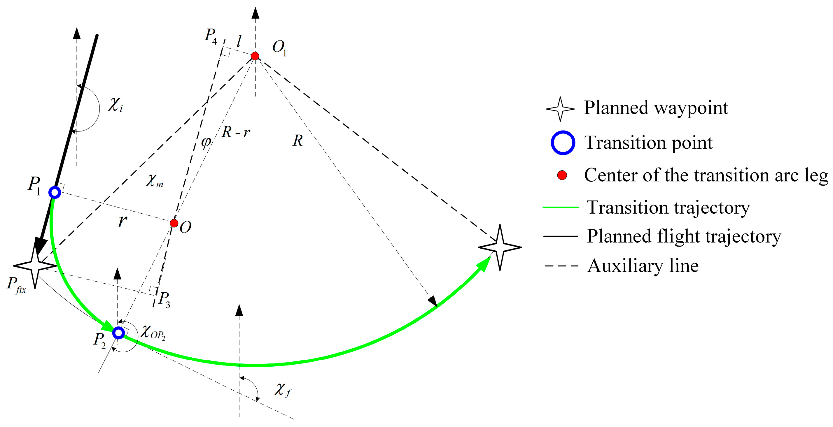
(3)

45° interception

If the coordinate of the ending point of the current segment and the azimuth angle of the current segment are known, and the space position of the next segment is also known, 45° interception is applicable.

The construction principle of 45° interception is shown in Figure 7, and it can be seen that 45° interception is essentially a combination of position interception and tangent transition. The known conditions include the coordinate of the ending point of the current segment ($P_1$), the azimuth angle of the current segment (${\chi }_i$), the coordinate of the fixed point on the next segment ($P_{fix}$), and the azimuth angle of the next segment (${\chi }_f$). The information to be solved contains the coordinate of $O_1$, $O_2$, $P_2$, $P_3$, and $P_4$.

(4)

Direct transition

Direct transition is applicable to the following situations: the coordinate of the ending point of the current segment and the azimuth angle of the current segment are known, and the coordinate of the fixed point on the next segment is known.

The construction principle of direct interception is shown in Figure 8. The known conditions include the coordinate of the ending point of the current segment ($P_1$), the azimuth angle of the current segment (${\chi }_i$), and the coordinate of the fixed point on the next segment ($P_2$). The information to be solved contains the coordinate of the circle center of the transition path ($P_0$) and the coordinate of the ending point of the transition path ($P_{ftp}$).

(5)

Arc interception

Arc interception is applicable when the next segment is an arc segment (AF segment or RF segment), and it can be divided into two cases, as shown in Figure 9 and Figure 10.

The key to arc interception is to construct an arc segment, which is tangent to the next segment. The known conditions include the coordinate of the circle center of the next arc segment ($O_1$), the radius of the next arc segment ($R$), the coordinate of the fixed point on the next arc segment ($P_{fix}$), the turn direction of the next arc segment, the current aircraft position, and the azimuth angle of the aircraft (${\chi }_i$). The information to be solved contains the coordinate of the starting point of the transition path ($P_1$), the coordinate of the ending point of the transition path ($P_2$), and the coordinate of the circle center of the transition path ($O$).

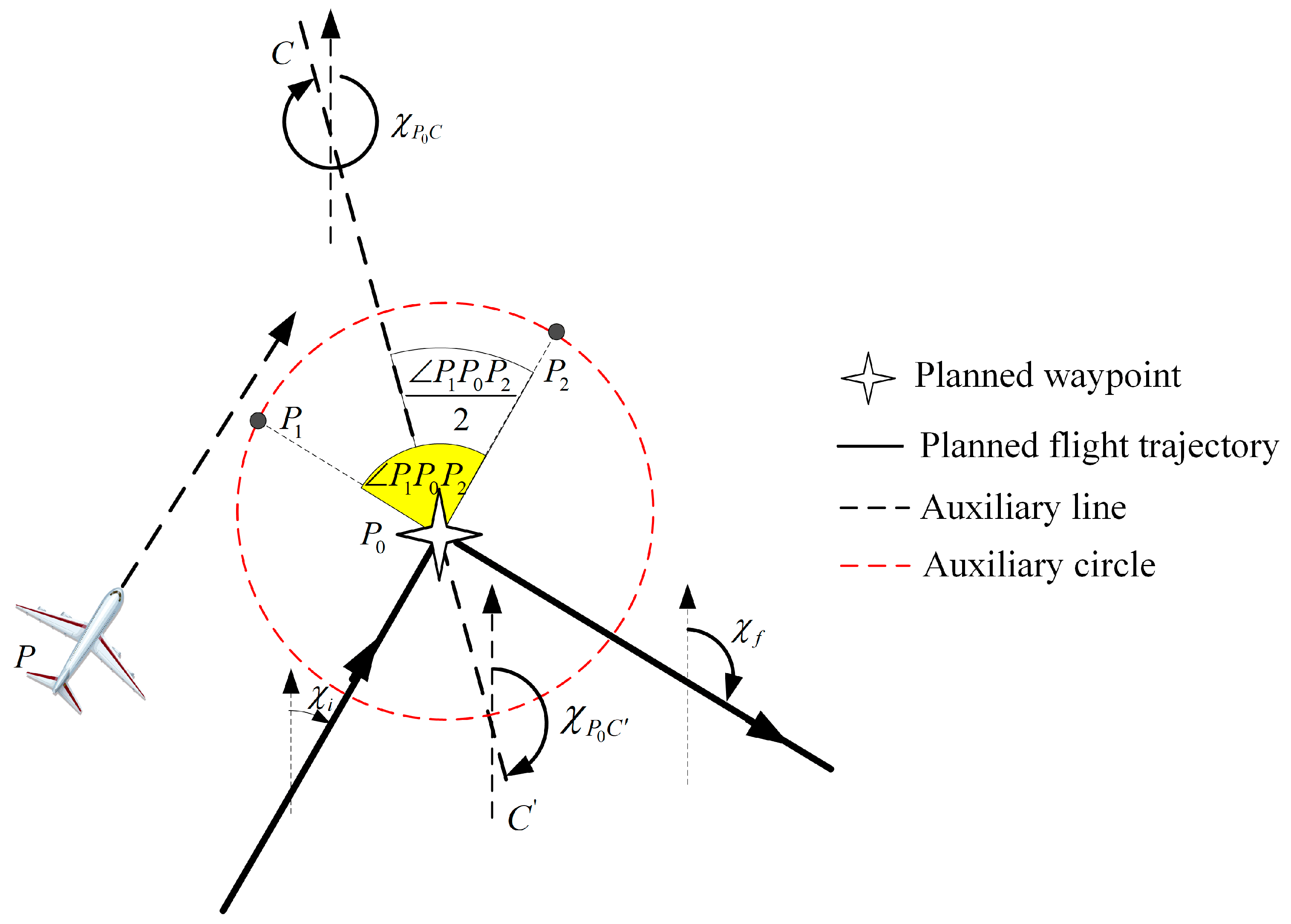
3.2. Lateral Segment Switching Strategy

Currently, the distance-based switching strategy is widely adopted, as shown in Figure 11. There is a preset threshold ($D_s$), if the distance between the current aircraft position and ending point of the current segment is less than $D_s$, then it will automatically switch to the next segment.

This method is simple in principle and easy to implement. Nevertheless, due to navigation system error, flight technical error, wind disturbance, and other factors, it is almost impossible for the aircraft to completely track the planned trajectory. When the deviation between the aircraft and the planned trajectory is large, the switching method based on the distance strategy is not applicable.

Therefore, a switching method based on the angular bisector is introduced in this paper, as shown in Figure 12.

In Figure 12, $P_0$ is the ending point of the current leg, ${\chi }_i$ is the azimuth angle of the current leg, and ${\chi }_f$ is the azimuth angle of the next leg. The switching method based on the angular bisector can be described as follows:

The turning direction can be judged according to the azimuth angle of the current leg and the azimuth angle of the next leg, and the process can be depicted as

If $0<{\chi }_i<\frac{\pi }{2}$, then

$$k_{turn}=\{\begin{array}{ll}1,& 0<{\chi }_f-{\chi }_i<\pi \\ -1,& \frac{-\pi }{2}<{\chi }_f-{\chi }_i<0\\ -1,& \pi <{\chi }_f-{\chi }_i<2\pi \end{array}$$

(24)

If $\frac{\pi }{2}<{\chi }_i<\pi$, then

$$k_{turn}=\{\begin{array}{ll}1,& 0<{\chi }_f-{\chi }_i<\pi \\ -1,& -\pi <{\chi }_f-{\chi }_i<0\\ -1,& \pi <{\chi }_f-{\chi }_i<\frac{3\pi }{2}\end{array}$$

(25)

If $\pi <{\chi }_i<\frac{3\pi }{2}$, then

$$k_{turn}=\{\begin{array}{ll}1,& -\frac{3\pi }{2}<{\chi }_f-{\chi }_i<-\pi \\ 1,& 0<{\chi }_f-{\chi }_i<\pi \\ -1,& -\pi <{\chi }_f-{\chi }_i<0\end{array}$$

(26)

If $\frac{3\pi }{3}<{\chi }_i<2\pi$, then

$$k_{turn}=\{\begin{array}{ll}1,& -2\pi <{\chi }_f-{\chi }_i<-\pi \\ 1,& 0<{\chi }_f-{\chi }_i<\frac{\pi }{2}\\ -1,& -\pi <{\chi }_f-{\chi }_i<0\end{array}$$

(27)

Taking $P_0$ as the center, draw an auxiliary circle with radius $R_{P0}$. The current leg intersects the auxiliary circle at $P_2$, and the next leg intersects the auxiliary circle at $P_1$. Then $\angle P_1{P}_0{P}_2$ can be calculated by

$$\angle P_1{P}_0{P}_2=\{\begin{array}{ll}\pi -\left|{\chi }_f-{\chi }_i\right|,& \left|{\chi }_f-{\chi }_i\right|<\pi \\ \left|{\chi }_f-{\chi }_i\right|-\pi ,& \left|{\chi }_f-{\chi }_i\right|>\pi \end{array}$$

(28)

It can be seen that $P_0$ is on the intersection line between the switching plane and the ground level from Figure 4. If the starting point of the intersection line is $P_0$, the azimuth angle of the intersection line can be ${\chi }_{P_{0}C}$ or ${\chi }_{P_0{C}^{\prime }}$, and ${\chi }_{P_{0}C}$ can be calculated by

If $0<{\chi }_i<\frac{\angle P_1{P}_0{P}_2}{2}$, then

$${\chi }_{P_{0}C}=\{\begin{array}{ll}{\chi }_i+\frac{\angle P_1{P}_0{P}_2}{2}& ,k_{turn}=-1\\ {\chi }_i-\frac{\angle P_1{P}_0{P}_2}{2}+2\pi ,& k_{turn}=1\end{array}$$

(29)

If $\frac{\angle P_1{P}_0{P}_2}{2}<{\chi }_i<\left(2\pi -\frac{\angle P_1{P}_0{P}_2}{2}\right)$, then

$${\chi }_{P_{0}C}=\{\begin{array}{ll}{\chi }_i+\frac{\angle P_1{P}_0{P}_2}{2},& k_{turn}=-1\\ {\chi }_i-\frac{\angle P_1{P}_0{P}_2}{2},& k_{turn}=1\end{array}$$

(30)

If $\left(2\pi -\frac{\angle P_1{P}_0{P}_2}{2}\right)<{\chi }_i<2\pi$, then

$${\chi }_{P_{0}C}=\{\begin{array}{ll}{\chi }_i+\frac{\angle P_1{P}_0{P}_2}{2}-2\pi ,& k_{turn}=-1\\ {\chi }_i-\frac{\angle P_1{P}_0{P}_2}{2},& k_{turn}=1\end{array}$$

(31)

Then, ${\chi }_{P_0{C}^{\prime }}$ can be calculated by

$${\chi }_{P_0{C}^{\prime }}=\{\begin{array}{ll}{\chi }_{P_{0}C}+\pi ,& {\chi }_{P_{0}C}<\pi \\ {\chi }_{P_{0}C}-\pi ,& {\chi }_{P_{0}C}>\pi \end{array}$$

(32)

As a result, the cross track distance ($\Delta D$) from the aircraft to the switching plane can be calculated using Equations (7) and (8). If $\Delta D_{last}\cdot \Delta D_{cur}<0$, then the lateral segment is supposed to be switched. $\Delta D_{last}$ is the cross track distance at the last time, and $\Delta D_{cur}$ is the cross track distance at current time.

3.3. Automatic Flight Guidance Strategy Supporting RNP AR Approach Procedure

The RNP AR approach requires high guidance accuracy, and the aircraft is guided by the automatic flight system in most cases. Based on the designed flight guidance law and the lateral segment switching strategy, the automatic flight guidance strategy supporting the RNP AR approach procedure is shown in Figure 13.

4. Simulation Verification

In order to demonstrate the effectiveness of the proposed guidance command generation method, a simulation example based on the RNP AR approach procedure of Jiuzhai Huanglong Airport is introduced.

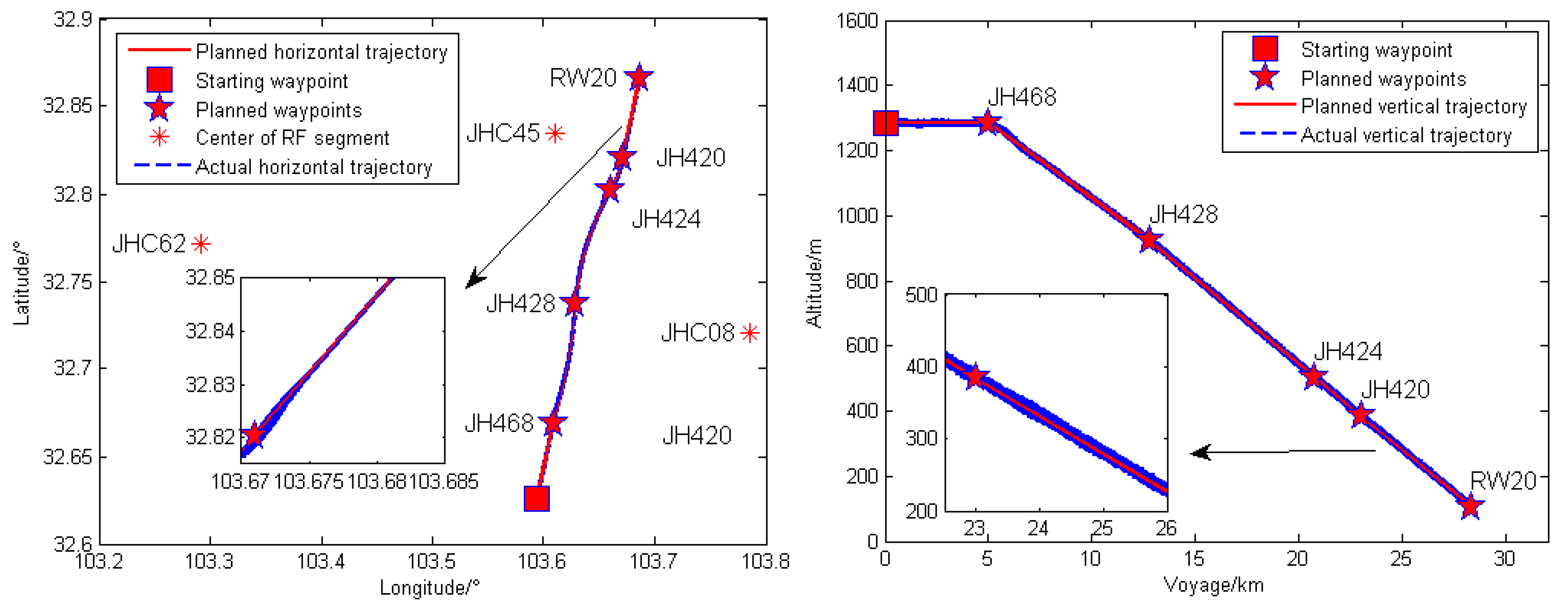
4.1. RNP AR Approach Procedure Flight Plan of Jiuzhai Huanglong Airport

The RNP AR approach procedure flight plan of Jiuzhai Huanglong Airport is shown in

Table 2. RNP AR approach procedure flight plan of Jiuzhai Huanglong Airport.

Waypoint Index	Starting Waypoint	JH468	JH428	JH424	JH420	RW20
Latitude/°	32.6261	32.6693	32.7370	32.8023	32.8022	32.8661
Longitude/°	103.5940	103.6087	103.6286	103.6603	103.6709	103.6865
Altitude/m	1284.73	1284.73	922.63	503.83	384.05	106.70
IAS/(m/s)	82.3	82.3	82.3	82.3	82.3	82.3
Leg type	IF	TF	RF	RF	RF	TF
Turn Direction	\	\	left	right	left	\
Center of RF segment	\	\	JHC62	JHC08	JHC45	\
Center latitude/°	\	\	32.7714	32.7207	32.8349	\
Center longitude/°	\	\	103.2921	103.7854	103.6101	\
Leg length/km	\	4.999	7.795	7.944	2.246	5.309
RNP/n mile	0.3	0.3	0.3	0.3	0.3	0.3

, and the planned horizontal trajectory and planned vertical trajectory based on the flight plan are shown in Figure 14.

4.2. Evaluation Indexes of the Guidance Effect

The requirements of the RNP AR approach for the flight guidance algorithm are mainly reflected in guidance accuracy, so flight technical error (FTE) is selected to evaluate the guidance effect of the proposed guidance algorithm.

FTE consists of lateral FTE and vertical FTE. The lateral FTE indicates the deviation between the aircraft position and the desired horizontal trajectory, and the vertical FTE indicates the deviation between the aircraft position and the desired vertical trajectory. The calculation method of lateral FTE ($FT{E}_{lat}$) and vertical FTE ($FT{E}_{vert}$) are given in [17].

Referring to «Minimum Aviation System Performance Standards: Required Navigation Performance for Area Navigation» (RTCA DO-236B) [18], for a specified segment with a given RNP value, the lateral FTE is supposed to meet Equation (33).

$$FT{E}_{lat}\le 0.4x$$

(33)

where $x$ represents the RNP value.

The requirements of vertical flight technical error when performing the RNP AR approach procedure is given in «Required Navigation Performance Authorization Required (RNP AR) Procedure Design Manual» (ICAO Doc 9905) [19], and the vertical FTE is supposed to meet Equation (34).

$$FT{E}_{vert}\le 75ft$$

(34)

Therefore, for the RNP AR approach procedure of Jiuzhai Huanglong Airport, the maximum lateral FTE is 222.24 m, and the maximum vertical FTE is 75ft, that is, 22.86 m.

4.3. Simulation Conditions

In order to evaluate the guidance effect of the proposed guidance algorithm, the Monte Carlo method is applied, and wind interference and sensor noise are considered.

The simulation conditions are described as follows:

(1)

The initial position of the aircraft is (32.6261°, 103.5940°), and the initial flight altitude is 1284.7 m.

(2)

The initial aircraft heading is 15.95°, and the initial indicated airspeed (IAS) is 82.3 m/s.

(3)

In the process of the RNP AR approach, the INS/GPS integrated navigation system is the main navigation source. In general, the error characteristics of GPS meet the first-order Markov process, and the positioning error model of GPS is shown as Equation (35).

$$\{\begin{array}{l}\delta \dot{\lambda }=-\frac{1}{{\tau }_{\lambda }}\delta \lambda +{\omega }_{\lambda }\\ \delta \dot{L}=-\frac{1}{{\tau }_L}\delta L+{\omega }_L\\ \delta \dot{h}=-\frac{1}{{\tau }_h}\delta h+{\omega }_h\end{array}$$

(35)

where $\delta \lambda$ is the longitude error, $\delta L$ is the latitude error, and $\delta h$ is the altitude error. ${\tau }_{\lambda }$, ${\tau }_L$, and ${\tau }_h$ are the correlation times. ${\omega }_{\lambda }$, ${\omega }_L$, and ${\omega }_h$ are driving white noise. These relative parameters are given in [20].

(4)

As for wind disturbance, referring to the precision approach requirements given in «Criteria for Approval of Category III Weather Minima for Takeoff, Landing, and Rollout» [21], the wind direction is subject to [0, 360°] uniform distribution variable, and the wind speed is subject to [0, 20 kt] uniform distribution variable.

(5)

The algorithm program is developed in the Windows 10 environment using MATLAB 2014a and Visual Studio 2013. In addition, the attribute of the processor is Intel(R) Core(TM) i5-9500 CPU @ 3.00 GHz, and the installed RAM is 16.00 GB.

4.4. Verification of Guidance Parameter Tuning Method

In order to determine the flight guidance law parameters, the guidance parameter tuning problem is considered an optimization problem and solved using the PSO algorithm as described in Section 2.3.

Take the CX segment as an example to illustrate the effectiveness of the flight guidance law parameter tuning strategy via PSO algorithm. The initial longitude of the aircraft is 108°, the initial latitude is 34.05°, and the initial heading is 90°. The fixed point of the CX segment is P (34°, 108°), and the azimuth angle of the CX segment is 90°.

The flight guidance law configuration of the CX segment is ${\varphi }_c=k_d\cdot \Delta D+k_{\chi }\cdot ({\chi }_{leg}-\chi )\cdot V_{GND}$. Based on the engineering experience and the aircraft model performance, it is known that $k_d\in \left(0,0.2\right)$ and $k_{\chi }\in -\left(0.1,0\right)$. We set the population size to 10, and the number of iterations is 10. The simulation results are shown as follows (Figure 15), and $k_{\chi }=-0.023$, $k_d=0.088$.

Adjusting the number of iterations to 100, the simulation results are shown as follows (Figure 16), and $k_{\chi }=-0.028$, $k_d=0.122$

It can be seen from the results that the flight guidance law parameter tuning strategy via PSO algorithm is effective, and only a small population size and iterations can achieve good results.

4.5. Verification of Guidance Command Generation Method

According to the simulation conditions set in Section 4.3, 500 Monte Carlo simulations are carried out based on the RNP AR approach procedure of Jiuzhai Huanglong Airport, and the maximum lateral FTE and maximum vertical FTE are counted to evaluate the guidance effect.

The flight trajectories are shown in Figure 17, and the maximum lateral FTE and maximum vertical FTE are shown in Figure 18.

The simulation results show that the proposed guidance algorithm can guide the aircraft to fly along the planned trajectory, and the maximum lateral FTE and the maximum vertical FTE can meet the guidance requirements of the RNP AR approach procedure of Jiuzhai Huanglong Airport.

After statistical analysis, it can be obtained that the mean of the maximum lateral FTE is 89.319 m, and the maximum value is 103.702 m. The mean of the maximum vertical FTE is 15.070 m, and the maximum value is 20.157 m. In addition, the standard deviation of the maximum lateral FTE is 1.246 m, and the standard deviation of the maximum vertical FTE is 1.120 m. These data show that the distribution of the actual trajectories is very concentrated and basically consistent with the planned trajectory.

As a result, it can be drawn that the proposed guidance algorithms can provide the lateral and vertical guidance capabilities that meet the requirements of the RNP AR approach.

5. Conclusions and Future Work

In this paper, a 3D precise guidance command generation method for civil aircraft to perform the RNP AR approach procedure is proposed, including lateral flight guidance law and vertical flight guidance law. Then, the construction principle of the lateral navigation transition paths between different segments are given, and a lateral segment switching method via the angular bisector is presented to achieve automatic flight. Finally, a simulation example based on the RNP AR approach procedure of Jiuzhai Huanglong Airport is introduced to illustrate the effectiveness of the proposed algorithm.

Although precise flight guidance is important during the process of the RNP AR approach at high-plateau airports, there also are some other significant problems need to be solved, such as the construction of high-precision and high-reliability navigation systems, low temperature correction of barometric height, etc. These are the problems that must be settled to ensure flight safety when implementing the RNP AR approach at high-plateau airports.

References

- Chen, N.; Sun, Y.; Wang, Z.; Peng, C. Improved LS-SVM Method for Flight Data Fitting of Civil Aircraft Flying at High Plateau. Electronics 2022, 11, 1558. [Google Scholar] [CrossRef]
- Shao, Q.; Yang, M.; Xu, C.; Wang, H.; Liu, H. Fire risk analysis of runway excursion accidents in high-plateau airport. IEEE Access 2020, 8, 204400–204416. [Google Scholar] [CrossRef]
- Zhang, P.; Yang, L.; Zang, Z. Design Flow and Flight Safety of RNP-AR Flight Procedure in Civil Aviation Airport. In Proceedings of the 2021 IEEE 3rd International Conference on Civil Aviation Safety and Information Technology (ICCASIT), Changsha, China, 20–22 October 2021. [Google Scholar]
- Unkelbach, R.M.; Dautermann, T. Development and evaluation of an RNP AR approach procedure under tight airspace constraints. CEAS Aeronaut. J. 2022, 13, 613–625. [Google Scholar] [CrossRef]
- Unkelbach, R. Development of an RNP AR APCH approach procedure within tight airspace constraints. Ph.D. Thesis, Technische Universität Berlin, Berlin, Germany, 2021. [Google Scholar]
- Savas, T.; Sahin, O. Safety assessment of RNP AR approach procedures. Int. J. Sustain. Aviat. 2017, 3, 29–42. [Google Scholar] [CrossRef]
- Salgueiro, S.; Hansman, R.J. Potential Safety Benefits of RNP Approach Procedures. In Proceedings of the 17th AIAA Aviation Technology, Integration, and Operations Conference, Denver, CO, USA, 5–9 June 2017. [Google Scholar]
- McDonald, J.; Kendrick, J. Benefits of tightly coupled GPS/IRS for RNP operations in terrain challenged airports. In Proceedings of the 2008 IEEE/ION Position, Location and Navigation Symposium, Monterey, CA, USA, 6–8 May 2008. [Google Scholar]
- Sahin, O.; Turgut, E.T.; Aslaner, S.; Usanmaz, O. Fuel and carbon dioxide emission assessment for a curved approach procedure. J. Aircr. 2019, 56, 2108–2117. [Google Scholar] [CrossRef]
- Marheim, J.A.; Hengebol, P.; Newman, M.J. Performance based navigation (PBN) as a noise abatement tool. In Proceedings of the INTER-NOISE and NOISE-CON Congress and Conference Proceedings, Chicago, IL, USA, 26–29 August 2018. [Google Scholar]
- Morscheck, F. Noise mitigation optimization of A-RNP/RNP AR approaches. In Proceedings of the 2018 Aviation Technology, Integration, and Operations Conference, Atlanta, GA, USA, 25–29 June 2018. [Google Scholar]
- Entzinger, J.O.; Nijenhuis, M.; Uemura, T. Assessment of human pilot mental workload in curved approaches. In Proceedings of the 2013 Asia-Pacific International Symposium on Aerospace Technology (APISAT), Takamatsu, Japan, 20–22 November 2013. [Google Scholar]
- Gouldey, D. Determining operational benefits of required navigation performance (RNP) authorization required (AR) approaches. In Proceedings of the 2014 Integrated Communications, Navigation and Surveillance Conference (ICNS) Conference Proceedings, Herndon, VA, USA, 8–10 April 2014. [Google Scholar]
- Amai, O.; Matsuoka, T. Air traffic control real-time simulation experiment regarding the mixed operation between RNP AR and ILS approach procedures. In Proceedings of the 2015 International Association of Institutes of Navigation World Congress (IAIN), Prague, Czech Republic, 20–23 October 2015. [Google Scholar]
- Dautermann, T.; Ludwig, T.; Altenscheidt, L.; Geister, R.; Blase, T. Automatic speed profiling and automatic landings during advanced RNP to xLS flight tests. In Proceedings of the 2017 IEEE/AIAA 36th Digital Avionics Systems Conference (DASC), St. Petersburg, FL, USA, 17–21 September 2017. [Google Scholar]
- ARINC424-21; Navigation System Database ARINC SPECIFICATION 424-21. AEEC: Reston, VA, USA, 2016.
- Zhai, S.; Li, G.; Jia, Q.; Li, Z.; Cai, W. Design of Guidance Law for Automatic Landing Meeting the CAT III Standard. In Proceedings of the Asia-Pacific International Symposium on Aerospace Technology (APISAT), Jeju, Korea, 15–17 November 2021. [Google Scholar]
- RTCA DO-236B; RTCA DO-236B Minimum Aviation System Performance Standards: Required Navigation Performance for Area Navigation. Radio Technical Commission for Aeronautics: Washington, DC, USA, 2003.
- International Civil Aviation Organization. Doc 9905 Required Navigation Performance Authorization Required (RNP AR) Procedure Design Manual; International Civil Aviation Organization: Montreal, QC, Canada, 2009. [Google Scholar]
- Qin, Y.; Zhang, H.; Wang, H. Kalman Filter and Integrated Navigation Theory, 3rd ed.; Northwestern Polytechnical University Press: Xi’an, China, 2015; pp. 292–294. [Google Scholar]
- AC 120-28D; AC 120-28D Criteria for Approval of Category III Weather Minima for Takeoff, Landing, and Rollout. Federal Aviation Administration: Washington, DC, USA, 1999.