1. Introduction
The growing interest in deep space exploration, for which the NASA Artemis Program [
1], and recent commercial moon ventures [
2], are clear examples, has led to the need for new technologies to overcome the challenges of upcoming space missions. To ensure the long-term viability of these activities, effective mission and trajectory designs, including proximity operations, are of vital importance, such as, for example, regular resupply and crew transportation missions to support the establishment of newly crewed outposts in cislunar space, such as the Lunar Gateway [
3]. Therefore, new trajectory design, guidance, and navigation capabilities have been identified as key enabling technologies to support the expansion of human space activity beyond Earth’s orbit, as highlighted by the Global Exploration Roadmap of the International Space Exploration Coordination Group [
4,
5].
While near-Earth missions may be completely analyzed under a perturbed Keplerian paradigm, deep space missions require a different modeling approach, in which multi-body gravitational interactions play a major role. Along this line, early mission design is usually accomplished through the use of the Circular Restricted Three-Body Problem (CR3BP) as the main modeling strategy, due to its ability to retain major dynamical transport structures while still being relatively simple.
Great effort has been dedicated to the analytical and numerical determination of dynamical structures in the CR3BP. Advancing on the seminal work of Poincaré [
6], practical CR3BP orbit solutions were found, based on a Hamiltonian analysis of the dynamics around the collinear libration points, as studied by Richardson [
7] and, numerically, by Howell and Pernicka [
8]. In this sense, Dynamical Systems Theory has always been insightful in revealing the manifold-driven transport phenomena in the CR3BP, and has, eventually, become the standard analysis tool nowadays. Its application to multi-body mission design may be traced back to the seminal work of the Barcelona Group and Koon et al. [
9,
10].
Libration Point Orbits (LPOs), a natural solution of the CR3BP, have been identified as ideal locations for deep space exploration-related activities, including the establishment of the Lunar Gateway space station. While the triangular libration points also exhibit such solutions, these are usually found less practical for space mission design purposes and, thus, this work considers only (unless otherwise specified) LPOs associated to the collinear libration points. These include periodic and quasi-periodic orbital families, which exhibit highly interesting features, due to their ability to maintain continuous communication with the Earth or to avoid solar eclipses. However, their intrinsic orbital instability yields relatively short time scales for divergence if the spacecraft abandons the nominal LPO, or when perturbational acceleration sources, such as third body perturbations or solar radiation pressure, are introduced into the analysis. As a result, tremendous effort has been devoted over the last three decades to the problem of trajectory control and stationkeeping of LPO, initiated by the pioneering work of Farquhar [
11,
12]. In the development of such control strategies, Dynamical Systems Theory has proven an invaluable and insightful theoretical tool, on which most different control policies have been built. Early stationkeeping design attempts exploited the periodic nature of these orbits, allowing for an approach based on Floquet’s theory, which led to the `Floquet Mode’ stationkeeping strategy, first proposed by Wiesel and Shelton [
13] and Simo et al. [
14], and later applied to the stationkeeping of translunar LPOs [
15]. New stationkeeping policies have since followed. Hou et al. [
16] proposed impulsive control strategies similar to the Floquet approach, which allowed its applicability to extend to the real Earth–Moon system by relying on quasi-periodic orbits referred to as dynamical substitutes. Héritier and Howell [
17] looked into harnessing natural, multi-body dynamics to minimize the drift of unstable relative dynamics. Muralidharan et al., through a series of works [
18,
19,
20], leveraged Cauchy–Green Tensor policies to solve the stationkeeping problem.
The aforementioned works proposed effective control strategies that relied heavily on Dynamical Systems Theory and exploited the properties of intrinsic structures of the CR3BP, resulting in impulsive strategies. However, they overlooked the plethora of techniques readily available in both classical and modern control theories, in which quadratic regulation is among the most relevant and widely explored techniques. Along this line, Breakwell et al. [
21] were among the first to approach the LPO trajectory control problem from a classical control viewpoint, by proposing a linear quadratic regulator for stationkeeping of a translunar halo orbit. Gurfil and Kasdin proposed a time-varying, continuous, linear quadratic control law, along with an internal disturbance model, that rendered a robust disturbance rejection performance [
22], and they also investigated the early use of neural networks for tracking control and disturbance rejection in this context [
23]. Marchand and Howell also developed continuous control strategies of increasing complexity based on linear and non-linear quadratic regulators and input/output feedback linearization [
24], as well as through numerical solutions to the optimal control problem [
25]. Nazari et al. [
26] proposed three control strategies combining continuous LQR control and Floquet theory using periodic control gains, which relied, respectively, on a time-periodic infinite horizon LQR, a backstepping technique with time-invariant LQR, and a dead-band periodic-gain controller. Lian et al. [
27] investigated the use of discrete-time sliding mode control and a discrete time linear quadratic regulator for stationkeeping of the real Earth–Moon LPO (i.e., with a complete Solar System model under a real ephemerides model), resulting in discrete control suitable for impulsive manoeuvres. Using a simple linear extended state observer, Narula and Biggs [
28] extended an LQR control scheme to enable continued tracking in the event of thruster failure and the presence of disturbances and they also demonstrated that, in combination with a sliding mode or an adaptive control, asymptotic tracking could be achieved. Qi and de Ruiter [
29] extended the use of backstepping controllers for stationkeeping of LPOs under practical navigational and executional constraints, a real ephemerides model and solar radiation pressure.
Shirobokov et al. presented a thorough, extensive survey on LPO stationkeeping strategies [
30], although they did not (understandably) compile the continued developments which followed in recent years in these lines. Current ongoing research includes that of Elliott and Bosanac [
31,
32], who are looking into LPO stationkeeping controllers based on an alternative set of geometric coordinates, and Gao et al. [
33,
34,
35,
36], who are investigating high-order dynamical systems for low-thrust stationkeeping of LPOs. Li and Hou have recently developed novel stationkeeping approaches to the control of triangular point orbits [
37]. Modern control schemes, such as Model Predictive Control, have also been recently applied to the LPO stationkeeping problem [
38,
39]. Interestingly, Bonasera, Bosanac, LaFarge et al. [
40,
41,
42,
43], are looking into reinforcement learning approaches to the LPO stationkeeping problem.
Relevant to our study, Hamiltonian mechanics have also been successfully applied to the problem of stationkeeping, leading to noteworthy control policies. Scheeres and Vinh [
44] developed a feedback control law based on the local eigenstructure of the LPO, which allowed for oscillatory motions in the center manifold. Jung and Kim [
45] proposed a switching Hamiltonian structure-preserving control and, more recently, Carletta et al. exploited Hamiltonian formalism [
46,
47] to develop a linear feedback compact stationkeeping law in the Sun-Mars elliptic restricted three-body problem LPOs, advancing the field to more complicated multi-body contexts. Along this line, Xu, Liang and Fu [
48] proposed a Hamiltonian structure-preserving control for LPO, which they successfully extended to the bi-circular four-body problem (i.e., time-periodic dynamics), and later to time-dependent dynamics, such as the relative orbital motion along low-energy transfer trajectories in the CR3BP [
49], which is a path also investigated by Cheng et al. [
50].
Despite all these publications focusing on trajectory control around LPOs, it is worth noting that a few publications have also looked into the general problem of relative co-orbital motion in the CR3BP, which is the focus of this work. It was not until recently that the multi-body relative motion problem attracted the Astrodynamics and Control communities’ attention. Thus, the development of control strategies that stem from a relative dynamics approach, and which exploit the natural solutions of the latter, remains yet to be fully explored. Richardson first presented a particular CR3BP relative motion model under the premise of the motion bounded to the collinear equilibrium points [
7]. Luquette [
51] and Franzini [
52] were among the first to present relative motion models and linearizations not necessarily bounded to the vicinity of these points in the CR3BP. Another interesting contribution is the work by Colagrossi et al. [
53], who have long studied rendezvous and repositioning algorithms in non-Keplerian orbits, analyzing relative dynamics using Floquet modes, among other approaches [
53,
54,
55]. Elliott and Bosanac looked into the relative motion problem through local toroidal coordinates [
31,
32,
56]. Lizy-Destrez et al. [
57] presented methods and results related to strategies for far and close rendezvous, and compared different linear and nonlinear models for cislunar relative motion. More recently, in a series of works, Zuehlke et al. studied natural relative motion solutions in the Restricted Three-Body Problem [
58,
59,
60].
It is worth again emphasizing the relevant role of Dynamical Systems Theory and Hamiltonian Mechanics in the study of the CR3BP, rooted at the core of most of the reviewed continuous-thrust LPO stationkeeping policies. It is precisely this rationale that motivated the present work. In particular, the aim of this investigation was two-fold. First, a Hamiltonian formulation of the relative co-orbital problem in the CR3BP is presented, upon which novel approaches to the linearization of the relative motion are introduced. Connections between the absolute and relative co-orbital dynamics are also established, based on the reduced normal form of the Hamiltonian, and natural transport structures in the relative case are explored. Based on this analytical formulation, and the analogies between absolute and relative dynamics and their associated structures, an optimal reduced-order, continuous stationkeeping controller is derived, hybridizing energy-shaping control and classical unstable manifold regulation in relative Floquet coordinates. Compared to classical control techniques, the proposed controller is shown to provide better error performance at lower control expenses.
The remainder of this manuscript is organized as follows. In
Section 2, both the absolute and relative dynamics in the CR3BP are briefly revisited, and the aforementioned Hamiltonian formulation of the relative problem is then introduced. Both linear and nonlinear co-orbital dynamical models are analytically derived, and intrinsic relative solutions and associated transport phenomena are studied. Connections between the classical collinear dynamics and the relative problem are also established in virtue of the rendezvous Hamiltonian linearized normal form.
Section 3 profits from the previous results obtained and exploits Floquet Theory in the design of a hybrid SDRE–Koopman stationkeeping controller in the co-orbital phase space. The performance of the proposed regulator is demonstrated in a Monte-Carlo campaign, and comparison against previous literature techniques is also addressed. Finally,
Section 4 summarizes the main conclusions of this work and outlines open lines of research.
2. Relative Dynamics in the CR3BP and Hamiltonian Structure
This section develops the absolute LPO and relative co-orbital dynamics of motion within the CR3BP. In particular, a Hamiltonian derivation of the problem is introduced, along with an analysis of its associated solutions. Based on such formalism, connections between the two problems are presented and discussed.
It is worth noting that, here, the term “absolute” may perhaps be confusing, since the equations of motion for a spacecraft in an LPO are often stated relative to the synodic frame. Nonetheless, we feel that the word “absolute” is the natural counterpart for “relative”, and, therefore, for the sake of convenience, we hereafter refer to the motion of a single spacecraft in an LPO as an “absolute” motion, thereby saving the use of the term “relative” to refer strictly to the relative co-orbital motion between two spacecraft, namely a target and a chaser spacecraft.
2.1. Absolute Dynamics in the CR3BP
The governing equations of motion considered in this study are framed within the Circular Restricted Three-Body Problem (CR3BP). In the CR3BP, two celestial bodies of masses
are considered, known as
primaries, which revolve around their common center of mass under their mutual gravitational attraction describing Keplerian circular orbits. Third and fourth bodies, i.e.,
spacecraft, labelled
respectively, are considered with comparatively negligible masses
, such that their motions are driven by gravitational interaction with the primaries, and the primaries are not affected by the presence of the spacecraft. The motion of the spacecraft is conveniently studied in a co-rotating, synodic frame
, defined as follows: the
axis points from
to
, following the latter in its relative circular motion around
; the
axis is set perpendicular to the orbital plane of the primaries (along the angular momentum of the system); and the
axis completes a dextral frame. The origin of
is located at the barycenter of the system. When realised in the synodic frame, the primaries’ position vectors occupy fixed positions along the
axis. The unit vectors
are defined, respectively, along each of the coordinate axes of the synodic frame. This is illustrated in
Figure 1, which depicts the definition of the synodic frame with respect to the inertial frame
. The latter is arbitrarily defined to be aligned with
at the reference epoch
.
In the following, dimensionless coordinates are used, where the distance between the primaries is used as the characteristic length, the orbital period of the primaries around their common barycenter is taken as the characteristic time, and the masses of the primaries are referred to as the total mass of the system. In these dimensionless coordinates, the primaries revolve at one radian per unit of dimensionless time, and the reduced mass of
can be defined as
and the primaries are set at a unit length apart from each other, so their position vectors, constant when realised in the synodic frame, can be written as
Under the aforementioned setup, the motion of the spacecraft is governed by the following second-order ordinary differential equation
where
is the dimensionless spacecraft position vector, as measured by an observer in the synodic frame, and the overhead dot (˙) indicates derivatives with respect to the non-dimensional time. Tne vector
denotes the dimensionless angular velocity vector of the synodic frame
with respect to the inertial frame
. Again, note that, in non-dimensional units,
.
2.2. Relative Co-Orbital Dynamics in the CR3BP
The relative motion between two spacecraft, termed
target and
chaser, following the usual nomenclature, and now considered. We, here, recovered the treatment of the problem given in [
38]. In short, both vehicles are modeled as point masses, and the mutual gravity interaction is neglected. The target spacecraft is assumed to be cooperative and passive (i.e., with no orbital maneuvering capabilities), and its trajectory to be accurately known.
Let vectors
and
denote the positions of the target and chaser spacecraft, respectively, so their relative position vector is defined as
. Differentiating twice, with respect to time, and including the appropriate inertial terms, the following governing equations are obtained:
where
are the synodic frame coordinates of the relative position vector
,
are the synodic frame coordinates of the target spacecraft position vector
, and the control acceleration
is introduced for future concerns. A well-behaved numerical approach to the integration of Equation (
3) may be found in
Appendix A. The relative motion model is closed, assuming the target spacecraft ephemerides are known. Interestingly, Equation (
3) can be compactly written into a first-order, control-affine nonlinear system
where
is the state vector accounting for the Cartesian relative position and velocity of the chaser with respect to the target.
The State Transition Matrix (STM),
, can also be computed from the variational equations stemming from Equation (
3). Both the flow’s stability and stroboscopic map are available from the propagation of the STM of the system along a reference trajectory, which satisfies the first-order variational equations
where
J is the Jacobian of the general dynamics vector field
and
I is the identity matrix. For Linear Time-Invariant (LTI) dynamical systems,
, the STM is explicitly given by
where the operator
denotes a matrix exponential. Given the Hamiltonian nature of Equation (
3) (demonstrated in the following Sections), the STM can be shown to be symplectic, its determinant being 1 and its eigenvalues appearing in reciprocal pairs on the complex unit circle [
10]. The STM plays a fundamental role in determining the dynamical transport phenomena of the problem and is highly exploited hereafter.
2.3. Hamiltonian Formulation of the Relative Dynamics
Following the success of the Lagrangian and Hamiltonian formulations of the CR3BP LPO absolute dynamics [
9,
10], an analogous development is accomplished for the co-orbital case, in order to explore qualitatively the phase space structure and solutions to our advantage in the design of guidance schemes. Although the classical relative motion literature, such as [
51,
52], introduced different dynamic models in the CR3BP, none of them studied the problem from an analytical point of view. A Hamiltonian approach may result in insightful and useful results for Mission Design and Flight Dynamics purposes.
In virtue of the Euler–Lagrange equations, the acceleration terms in Equation (
3) may be obtained from the following total derivative of the total kinetic energy
T with respect to the relative position coordinates and time, including the inertial contributions of the rotating frame in which the orbital state is measured.
The relative dynamics Lagrangian function is completed by the potential function
, describing the gravitational interaction of the relative state with the primaries and the target. Recovering Equation (
3) again,
where
is the unit vector spanning the
axis of the position configuration space and
corresponds to each of the primaries’ gravitational parameters. Solving this gradient equation for
yields
Therefore, the Lagrangian function
, from which the relative dynamics may be derived, is finally given by
The application of the Euler–Lagrange equations to the functional
results in the dynamics described by Equation (
3), where the relative position vector
is identified as the generalized position coordinates and
as the associated generalized velocities.
Defining the conjugate momenta
as
the associated relative dynamics Hamiltonian is readily available from the Legendre transform of the Lagrangian
, namely,
The relative dynamics are then recovered from , using Hamilton’s canonical equations.
For numerical purposes, and to ease the derivation of reduced-order models, the potential function
may be expressed in a convergent Legendre series [
61,
62]
where the argument
is defined as the projection of the relative particle position
along the vector pointing from the target spacecraft to each of the primaries,
, (see
Figure 1), namely,
This result allows expressing of the Lagrangian and Hamiltonian functionals
as
The latter Hamiltonian function describes the relative state of a chaser with respect to a target spacecraft, expressed in the relative phase space, while being affected by two third-body gravitational perturbations, located at
[
61]. The associated gravitational potential to such fictitious primaries is not constant in time, but dictated by the instantaneous position of the target spacecraft, which follows a known time law
(achievable, in general, by the numerical integration of Equation (
2)). More specifically, the tangent bundle of the problem
is identified with the standard Euclidean tangent bundle, except for the collisions with the primaries,
.
A similar, yet less general, derivation of this Hamiltonian was presented by Richardson [
7] in his description of the motion of a particle around a libration point, which founded all classical studies on transport phenomena in the absolute CR3BP [
9,
10]. Richardson’s work can, indeed, be seen as the particularization of the relative Hamiltonian (
7) here proposed, for a steady target spacecraft fixed at a libration point. In this regards, our derivation generalizes that of Richardson to the case of a moving target spacecraft. Therefore, classical libration point dynamics is understood as the trivial instance of the relative CR3BP problem, where the target spacecraft is located at any of these equilibrium points. Following this rationale, the above Lagrangian and Hamiltonian functionals can be expressed as [
7]
where the relative Legendre coefficients
read
The target motion acts as a local time-dependent affine smooth transformation on the original primaries location
. This has profound effects on the expected dynamics. Using Hamilton’s canonical equations, it is clear that
The immediate consequence of the Hamiltonian dependence on time is the lack of the usual Three-Body problem energy integral, the Jacobi Constant. However, the existence of periodic relative orbits, to be demonstrated later, ensures the dynamics are not always necessarily dissipative [
63]. Still, the equations of motion do admit an energy-like integral given by
where
is the squared magnitude of the synodic velocity of the relative particle and
is the classical pseudo-potential function [
8]
As given by the above result, the target spacecraft, in its local transformation of the co-orbital phase space, introduces and sinks energy. Therefore, another consequence of this non-autonomous nature of the problem is that the analyses provided through traditional CR3BP invariant sets of the problem, such as a zero-velocity surfaces , are much more complex or even unavailable.
The relative motion problem can be autonomized through augmenting the state vector by
n, to include the target state evolution, hence, rising the dimensionality of the problem to
. However, and of particular relevance for this work, if the target is found to be located on an absolute (quasi)periodic orbit, such as any LPO, an orbit function
exists under whose effect the target’s flow is analytical and the autonomous problem dimension is
. Since the
T-periodic orbit is diffeomorphic to the circle
, the time variable can be replaced with an angle-like parameter
with periodic boundary conditions and linear flow
. The existence of a function such as
leads to the geometrical law
[
64,
65]. The exploitation of this geometrical law for integration purposes remains a current, open line of research.
2.4. Linearized and N-th Order Models
In the following, several linearized relative orbital motion models are derived, which are found especially interesting for the development of general GNC algorithms. Retaining first-order terms in
in Equation (
3) yields the Rendezvous Linear Model (RLM) [
51,
58,
66,
67], a standard for deep space GNC purposes nowadays, which can be compactly expressed in matrix form as
where
and
denotes 3-dimensional null and identity matrices, respectively. The Coriolis acceleration term
reads
and the Hessian matrix
can be computed as
where the operator ⊗ denotes the dyadic product,
are here unit vectors pointing from the
i-th primary to the target spacecraft
and
are coefficients defined as
Again, note that the RLM is still time-dependent, since the matrix depends on the target spacecraft’s location . Consequently, stability analysis of the model cannot be easily assessed, as the eigenspace and fixed points of the system depend explicitly on the target spacecraft’s motion.
The RLM is used to validate the analytical derivation of the relative CR3BP problem just presented. Given the (Hamiltonian) Lagrangian functional
in Equation (
6),
N-th order relative dynamics model may be derived by the application of Euler–Lagrange equations, reading
It is straightforward to derive the RLM model from the second-order expansion of the potential function,
,
With respect to the relative position vector, the derivation yields
Applying the Euler–Lagrange equations, and retaining up to first-order terms in , results in the RLM presented in the literature, thus completing the validity of the analytical model given in this work.
In specific cases, the linearized RLM can be further simplified, as for a target spacecraft fixed at a libration point, or on a periodic orbit around it. In such situations,
becomes constant or (quasi-)periodic, respectively. These latter cases define the Relative Libration Linear Models (RLLMs), which may be useful in the design of linear time-periodic, or time-invariant, control schemes [
38,
53,
54,
65,
68,
69,
70]. In such cases,
is given by
Therefore, under this assumption, the fundamental frequency
is reduced to the first order of the classical Richardson’s result
for the collinear points, as defined in [
7]. The relative dynamics are, therefore, uncoupled from the exact chaser’s and target’s trajectories while inheriting the LPO dynamics phase space solution structures [
65]. This latter model can be derived by the following process: (1) linearizing first the target and chaser spacecraft absolute motions around the collinear libration point of interest, and using Richardson’s model [
7,
8] to obtain the relative dynamics by direct subtraction
; (2) assuming the target motion occurs near the libration point, in the form of
, where
defines the location of the libration point in the synodic
x axis, and
is assumed to be at least quasi-periodic and of order
.
2.5. Higher-Order Models
As already introduced, the expansion of the relative motion Hamiltonian/Lagrangian in Legendre series allows derivqtion of motion models up to
N-th order, as in Equation (
11). This Section introduces second- and third-order models of the co-orbital dynamics by retaining up to the third-order terms in the expansion.
For the second-order case, the potential function is given by
Defining
, the second-order acceleration model, therefore, results in
where the first two terms of the right hand side are just the linear contribution of the RLM model. Retaining only second-order terms yields
where
is the Hessian matrix of the second-order expansion of the potential,
.
In the same way, for the third-order model, the expanded potential reads
giving rise to the following dynamics
The third-order model is, therefore, finally
Each order term in the expansion has a clear interpretation, comprising two different terms which quantify the projection of the gravity interaction of the chaser spacecraft with the two primaries in the relative phase space. The first term projects the gravitational acceleration along the relative position vector, , and the second one spans the associated orthogonal complementary projection through the linear operator, .
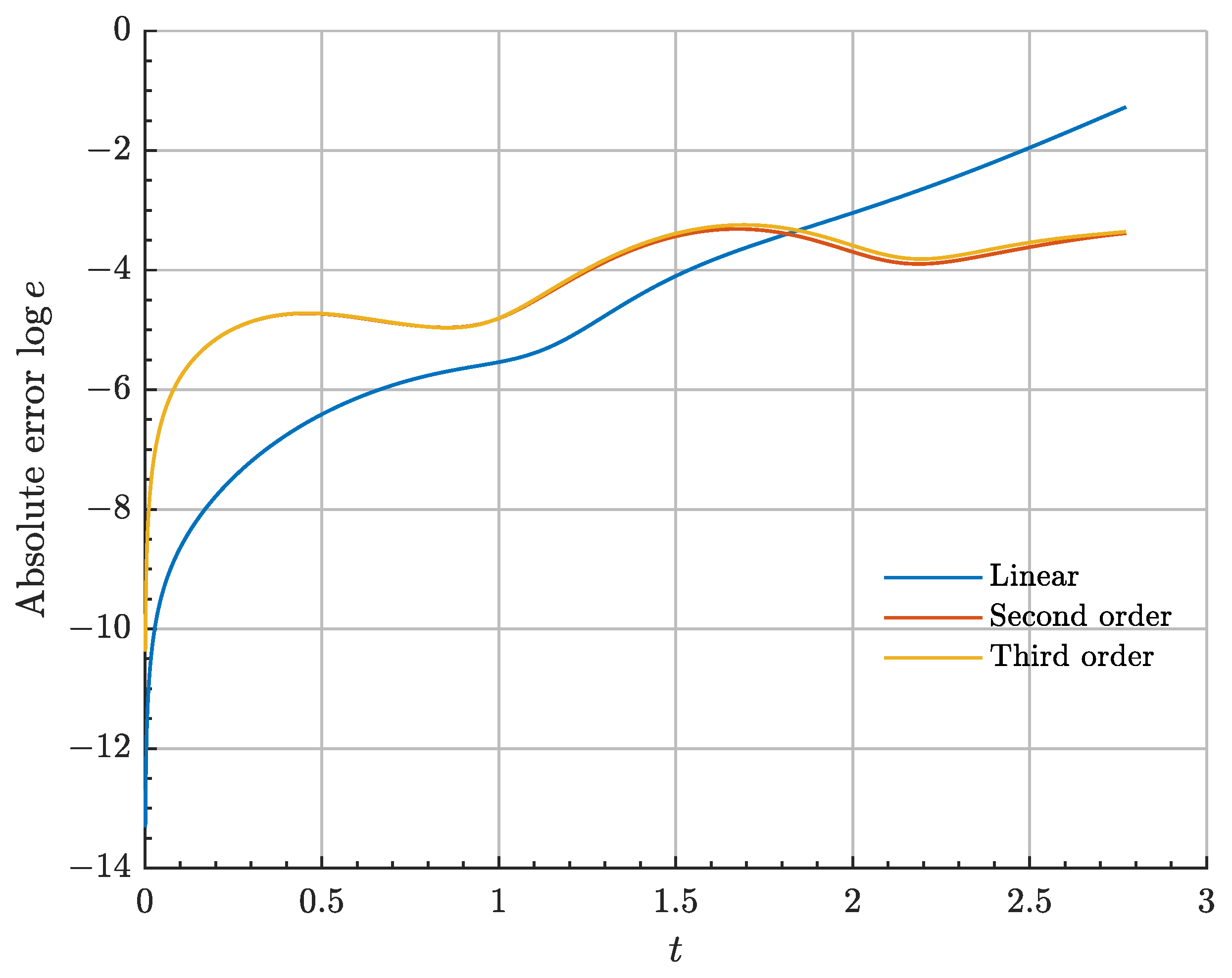
The following practical example provides a qualitative comparison between the accuracy of the three reduced-order models presented in this work against the full nonlinear dynamical model. The figure of merit in use is the
norm of the state error between the reconstructed chaser motion via LPO dynamics (implementing a differential corrector for increased accuracy) and via the different co-orbital motion models.
where
and
denote, respectively, the absolute chaser and target state (synodic components of the Cartesian position and velocity).
In the following application example, the target spacecraft is located in an Earth-Moon
standard halo orbit of out-of-plane amplitude of 20,000 km. The initial conditions of both the target and relative state are given by
Integration of the models is performed numerically for an orbital period of the chaser periodic orbit. The accuracy of the three different models is depicted in
Figure 2. As may be observed, while the linearized model is locally, for short time scales, the best approximation of the true co-orbital motion, higher-order models provide better performance when capturing long-term, nonlinear dynamics.
2.6. The Relative Libration Linear Dynamics and Inherited Normal Form
Much of the work to be derived in the following is founded on our last result regarding Equation (
12). In brief, if the spacecraft co-orbital motion near the collinear libration points is described by the well-known Richardson’s solution, its associated solutions also inherit (to the first order) the very same structures, such as quasi-periodic orbits and invariant manifolds. This conclusion is supported by dynamical system studies on the surveillance of the intrinsic transport phenomena under periodic perturbations, such as in our case, wherein the target motion acts as a periodic perturbation to Richardson’s potential [
71].
A definite proof of the inheritance of such orbital structures near the CR3BP phase space equilibrium points is given by the the normal form of the second-order relative Hamiltonian
Now, the relative angles
may be expanded under the condition
, where
still holds. Mathematically, this applies for near rendezvous scenarios at the
and
collinear points, reading
Retaining terms up to order
in the Euclidean norm of the relative primaries
yields
Plugging this result into the definition of
and again retaining first-order terms gives
which does not depend on the primary of interest
.
A similar procedure can be used to recover the classical frequency
from its time-dependent relative analogy
, using Newton’s generalized binomial theorem
Retaining the first-order term in the series expansion yields the desired result by definition [
7]
Finally, combining both approximations leads to the relative second-order Hamiltonian taking the form
which shares exactly the same normal form of the absolute Hamiltonian near the libration points. This result is necessary to theoretically support the Relative Libration Linear Model.
Following a similar argument to that given in [
9,
10], by means of a canonical transformation defined by the eigen directions of the relative STM, the Hamiltonian is set into the following form (in new coordinates
)
showing that the Rendezvous Condition near a libration point has saddle × center × behavior, generating relative periodic and quasi-periodic motions as for the LPO dynamics, with periodic time-varying planar and vertical frequencies
,
and stable and unstable relative motion directions characterized by
. The tuple
corresponds to the eigenvalues of the relative STM, linearized at the Rendezvous Condition [
10].
The existence of relative center, stable and unstable modes in the CR3BP have recently also been introduced quantitatively by Colombi, Colagrossi et al. [
53,
54,
55] and Zuelkhe et al. [
59,
60], but without explicit analytical support from the equations of motion. This result has also been well-studied in [
62] for spacecraft relative motion in the Keplerian problem. In this latter case, the center manifold is nothing but the traditional elliptic cylinder in which the Chief Circular Orbit is found.
For the sake of demonstration, a family of relative quasi-periodic orbits emerging from target–chaser halo motion in the Earth–Moon system is depicted in
Figure 3. Recent work [
60] has proposed classical differential correctors to compute naturally closed periodic orbits in the relative phase space, providing practical applications of the theoretical foundations here presented.
The relative time-dependent center manifold is given by
In virtue of the RLLM, Equation (
12), a first-order approximation for neutrally stable relative motion
, is given by a Lissajous curve [
8]
where
and
depend on the initial conditions of the relative state and the constants
are a function of the gravitational parameter
(or equivalently,
) and possibly time through the target’s motion. In reality, the periodic or quasi-periodic target motion
plays the role of a bifurcation parameter in this complete analysis. However, to our advantage, in the context of LPOs, disregarding the non-autonomous nature of such constants is generally valid as a first-order solution, uncoupling the relative state motion from the target state unknown time law. This geometrical reparametrization of the relative motion opens the door to quasi-analytical feedback guidance schemes [
65].
3. Optimal Relative Floquet Stationkeeping
This section is dedicated to the development of optimal stationkeeping schemes that exploit the natural CR3BP relative dynamics and their associated low-order structures revealed in the preceding section. A novel low-thrust algorithm is presented, featuring reduced order Floquet Theory.
Stationkeeping refers to the maintenance of an orbital state of interest, nullifying the effect of disturbances. Under the introduction of a virtual target spacecraft following a reference orbit, , the stationkeeping problem may be straightfordwardly reformulated as a regulation of the relative state between the target and chaser , and, therefore, as a Rendezvous Problem, subject to general optimization constraints.
Traditional stationkeeping algorithms have heavily relied on Floquet Theory to nullify the unstable nature of LPO under motion dynamics [
9,
15]. However, it was not until recently that the same principles started to be applied for relative co-orbital motion in the CR3BP [
65], under the formulation of which the stationkeeping problem transforms into a generic Rendezvous Problem. In the following, a reduced-order, optimal stationkeeping algorithm is developed, based on the relative Floquet transformation for general quasi-periodic LPO.
The original Floquet Mode Stationkeeping Scheme was developed by the Barcelona Group in their reformulation of the CR3BP under a Dynamical Systems Theory perspective [
9,
10,
15]. The algorithm directly exploits the dynamical structure of periodic orbits in the CR3BP to reduce long-term divergence from the nominal trajectory. This orbit deviation is always expected, due to the existence of an unstable hyperbolic manifold asymptotically departing from periodic orbits in forward time, as seen in
Section 2. Any initial perturbation with a non-zero component in the unstable direction exponentially grows in time, providing the major source of error from the target orbit (i.e., the reference orbit). Initial deviations along the center and stable manifolds, on the other hand, remain periodic or exponentially vanish, respectively. Therefore, it is the unstable manifold that is most concerning for stationkeeping applications.
The unstable manifold is locally defined by the eigenspectrum of the STM associated to the nominal reference orbit, or the corresponding Floquet Matrix. As first noted by Floquet [
72,
73], the Monodromy matrix admits the following decomposition:
in which both
and
J are constant in time. The former is known as the Floquet modal matrix and characterizes the eigenspace of the Monodromy matrix or Floquet directions and the general Jordan form,
J, is formed by the associated Floquet exponents and characterizes the system fundamental frequencies.
The Floquet basis vectors,
, and their associated exponents,
, relate to the eigenvectors
and eigenvalues
of the STM through the following expressions:
where
T is the orbital period. While the Monodromy representation of the dynamics may be used to characterize the invariant sets of the reference orbit, its Floquet counterpart is preferred, due its stable numerical behavior.
The transport of the time-dependent STM along the orbit of reference is, therefore, accomplished through
where
is also
T-periodic.
Provided that the Monodromy matrix exists, and in virtue of the Floquet Theorem, as seen in the previous section, a similarity transformation exists (given by
) such that the linear dynamics of the relative problem, Equation (
12), become
In such a representation, the major source of orbital error is given by the linear, uncoupled dynamics of the unstable component in the Floquet basis
, which traditional stationkeeping algorithms in the CR3BP aim to nullify [
9,
15,
74]. As already discussed, while previous developments have focused on formulating stationkeeping concerns as absolute dynamics tracking problems, where a reference trajectory, i.e., the reference orbit, is followed, it is more naturally understood as a regulation control problem of a relative system.
Some control policy may lead to the regulation of the relative state and, therefore, to the fulfilment of the stationkeeping problem. However, despite having been omitted, the Floquet transformation is time-dependent, Equation (
16), reading a linear-time varying dynamical system for which classical optimal results, such as the LQR, do not suffice without linearization or operation points techniques.
Still, the linear nature of the Floquet dynamics suggests the use of a state-dependent Ricatti Equation (SDRE) controller [
75] to asymptotically regulate such relatively unstable components, while suboptimally minimizing the control effort needed. A naive implementation of such an optimal policy would yield the closed-loop system
for the unstable control input vector
and feedback policy
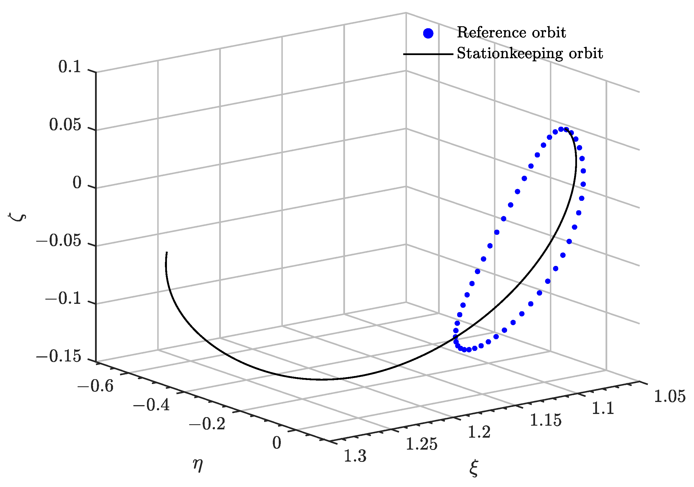
. However, while the Floquet uncoupled dynamics allow for an SISO system, underactuation along the center manifold of the orbit of interest, when mapped back to the original relative phase space, results in the spacecraft departing away from the reference trajectory. While the unstable component may be nullified, the central relative modes may be excited by the control law, leading the system to departure in the relative orbital family continuation direction. Such an effect is shown in
Figure 4, where the divergence of the spacecraft from its nominal orbit is clearly noticeable, despite the relatively unstable state component being regulated to 0.
In the CR3BP phase space, and by means of Lyapunov’s Theorem, the LPOs form one-parametric families, given [
64,
76]. Usually, either the Jacobi Constant
C or the orbital period
T are defined as continuation parameters of the family. When fulfilled, the stationkeeping problem ensures the convergence of both towards given reference values,
. Therefore, in this work, they were leveraged as additional relative state components to tie the SDRE-regulated relative solution to the original absolute LPO of interest, constraining the co-orbital state to remain in the original vicinity, while regulating the diverging state component. In practice, due to the lack of an analytical expression of
T as a function of the state components, only the Jacobi Constant is employed.
In this way, motivated by Koopman Control [
77,
78], the unstable Floquet coordinate system is coupled with the imposition of a Jacobi Constant error constraint, such that the resulting controlled plant follows a (neutrally) stable trajectory in the relative phase space with respect to a reference trajectory of energy
. Such constraint ensures that at any moment the LPO of reference is energetically accessible, a necessary condition for transport phenomena in the CR3BP. This strategy, hybridizing classical feedback and energy-shaping control, is particularly interesting for low-thrust propelled vehicles, which lack the impulsive capabilities that classical CR3BP stationkeeping algorithms rely on.
In particular, defining the energy error as
, the SDRE problem is established for the following dynamical system:
Matrix
is defined as the gradient of the Jacobi Constant with respect to the relative Floquet coordinates in time:
where
is the gradient of the Jacobi Constant with respect to the absolute chaser state
.
Finally, as the system is, in the general case, non-autonomous, the explicit evolution in time of the basis
F is computed through the relative STM Floquet decomposition or Equation (
16), together with the evolution of the Floquet coordinates
. In this sense, the analytical models presented for the relative motion in
Section 2 are of particular interest. Moreover, it is usually also reasonable to take the reference orbit STM as that of the relative motion.
For online performance, the LTI version of the problem can be leveraged using gain-scheduling techniques or linearizing the problem around the Rendezvous Condition, so that the LQR may be directly used.
Stationkeeping Examples
The demonstration of the novel stationkeeping algorithm was accomplished in an Earth–Moon
scenario. In particular, stationkeeping maneuvers were performed for a spacecraft target located in a southern halo orbit of out-of-plane amplitude
30,000
, as given in [
26]. The absolute initial conditions in the reference orbit are
However, such an initial state is subject to insertion errors in both position and velocity space, which follow appropriate normal distributions. The initial relative state is, therefore, modeled as
where the standard deviation is of
in position and
in velocity space, which are similar values to those used in [
26], while providing really unstable initial insertion conditions. For the mission considered, at first, the following relative initial conditions are used
which corresponds to an initial range of
.
The stationkeeping Floquet controller is defined by the following penalty matrices
which are held constant and trade-off both control expenses and final stationkeeping error.
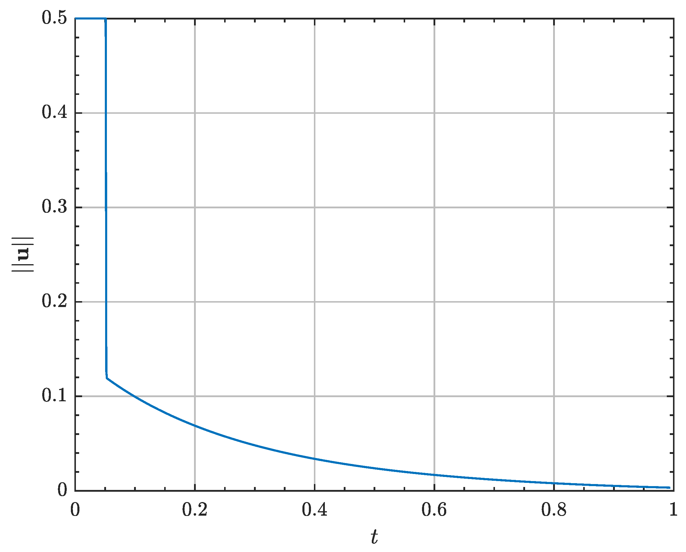
The selection of the matrices was achieved heuristically, to maintain the generality of the results. Moreover, the execution of maneuvers was only performed for 30% of the total orbital period, at the perilune, after insertion. Maximum acceleration was constrained to be less than . The mission duration was of non-dimensional units, which corresponded to an orbital period of the reference halo orbit.
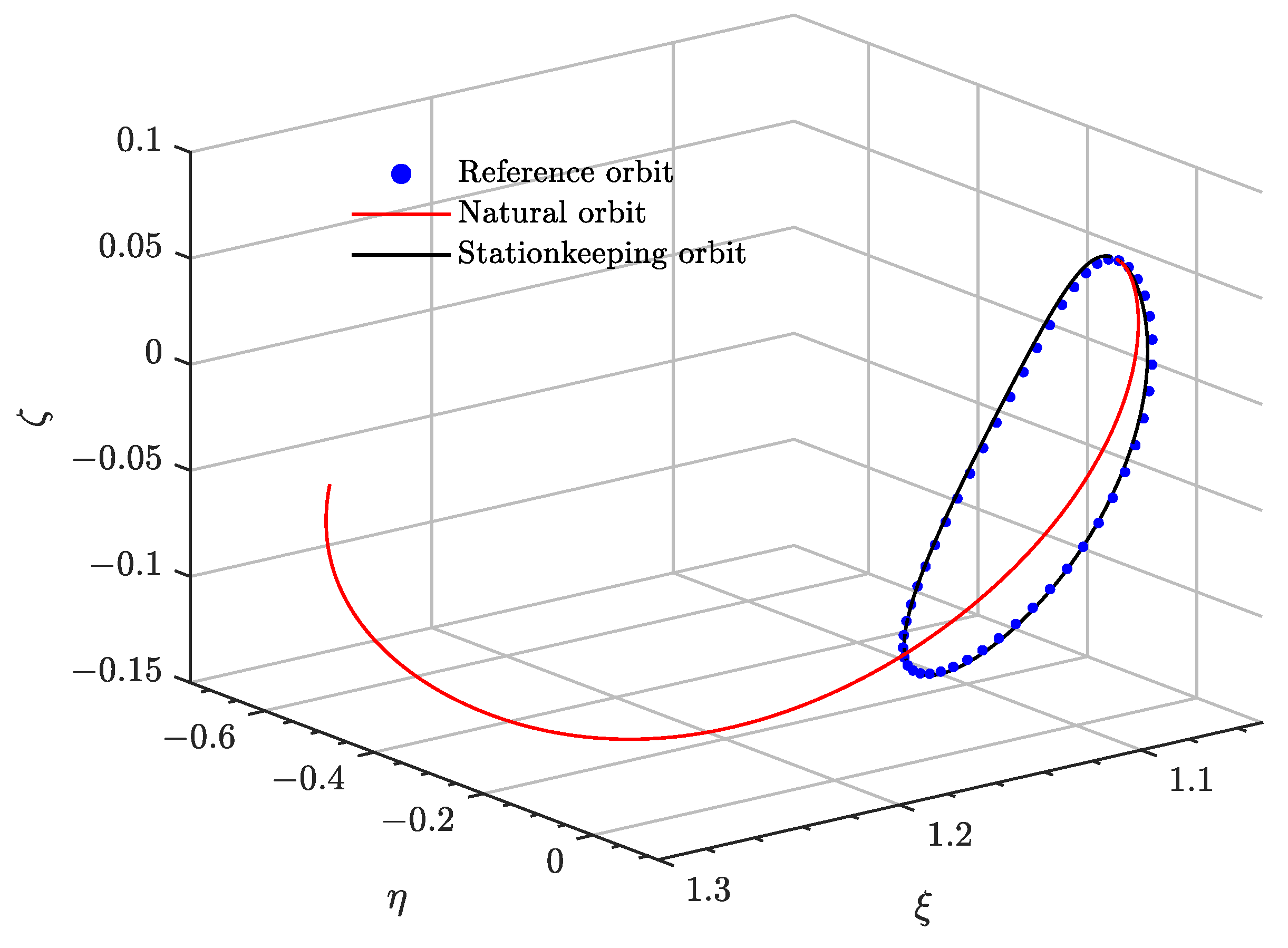
Despite these limitations, as seen in
Figure 5 and
Figure 6, the algorithm was able to maintain the vehicle in the nearbies of the reference orbit. In the absence of stationkeeping maneuvers, the target naturally diverged to the Earth–Moon realm due to the effect of the insertion and navigation errors.
Figure 7 depicts the control acceleration needed during the stationkeeping phase.
Table 1 summarizes the main performance metrics for the mission, showing great efficiency in maintaining the relative state close to
without major control expenses. Moreover, it also compares the performance of the algorithm time-invariant version (LQR), which exploits local linearization of the Floquet eigenbasis around the Monodromy matrix of the orbit, and the target’s insertion phase space vector. The execution of the LQR policty was, however, restricted to 10% of the orbital period
T, around which the operating point linearization was valid.
From the results obtained, it is clear that both the SDRE and its simplified, time-invariant LQR version, performed really closely, in terms of control cost, while the LQR showed a 50% reduction in terms of error integrals and an order of magnitude computational speed which was up when the same time of flight was considered. However, it had a local region of applicability. In both cases, the algorithm was able to maintain the spacecraft orbit near its reference motion at really low control expense and acceleration values. Moreover, it benefited from a reduced-order structure (exploiting simple relative dynamics structures and arguments), which has interest not only theoretically, but also for real, embedded time implementation purposes.
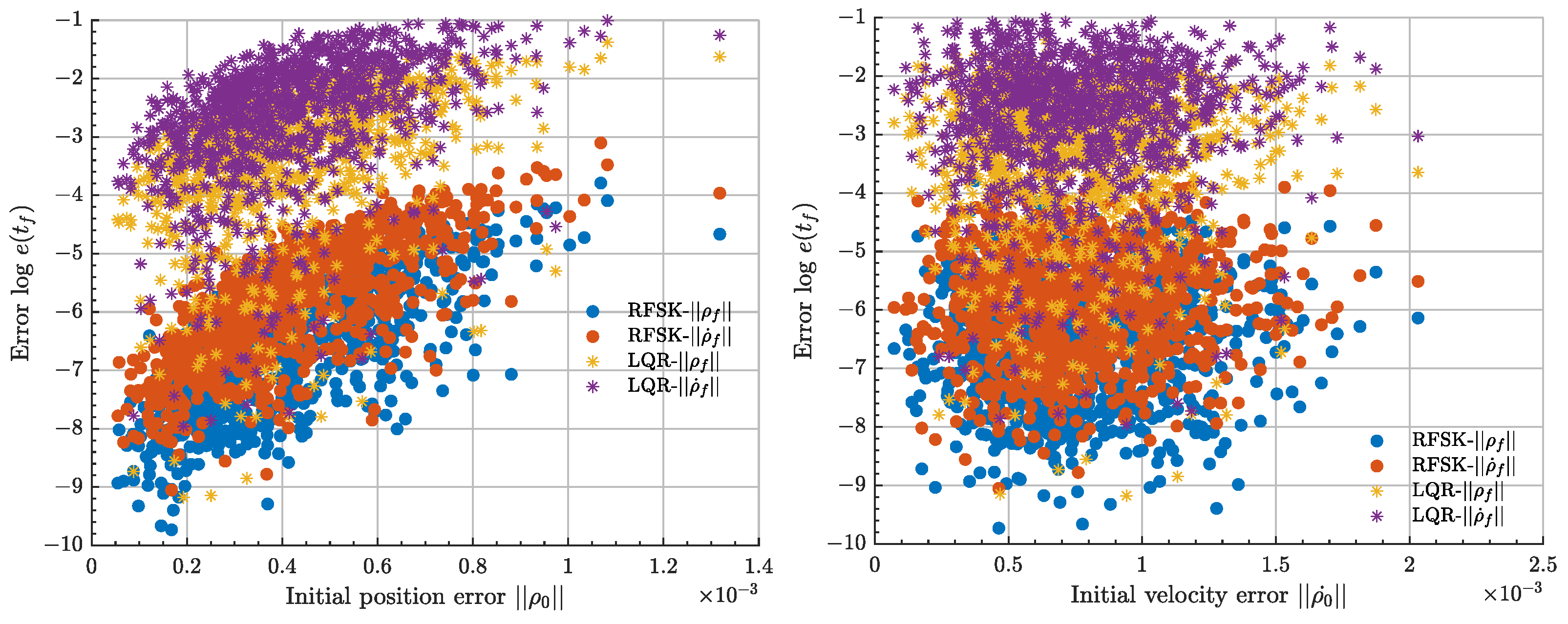
The performance of the algorithm was further investigated in a Monte Carlo simulation of 1000 draws for the very same orbital configuration and parameters. The initial relative phase space vector (corresponding to the halo initial position and velocity errors) followed component-wise normal distributions with null mean and standard deviations of and , for position and velocity, respectively.
Comparison against a similar LQR (including an integral penalty term [
38]) to that presented in [
26] was also addressed. The operating point of the controller was selected to be the reference initial phase space vector of the reference halo. The defining penalty matrices for such a controller were selected to be
corresponding to the same order of magnitude of those used in [
26]. To ensure the validity of the results obtained, the RFSK algorithm was implemented in its linearized form around the nominal insertion point.
Figure 8,
Figure 9 and
Figure 10 address the comparison between the two controllers, in terms of control cost and final relative phase space error (in position and velocity), as a function of the initial relative error to the target halo. Computational resources needed for each algorithm were also considered.
As can be seen, both algorithms performed really closely in terms of computational cost. However, for the same considered stationkeeping time of flight, the novel RFSK was clearly outstanding in terms of final relative position and velocity error, while providing, at worst, the same control cost as that of the LQR. Given such results, the RFSK algorithm is a clear substitute to classical LQR regulating techniques.


