
Short-Arc Horizon-Based Optical Navigation by Total Least-Squares Estimation

1
Micro-Satellite Research Center, School of Aeronautics and Astronautics, Zhejiang University, Hangzhou 310027, China
2
Zhejiang Key Laboratory of Micro-Nano Satellite Research, Hangzhou 310027, China
*
Author to whom correspondence should be addressed.
†
These authors contributed equally to this work.
Aerospace 2023, 10(4), 371; https://doi.org/10.3390/aerospace10040371
Submission received: 7 March 2023
/
Revised: 7 April 2023
/
Accepted: 11 April 2023
/
Published: 13 April 2023
(This article belongs to the Special Issue Advanced Spacecraft/Satellite Technologies)
Abstract
:Horizon-based optical navigation (OPNAV) is an attractive solution for deep space exploration missions, with strong autonomy and high accuracy. In some scenarios, especially those with large variations in spacecraft distance from celestial bodies, the visible horizon arc could be very short. In this case, the traditional Christian–Robinson algorithm with least-squares (LS) estimation is inappropriate and would introduce a large mean residual that can be even larger than the standard deviation (STD). To solve this problem, a simplified measurement covariance model was proposed by analyzing the propagation of measurement errors. Then, an unbiased solution with the element-wise total least-squares (EW-TLS) algorithm was developed in which the measurement equation and the covariance of each measurement are fully considered. To further simplify this problem, an approximate generalized total least-squares algorithm (AG-TLS) was then proposed, which achieves a non-iterative solution by using approximate measurement covariances. The covariance analysis and numerical simulations show that the proposed algorithms have impressive advantages in the short-arc horizon scenario, for the mean residuals are always close to zero. Compared with the EW-TLS algorithm, the AG-TLS algorithm trades a negligible accuracy loss for a huge reduction in execution time and achieves a computing speed comparable to the traditional algorithm. Furthermore, a simulated navigation scenario reveals that a short-arc horizon can provide reliable position estimates for planetary exploration missions.
1. Introduction
Autonomous navigation is being widely valued with the bloom of deep space exploration missions [1,2]. It is an effective supplement and backup for ground-based tracking to reduce ground maintenance costs, overcome communication delays, and prevent communication loss [3]. Optical navigation is an image-based solution with strong autonomy, high accuracy, and good real-time performance [4]. It has been successfully applied to interplanetary exploration missions such as Apollo [5], Deep Space 1 [6], and SMART-1 [7] and will soon be applied to Orion missions [8].
OPNAV comes in many forms, including extracting the line-of-sight direction of natural or artificial targets [9,10,11], using the horizon of a celestial body [12,13,14,15], and tracking the landmarks on the body’s surface [16,17,18,19]. The most appealing solution for a planetary exploration mission is the horizon-based OPNAV, which guarantees a good balance of accuracy and complexity. The position of the spacecraft can be determined by using the planet’s centroid and apparent diameter in the image [12]. In most applications, the OPNAV camera’s field of view (FOV) is carefully designed to exactly cover the entire celestial body for better navigation accuracy. However, in some cases, the visible horizon arc could be very short, for example, due to the influence of lighting conditions, deviation of the pointing angle, and, most notably, change in altitude. In a typical Mars exploration mission, the distance between the spacecraft and Mars varies from a few hundred kilometers to tens of thousands of kilometers [1]. To ensure full-stage navigation accuracy, the FOV of the navigation camera is generally small such that only a small part of the horizon or scenery can be captured at the perigee. Although landmark-based OPNAV techniques can provide higher accuracy, they imply additional modes of navigation sensors and higher computational requirements. Thus, OPNAV, which only relies on a short-arc horizon, is essential.
The perspective projection of an ellipsoid planet or moon is an approximate ellipse, so many ellipse fitting algorithms have been used for the problem of horizon-based OPNAV [12,20]. In some applications, the celestial body with low ellipticity is directly approximated as a sphere, resulting in a simple and robust solution at the expense of some accuracy [21,22]. The traditional method of direct ellipse fitting in the image plane will incorrectly converge and introduce large errors in the case of a short-arc horizon. To solve this problem, Hu et al. [23] takes ephemeris and the spacecraft’s position as prior information and simplifies the ellipsoid to a sphere, thus obtaining the size and shape information of the ellipse in the image plane beforehand. The fitting accuracy of a short-arc horizon is greatly improved because there are only two unknown pieces of information, a scalar of the ellipse’s rotation and a two-dimensional vector of the ellipse’s translation on the image plane, to be estimated. This approach is inappropriate for our application due to the lack of position information, but it still reveals the difficulty of short-arc ellipse fitting and the importance of using prior information. The state-of-the-art solution is the Christian–Robinson algorithm [13,24,25], in which the ellipsoid celestial body is transferred into a sphere through Cholesky factorization, thus leading to a non-iterative solution. This is undoubtedly a novel and elegant solution that makes full use of prior information and greatly simplifies the problem. It has been employed in evaluating various OPNAV missions and has shown excellent performance [21,26].
In the Christian–Robinson algorithm, it was mentioned that the measurement equations should be solved using either the least-square (LS) estimation or the total least-square (TLS) estimation, but no detailed analysis was given [25], and LS estimation has widely been used for its simplicity [21,24,26]. The ordinary LS estimation assumes that the basis function is error-free. However, in the measurement equation of the Christian–Robinson algorithm, the measurement errors are entirely embedded in the basis function . TLS estimation addresses errors in the matrix, thus obtaining higher estimation accuracy and smaller estimation bias than the LS estimation [27]. TLS estimation is an asymptotic unbiased estimator whose error covariance achieves the Cramér–Rao lower bound [28,29]. It has been widely used in various measurement and estimation applications and demonstrates excellent performance [30,31,32,33,34]. However, compared with LS estimation, TLS estimation is more complex to apply and brings a non-negligible time consumption. In addition, TLS estimation is a general term for a class of algorithms with many variants [35,36,37]. It is necessary to further analyze why and when TLS estimation is needed and how it is implemented.
In this paper, we concentrate on improving the performance of horizon-based OPNAV based on a short-arc horizon. The main contributions of this paper lie in the following aspects: (1) Theoretical analysis reveals that LS estimation applied to the traditional Christian–Robinson algorithm is inappropriate and may introduce estimation bias. (2) A simplified measurement covariance model is proposed by further analyzing the propagation of measurement errors. The covariance model is no longer limited by the narrow FOV approximation and can be adapted to large FOV cameras. (3) An unbiased solution with the EW-TLS algorithm is developed. By considering the measurement equation and the covariance of each measurement, mean residuals close to zero can be achieved. (4) To further simplify this problem, an AG-TLS algorithm is proposed, in which a non-iterative solution is achieved by using the covariance of any one measurement as an approximation of all measurement covariances. Compared with the EW-TLS algorithm, the AG-TLS algorithm trades a negligible accuracy loss for a huge reduction in execution time. Its computing speed is comparable to the traditional algorithm and is suitable for onboard applications. (5) Covariance analysis and numerical results prove that the covariances of the LS estimation and the TLS estimation in this problem are identical, and the difference between them lies in the possible estimation bias. Due to the drawbacks of LS estimation, the Christian–Robinson method with ordinary LS estimation introduces large mean residuals under a short-arc horizon scenario, while the EW-TLS algorithm can achieve near zero mean residuals.
The remainder of this paper is organized as follows. Section 2 reviews the horizon-based OPNAV problem. Section 3 analyzes the problem in detail at the theoretical level and describes the proposed algorithms using TLS estimation. Section 4 presents the results of numerical simulations, and the main conclusions are summarized in Section 5.
2. Brief Review of Horizon-Based Optical Navigation
2.1. Geometry Fundamentals
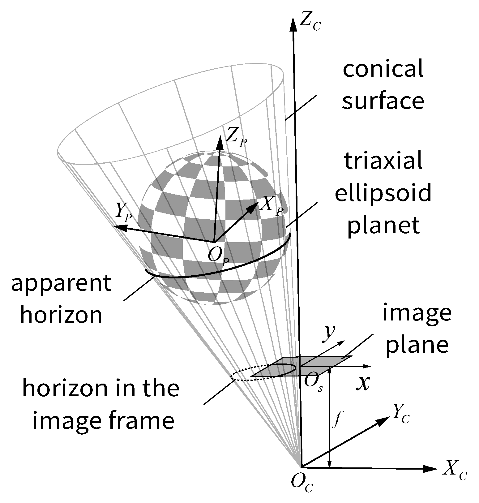
The geometry of horizon-based OPNAV is shown in Figure 1. When the navigation camera takes a picture of an ellipsoid planet, the vectors from the camera’s optical center to the planet’s apparent horizon will form an approximate conical surface that tightly bounds the planet. Here is a brief review of the geometry fundamentals behind this.
To clarify the statement, several reference frames are introduced, which are defined as follows. The planetary frame (P) is established with the center of the planet () as the origin. The X-axis(), Y-axis(), and Z-axis() of frame P are directions of the planet’s three principal axes, respectively. The origin of the camera frame (C) is the optical center of the camera (). The X-axis () and Y-axis () of frame C are directions of the row and column of the image sensor, respectively. The Z-axis () of frame C is normal to the plane. The image frame takes the imaging center of the image sensor () as the origin. The row and column of the image sensor are taken as the X-axis (x) and Y-axis (y) of the image frame, and the unit is a pixel. The image plane is right in the image frame, while its size is limited by the image sensor.
Note that the following analysis is performed in the camera frame C unless otherwise indicated. For an ideal navigation camera that perfectly follows the perspective imaging relationship [38], a detected planetary horizon point in the image frame corresponding to the following horizon vector :
where f is the focal length of the navigation camera in pixels. The shape of most regular planets can be approximately described by a triaxial ellipsoid, then all the apparent horizons form a conical surface tightly bounding the triaxial ellipsoid during the imaging process [12]. For any horizon vector belonging to the conical surface, it obeys the following constraints:
where is a full rank symmetric matrix. The expression of is as follows:
where is the position of camera center relative to planet center , and describes the shape and orientation of a triaxial ellipsoid. The expression of is as follows:
where represents the length of the planet’s three principal axis, and represents the rotation matrix from the planetary frame P to the camera frame C. With the development of high-precision ephemeris and star trackers, a high-precision can be easily obtained, which will serve as prior information for the entire problem.
2.2. The Christian–Robinson Algorithm
The Christian–Robinson algorithm makes full use of prior ellipsoid shape and camera attitude information. The algorithm transforms the triaxial ellipsoid into a unit sphere through Cholesky factorization, thereby fully simplifying the triaxial ellipsoid projection constraint. Here is a brief review of the algorithm.
- (1)
- Convert the camera’s horizon measurement to in Cholesky factorization space:where can be obtained from Equation (4) as:and the expression of is as follows:
- (2)
- Normalize to :
- (3)
- The problem is converted to solving for in the following measurement equations:where:, n is the total number of horizon measurement points.
- (4)
- The solution of could be found by:
3. Total Least-Squares Estimation
3.1. Estimation Bias Caused by Least-Squares Estimation
With the help of the Christian–Robinson algorithm, the problem has been greatly simplified to solving for in Equation (9). Although it was mentioned in [25] that the measurement equations should be solved using either the LS estimation or the TLS estimation, no detailed analysis was given. The LS estimation seems to bring the same results with much lower computational consumption in most cases, so it is more widely used [21,24,26]. However, the limitation of the LS estimation seriously affects the performance of the algorithm in short-arc horizon-based OPNAV. This will be demonstrated in the following derivations.
Let us revisit the problem described in Equation (9). If the problem is treated as a LS problem, then its loss function is:
where is the measurement of , is the measurement of , and is the LS solution. As shown in Section 2.2, is converted from the camera’s horizon measurement by Equations (5) and (8), is set as directly from Equation (9), and the expression of is:
If we treat as a function of the measurements, then the expectation of the LS solution is:
It can thereby be concluded that LS estimation is a biased estimation for this problem [27], and the estimation bias is:
Estimation bias is unavoidable in LS estimation due to the error contained in , and its existence is verified in subsequent simulations. The estimation bias will increase with the lack of measurement information due to the shortening of the horizon arc length. In practice, estimation biases are not easily detected without additional correction methods. Furthermore, it is undoubtedly catastrophic for subsequent Kalman filter or other estimation frameworks if the estimation bias is large enough compared with the estimation error.
3.2. Simplified Measurement Covariance Model
As shown in the last section, the key to the estimation bias is the coupling of the measurement error with the measurement model. To solve this problem, we need to find out the covariance of measurement errors beforehand, which means studying the propagation of the measurement error in the transition of horizon measurements in the image to in the measurement model. The narrow FOV approximation was used in previous covariance derivations, which greatly limited its applicability [20,24,39,40]. In this paper, a more general and simple measurement covariance model is given by reducing the normalization step of the measurement vector.
At first, a detected horizon point in the image frame describes the horizon point’s line-of-sight direction. The measured error should be uniformly Gaussian distributed in the image plane, then the covariance of can be expressed as:
where is the STD of the horizon point location error, and the unit is one pixel.
Then, the covariance changes during the projection of the point in the image frame to the vector in the camera frame C. The narrow FOV approximation is commonly used to estimate the covariances of when the camera has a small FOV [20,24]. A small FOV indicates that the focal length f is much greater than the size of the image sensor, allowing for the assumption that the covariance of any normalized within the narrow FOV remains constant [40]. However, we do not use the narrow FOV approximation in our covariance model because it would restrict the model from being applied to cameras with larger FOVs. Instead, we apply the normalization step only once at a later stage. This approach further simplifies the covariance calculation and increases the model’s versatility. The projection corresponds to the Jacobi matrix as follows:
Thus the covariance of is:
Due to the characteristics of camera measurements, the covariance of is not uniformly distributed in three directions, and the errors mainly accumulate in and directions. Note that a more general theory of camera measurement covariance could be found in [39], while the one used here is an adequate simplification.
Next, consider the transformation corresponding to Equation (5), in which in the camera frame P is transferred into in the Cholesky factorization space. The transformation corresponds to the Jacobi matrix as follows:
In addition, as shown in Equation (8), the vector needs to be normalized to . The normalization corresponds to the Jacobi matrix as follows:
Defining the matrix thus obtains:
Since the magnitude of every measurement is different, the covariance of each measurement varies after normalization.
Finally, the covariance of is found to be:
3.3. Element-Wise Weighted Total Least-Squares Algorithm
As shown in the previous section, the measurement error propagation leads to different covariance for each measurement. In addition, the measurements act as a model in the measurement equation, which means that this is an entirely error-in-variables problem. To better address this problem, the TLS estimation is adopted, which takes into account the error in the matrix and weights the measurement equations based on the covariance of the measurements.
For this problem, define the following matrix:
The constraint condition Equation (9) can then be rewritten as:
TLS solution for this problem is the optimal estimation of that minimizes [28]:
where denotes the estimation of , denotes the measurement of , denotes the estimation of , denotes the estimation of , is the covariance matrix of , and vec denotes a vector formed by stacking the consecutive columns of the associated matrix. is given by following block diagonal matrix:
where is covariance matrix of , and it is given by:
As defined in Equation (15), there is:
In this case, since the errors are element-wise correlated and non-stationary, each measurement element needs to be weighted according to its covariance. It implies that this is an element-wise weighted TLS (EW-TLS) problem and can be solved by using an iterative procedure [27,36]. In addition, it is necessary to impose strict time limits on the algorithm to ensure implementation onboard. The specific steps of the EW-TLS algorithm are as follows:
- (1)
- Calculate the covariance of each set of measurements with Equation (25).
- (2)
- Take the LS estimation as the initial estimate with Equation (13).
- (3)
- (4)
- The iteration is stopped when the final change is less than the tolerance value, or when the number of iterations is greater than the maximum number of iterations (MaxIterations). The iteration stopping conditions are specified as:
The tolerance value is set according to the calculation precision, and it is set to in this paper. MaxIterations is limited to five to avoid excessive time consumption. Although it is certainly satisfactory that the algorithm usually converges in only one to three iteration cycles, it is definitely safer to impose a limit on the number of iterations.
3.4. Approximate Generalized Total Least-Squares Algorithm
Although the accuracy of the EW-TLS algorithm is satisfactory, its computation time is still too long. Considering the limitations of onboard computing capabilities, it is usually worthwhile to trade some precision loss for faster computation. To further simplify this problem, an AG-TLS algorithm is proposed in this paper, which uses the covariance of any one measurement as an approximation of all covariances, thus achieving a non-iterative solution.
Recall the analysis of measurement error propagation in Section 3.2. For a planet with a small oblateness, its three major axes a, b, c are very close, and Equation (6) can be approximated as:
where is the mean radius of the target planet. Thus, may be rewritten as:
The attitude transformation matrix does not change the norm of , which lead to:
For a narrow FOV camera, the focal length f is much larger than and is approximately:
As shown in Equation (21), is constant and mainly accumulated in and directions. Then, as shown in Equation (42), when horizon measurements in the image transitions to in the measurement model, are redistributed to three directions with . The variation of is dominated by the variation of , while changes relatively little since all measurements are gathered in a small area for a narrow FOV camera.
According to the above analysis, it can be concluded that when both camera’s FOV and planetary oblateness are small, are relatively close for all measurements . Therefore, the problem can be further simplified with a small loss of precision by taking the covariance of any one measurement as an approximation of all covariances. Considering the error distribution and correlation among the elements, the simplified problem is a generalized TLS estimation problem, which has a closed-form solution [27,35,36]. The specific steps of the AG-TLS algorithm are as follows:
- (1)
- (2)
- Prepare for Cholesky factorization of matrix . According to Equation (32), should be equal to zero, while this will lead to a rank deficient of . In addition, the covariance matrix is a positive semi-definite matrix. With the change in spacecraft position and attitude, and considering the machine computational accuracy, will sometimes have an eigenvalue close to zero or even negative. These factors block the Cholesky decomposition of the matrix and affect the implementation of the algorithm. Thus, the approximate covariance matrix is obtained by making a simple but effective adjustment to .where is a very small value, e.g., , and is much smaller than every element in the matrix . Such an approximation hardly affects the distribution of covariances and ensures that the matrix is positive definite.
- (3)
- Perform a Cholesky factorization on the matrix :Then partition the inverse of as:where is an matrix, is an vector, and is a scalar.
- (4)
- Perform a singular value decomposition on the following matrix:Then partition as:where , and are matrixes, is an matrix, is a scalar, and and are both vectors.
- (5)
- The final solution is given by [27]:
3.5. Analytic Solution Covariance
In this section, the analytic solution covariance of the TLS estimation and the LS estimation are evaluated to compare their performance under this problem.
According to [28], the analytic solution covariance of with TLS estimation is:
According to Equation (32), it can be simplified as:
So the analytic solution covariance of is:
The analytic covariance of with LS estimation is:
Since is assumed to be unperturbed in the ordinary LS estimation, there are:
Therefore, it can be obtained:
That is to say:
It can be seen that the analytic covariances of the LS estimation and the TLS estimation are completely consistent, then the difference between the two kinds of estimations lies in the possible estimation bias. As demonstrated in [28], the TLS estimation is asymptotically unbiased, which is the main advantage over the ordinary LS estimation in this problem, so it is certainly attractive to adopt the TLS estimation without any loss of precision. In the actual performance of the EW-TLS algorithm, the analytic solution covariance will be gradually approximated as the iteration number grows, while in the AG-TLS algorithm, there may be a gap between the actual performance and the analytics solution covariance due to the presence of approximations. The actual performance of the proposed algorithms is verified in the following numerical simulations.
4. Numerical Results
4.1. Performance under a Short-Arc Horizon
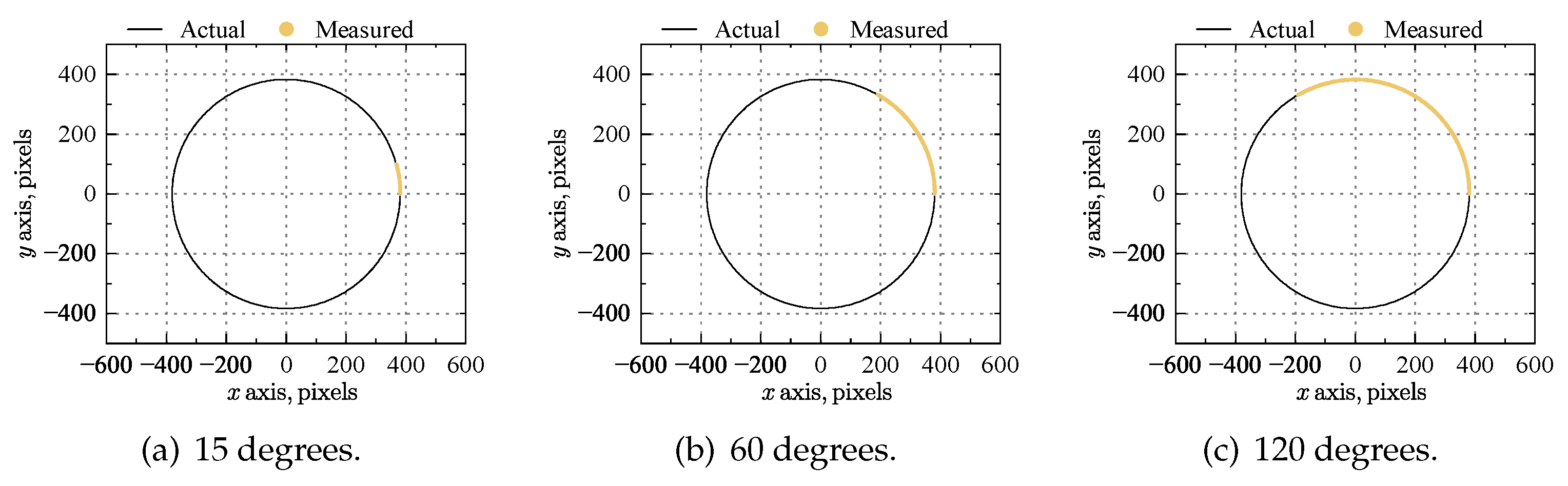
The simulated navigation camera assumed a FOV of 8x8 degrees and a resolution of 1024 × 1024 pixels. The exact numerical solution of the apparent horizon in the image plane could be found using Equations (1)–(3). One horizon point is sampled from each pixel where the horizon appears, and Gaussian distributed errors with pixel are added to the horizon points, thus getting closer to the actual horizon detection situation. The above simulation conditions of navigation camera are applied to all subsequent simulations. The simulated navigation camera is pointing to the center of Mars at a range of 65,000 km. At this point, the horizon of Mars occupies almost the entire FOV of the navigation camera. However, due to the possible deviation of the pointing angle and the influence of lighting conditions, only a small part of the horizon may be detected. Simulated images of the horizon ellipse with different arc lengths in the image frame are shown in Figure 2.
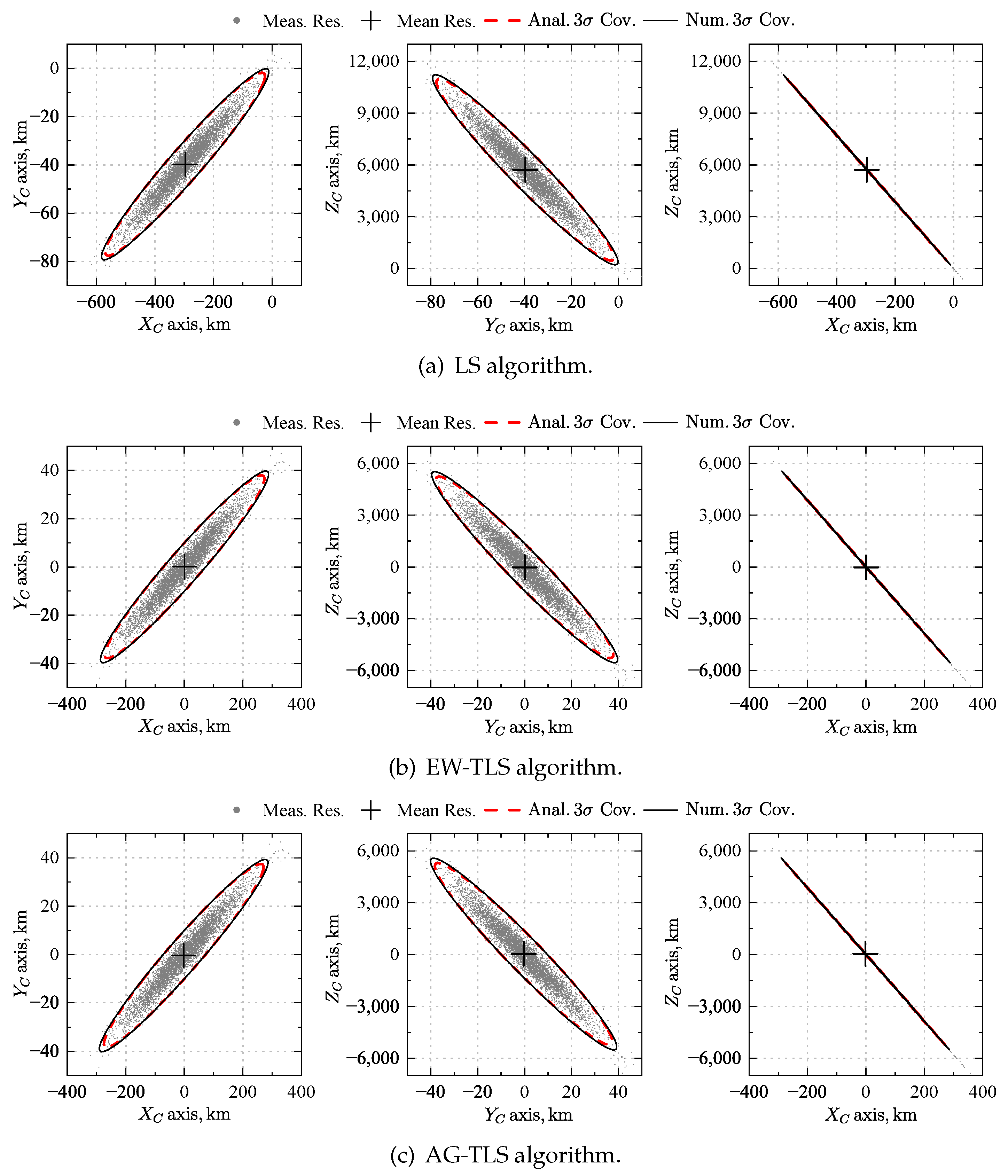
As an example scenario, assume that a 15-degree of horizon arc is detected, and the actual number of valid horizon points is about 100. For convenience, the Christian–Robinson algorithm with LS estimation is called the LS algorithm, while the algorithms proposed in this paper are called the EW-TLS algorithm and AG-TLS algorithm. A total of 5000 Monte Carlo simulations are performed with three algorithms. Various horizon measurements are produced by adding randomly generated Gaussian noise to the same scenario, and the results are shown in Figure 3. Errors of OPNAV are presented in the camera frame C. Gray points represent measurement residuals of Monte Carlo simulations, the black cross represents mean residuals of simulations, the red dashed line ellipse represents 3 bounds of analytic covariance, and the black solid line ellipse represents 3 bounds of numeric covariance from simulations. Note that the covariance in Figure 3 is superimposed on the mean residuals. In the simulations of all three algorithms, the analytical covariance and the numeric covariance are in good agreement, and the correctness of the analytic covariance is fully verified.
The detailed results of Monte Carlo simulations are listed in Table 1. The magnitude of the solution covariances is the same for all three algorithms. However, as shown in Figure 3a, the mean residuals of the LS algorithm are clearly not zero. The mean to the standard deviation ratio (MSTDR) is introduced here to evaluate the influence of mean residuals. MSTDR is set to be a positive value. MSTDR of the LS algorithm in , , and directions are 311.63%, 301.23%, and 311.67%, respectively. This means that the mean residuals are much larger than the STD, which is unacceptable in practical applications. In contrast, as shown in Figure 3b,c, the MSTDR of the EW-TLS algorithm and AG-TLS algorithm are all near zero. The root mean squared error (RMSE) is introduced to evaluate the estimation effectiveness of all three algorithms with respect to mean residuals, and two TLS algorithms both show a significant accuracy advantage of three times over the LS algorithm. The mean residuals of the AG-TLS algorithm are slightly larger than the average error of the EW-TLS algorithm. From the perspective of MSTDR, the performance difference between the two algorithms is within 2%, while it is basically no different from the perspective of RMSE, which indicates that the approximation and simplification of the AG-TLS algorithm are effective under a short-arc horizon.
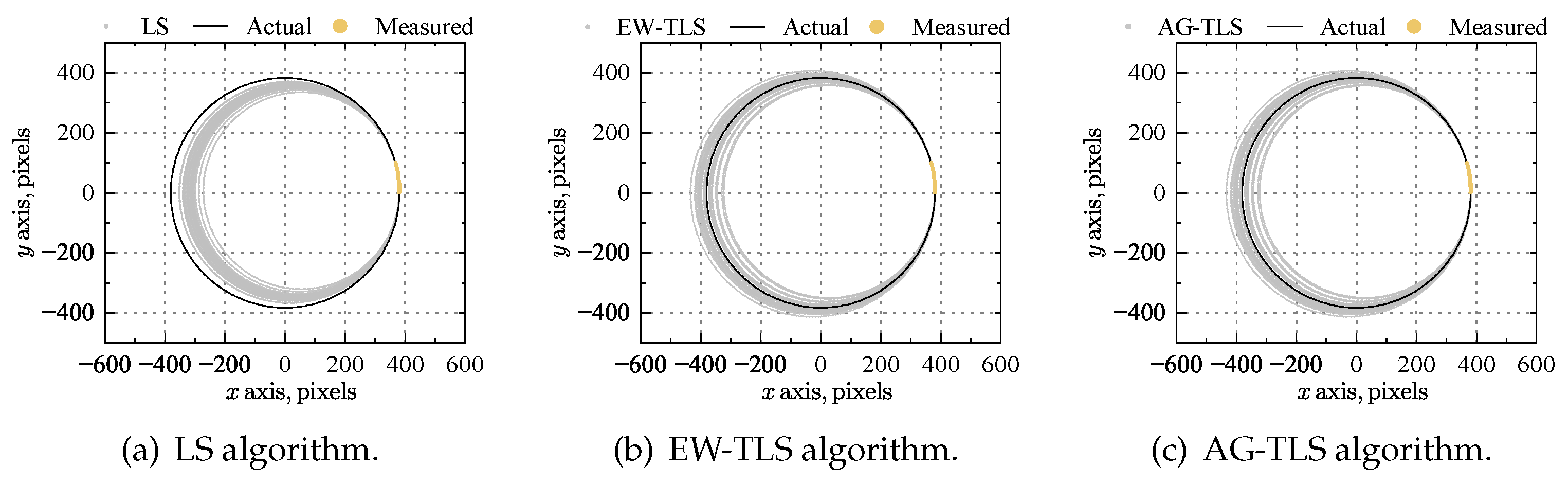
Although there is no circle fitting or ellipse fitting of the projected horizon in the image frame in the Christian–Robinson algorithm, it is still more intuitive to use the projected horizon in the image frame to show the solution results. Substituting the true value of , LS algorithm’s estimation of , EW-TLS algorithm’s estimation of , and AG-TLS algorithm’s estimation of into Equations (1)–(3) yields the actual projected horizon ellipses, LS-projected horizon ellipses, EW-TLS-projected horizons, and AG-TLS-projected horizon ellipses in the image frame, respectively. These ellipses are shown in Figure 4 together with the measured horizon arc. Compared with the actual projected horizon ellipse, LS-projected horizon ellipses are generally offset and relatively small, which means that the distance from the camera to the planet estimated by the LS algorithm is larger than the actual value, and there will be a direction error. On the contrary, EW-TLS-projected horizon ellipses and AG-TLS-projected horizon ellipses can both basically fit the actual projected horizon ellipse. This is consistent with our previous analysis that the LS estimation introduces a non-negligible bias, while the TLS estimation eliminates the effect of the bias.
4.2. Performance under Different Horizon Arc Lengths
More Monte Carlo simulations are conducted to evaluate the algorithms’ performance under different lengths of detected horizon arc. The actual number of valid horizon points increases linearly with increasing arc length. A total of 5000 sets of independent simulations are conducted for each experimental condition. Various horizon measurements are produced by adding randomly generated Gaussian noise to the same scenario, and the results shown are the average values of these measurements. Errors of OPNAV are presented in the camera frame C. RMSE and MSTDR are used to evaluate the performance of three algorithms.
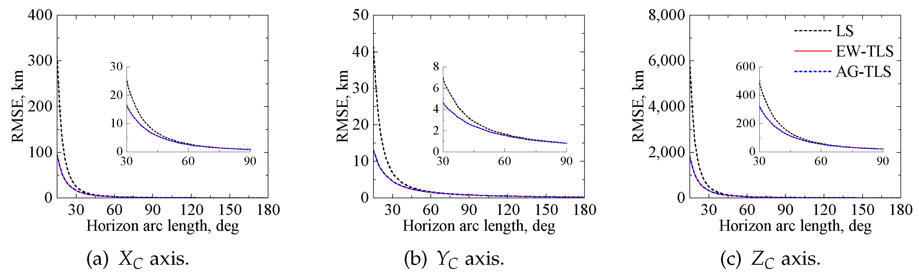
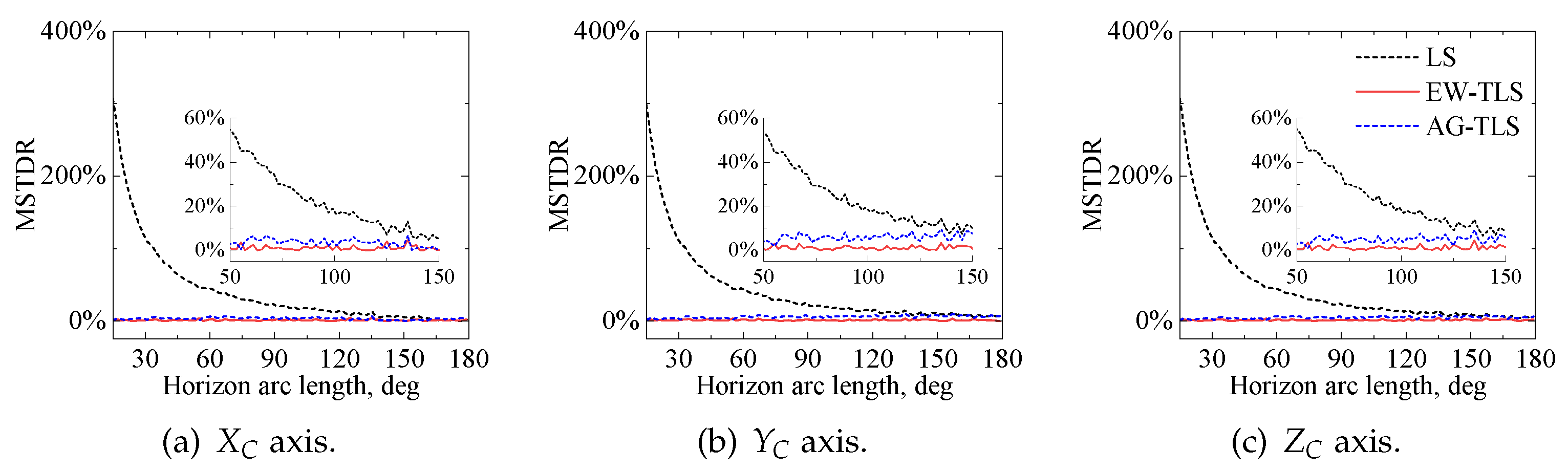
The results of the simulations are shown in Figure 5 and Figure 6. The RMSE of the three algorithms gradually decreased as the arc length was increased, which is consistent with the previous study of horizon-based OPNAV covariance [41]. At the same time, the gap between the RMSE and MSTDR between the LS algorithm and the TLS algorithms also decreased. As seen in Figure 5, both the EW-TLS algorithm and AG-TLS algorithm show great advantages over the LS algorithm in terms of RMSE when the horizon arc is less than 50 degrees, while the advantage of the two TLS algorithms is no longer obvious as the horizon arc length grows further. As shown in Figure 6, the mean residuals of the LS algorithm are larger than the STD when the horizon arc is less than 35 degrees. Even when the horizon arc is 95 degrees, the MSTDR of the LS algorithm is still larger than 20%. This will cause problems for the subsequent Kalman filter or other estimation frameworks, since they all assume that the measurements are zero mean error. In contrast, the two TLS algorithms maintain almost zero mean residuals as the horizon arc degree is changed. When the horizon arc length is long enough, the LS algorithm has almost no performance loss when compared with the two TLS algorithms. This indicates that as the measurement information is increased, the bias introduced by the LS algorithm becomes progressively smaller. As long as the captured horizon arc is longer than a certain value (e.g., 120 degrees), the LS algorithm can be used to obtain a faster calculation speed without any loss of accuracy; otherwise, it is recommended that the TLS algorithms be used to avoid mean residuals. As the horizon arc length increases, the MSTDR of the EW-TLS algorithm never exceeds 4%, while the MSTDR of the AG-TLS algorithm never exceeds 9%. From the perspective of RMSE, there is almost no significant difference in the performance of the two algorithms, and such a performance gap is negligible in practice.
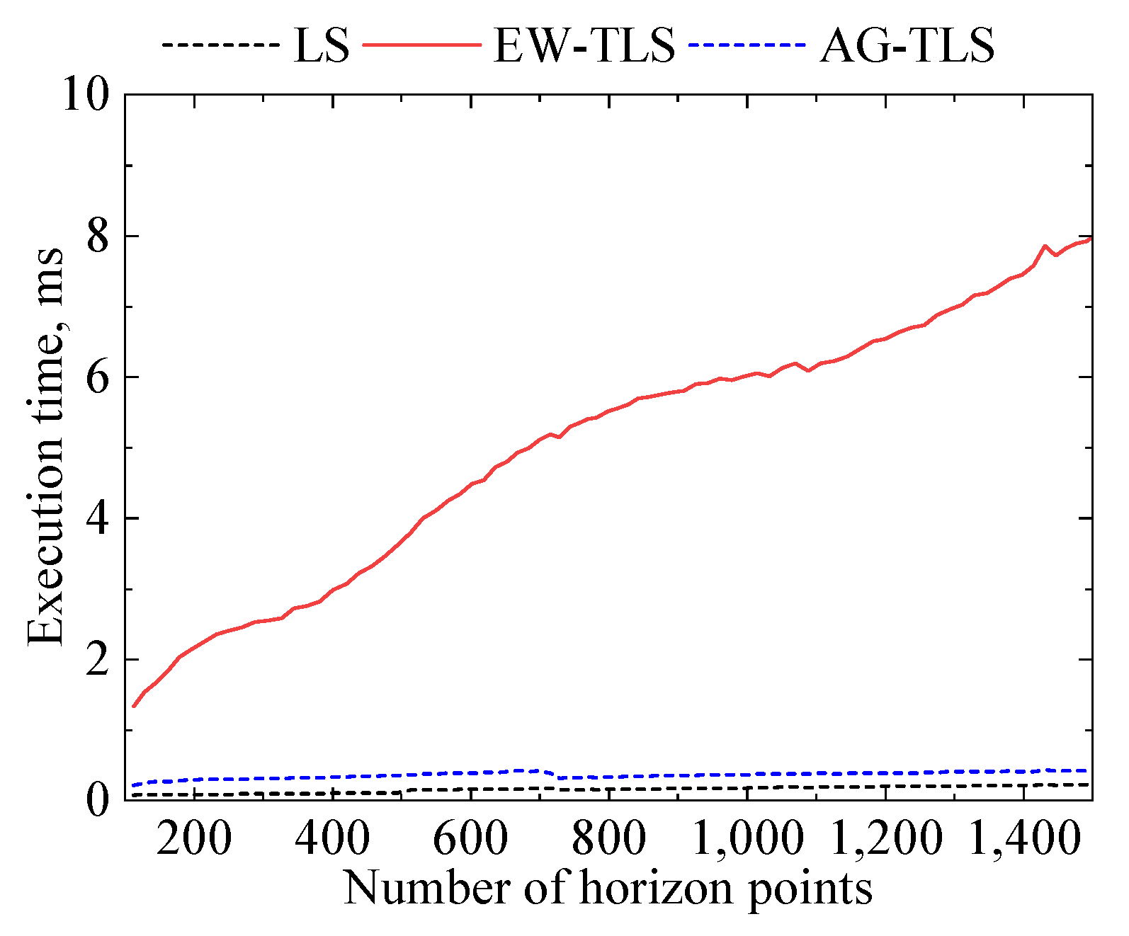
Additionally, it is necessary to evaluate the execution times of the algorithms. Simulations are running multiple times at different horizon arcs and the average value is obtained as execution times. They are running in a computer with an intel i7-10700 CPU and MATLAB 2022a. The execution times include only the navigation algorithms, not the time for image processing, etc. The number of horizon points gradually increases with the horizon arc, and the relationship between the number of horizon points and execution time is shown in Figure 7. It can be seen that the number of measurement points dominates the execution time of the algorithms. The execution time of the EW-TLS algorithm increases from 1.3 to 8.1 ms with the increase of horizon points. Most execution time of the EW-TLS algorithm is consumed during the iterations, and a small portion is used to calculate the covariance of each measurement. The execution time of the LS algorithm never exceeds 0.23 ms, while the execution time of the AG-TLS algorithm never exceeds 0.43 ms, and such extra computation consumption is often acceptable. Compared with the EW-TLS algorithm, the AG-TLS algorithm brings a huge speed improvement with a slight loss of precision, which is very suitable for onboard applications with limited computing resources.
4.3. Opnav Performance in a Highly Elliptical Orbit
To fully evaluate the performance of the short-arc horizon-based OPNAV, a navigation scenario in a highly elliptical orbit is tested. The scientific exploration orbit is usually a highly elliptical orbit to meet the requirements of communication and observation at the same time. Elements of the orbit around Mars are listed in Table 2. The test starts from the epoch 1 January 2022 07:49:00 (UTCG). In the frame P, the spacecraft’s initial position is (1.3212 , 2.4107 , −2.4834 ) km, and its initial velocity is (1.0999, 2.6389, 3.2311) km/s. The test covers 500 min, with perigee at the 0 and 470th minutes and the apogee at the 236th minute. The sampling interval for OPNAV is one minute. The parameters of the navigation camera are the same as those introduced earlier. The optical axis of the navigation camera is always aligned with the edge of Mars during the simulation, and the Mars horizon is on the diagonal of the image plane to ensure the best navigation performance. The influence of lighting conditions is not considered here to show the ideal situation, which may also be excluded by using an infrared camera, and the visible limb portion is always the entire one fitting within the camera’s FOV. The actual number of valid horizon points is always between 1700 and 1950. A total of 5000 sets of independent simulations are performed for each position, and the results shown are average values. Errors of OPNAV are presented in the camera frame C.
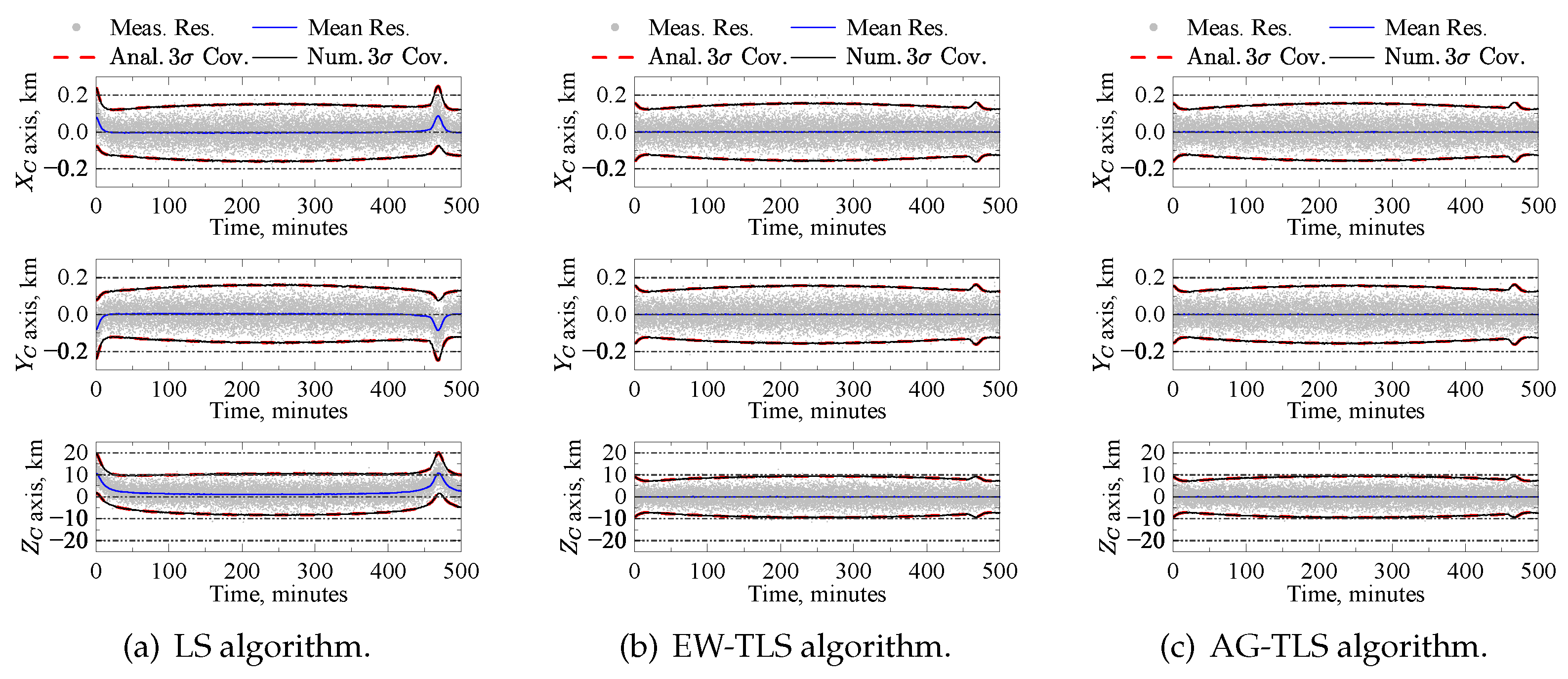
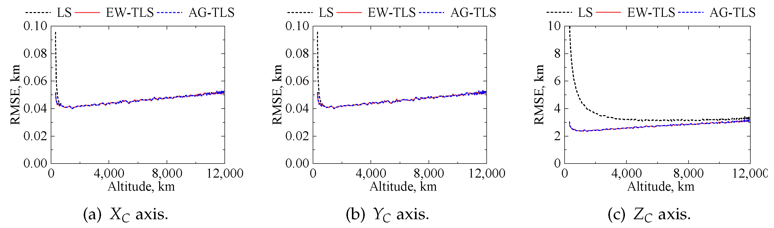
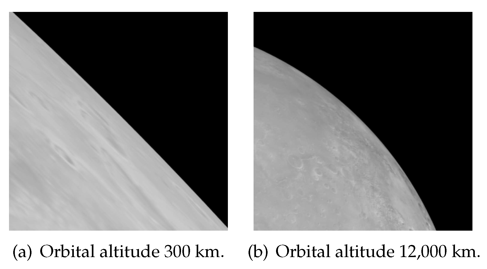
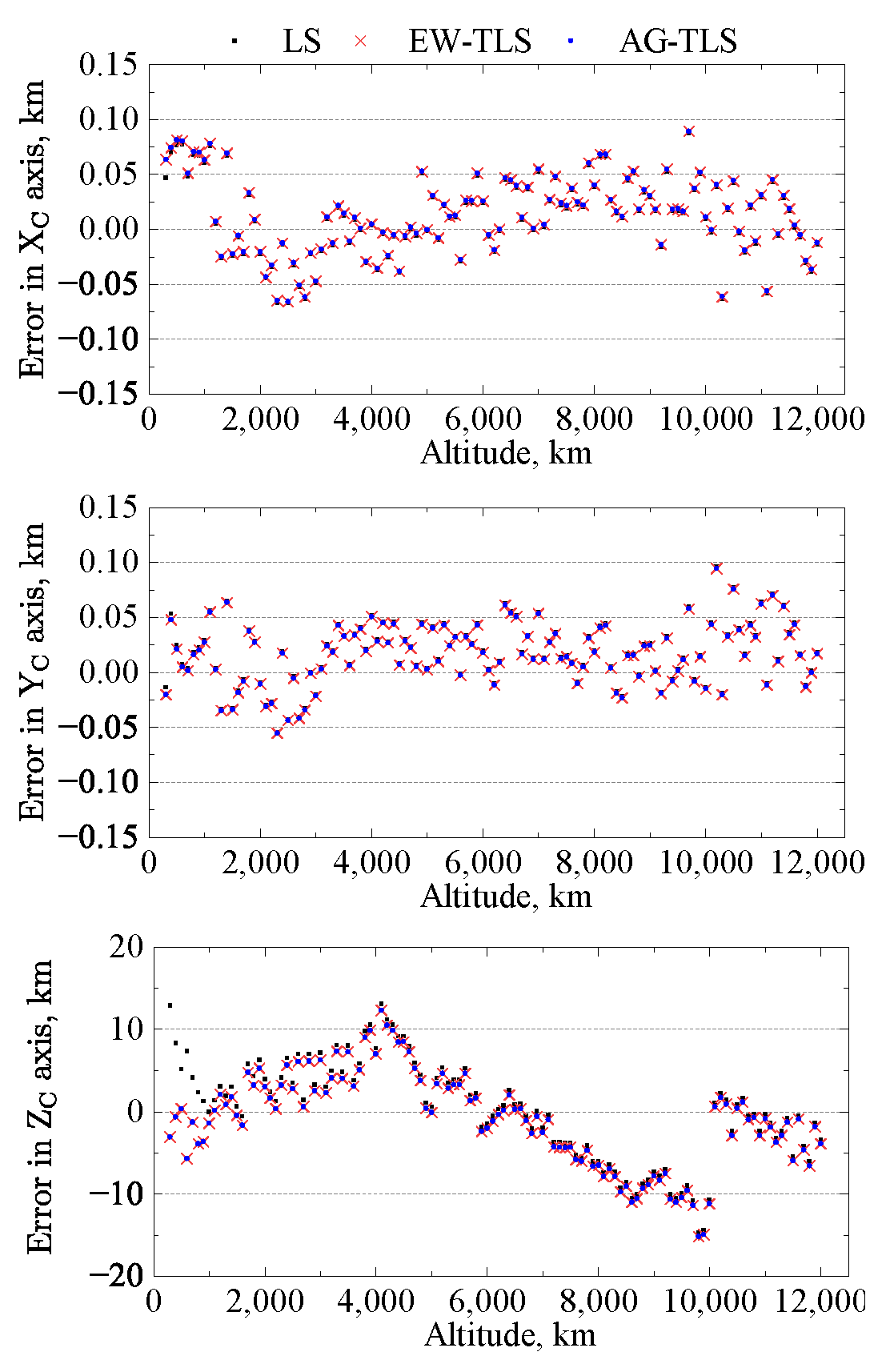
The Monte Carlo results of the LS algorithm, EW-TLS algorithm, and AG-TLS algorithm are shown in Figure 8. Gray points represent measurement residuals of Monte Carlo simulations, the blue solid line represents mean residuals of simulations, the red dash line represents 3 bounds of analytic covariance, and the black solid line represents 3 bounds of numeric covariance from simulations. Note that the covariance in Figure 8 is superimposed on the mean residuals. The three algorithms’ performances with the change in orbital altitude during the simulation are shown in Figure 9. The orbital altitude is raised from 300 to 12,000 km from perigee to apogee. The visible horizon arc length in the image plane gradually increases from 2 to 18 degrees as the orbital altitude is increased while, at the same time, the accuracy of each edge point gradually decreases. The horizon arc length and the edge point accuracy both affect the navigation accuracy and have opposite effects.
As shown in Figure 8b,c and Figure 9, there is a significant improvement in navigation accuracy with the increase of orbital altitude in the vicinity of the perigee. This shows that the increase in horizon arc length plays a dominant role in navigation accuracy at a low altitude. The navigation accuracy slowly decreases as the orbit altitude is further increased, which indicates that the decrease in the edge point accuracy at this time will affect the navigation accuracy to a greater extent. The STD of the navigation error ranges from 0.040 to 0.054 km in the and axes and from 2.374 to 3.188 km in the axis. The phase angle of the spacecraft does not show much effect in our simulation, which should be related to the small oblateness of Mars. As seen in Figure 8a and Figure 9, the LS algorithm shows a significant mean residual in the navigation results for all three axes at low orbital altitudes. The mean residuals of all three axes gradually decreases as the orbital altitude is further increased, and the influence in the and axes can be neglected. However, a certain mean residual has been maintained in the axis, and even at the apogee, there is still a mean residual of 1.16 km. While the mean residuals appear to be concentrated primarily along the axis, it is important to note that the impact of residuals becomes more intricate when analyzed within the planetary frame. The axis, which corresponds to the camera’s optical axis, is aligned with the edge of Mars. The attitude of the camera within the planetary frame varies as the spacecraft’s position changes. Consequently, the direction of the mean residuals will also be variable within the planetary frame. This means that the effect of the mean residuals should not be overlooked. On the contrary, the EW-TLS algorithm and AG-TLS algorithm both showed a better performance with near-zero mean residuals in different orbital altitudes. In general, the short-arc horizon-based OPNAV exhibits good accuracy throughout the entire orbital period, and it provides unbiased position estimation with the help of the TLS estimation.
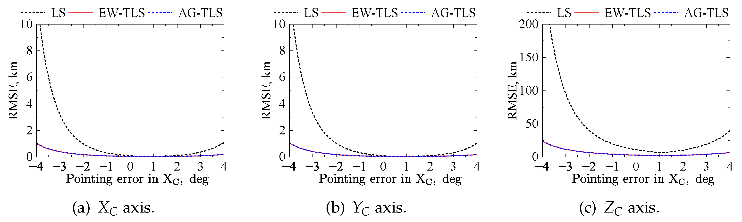
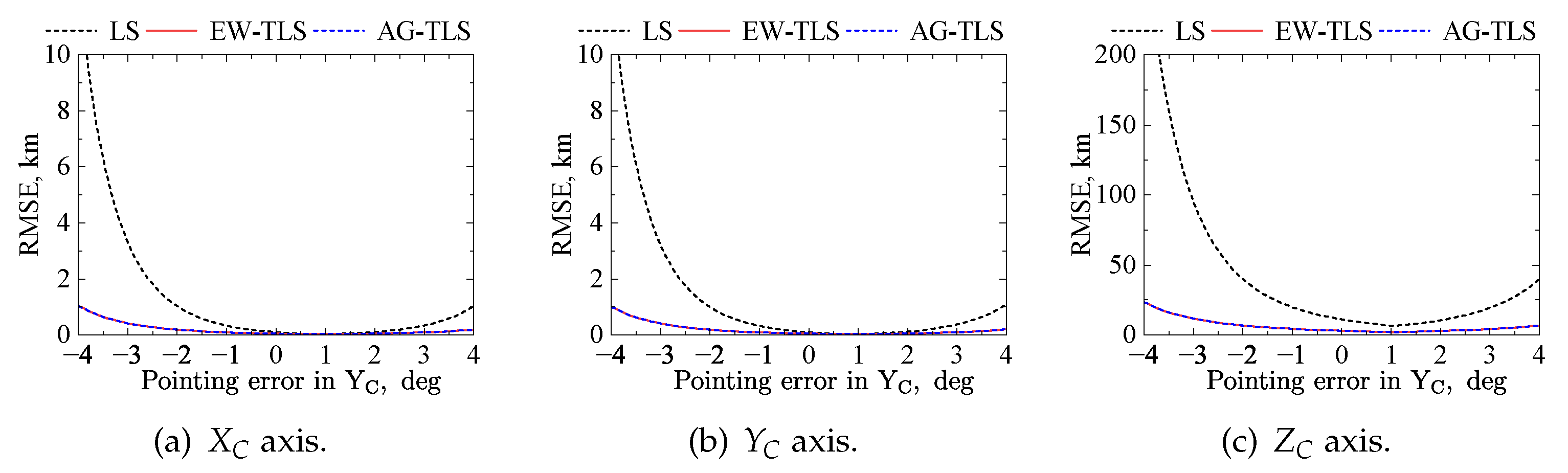
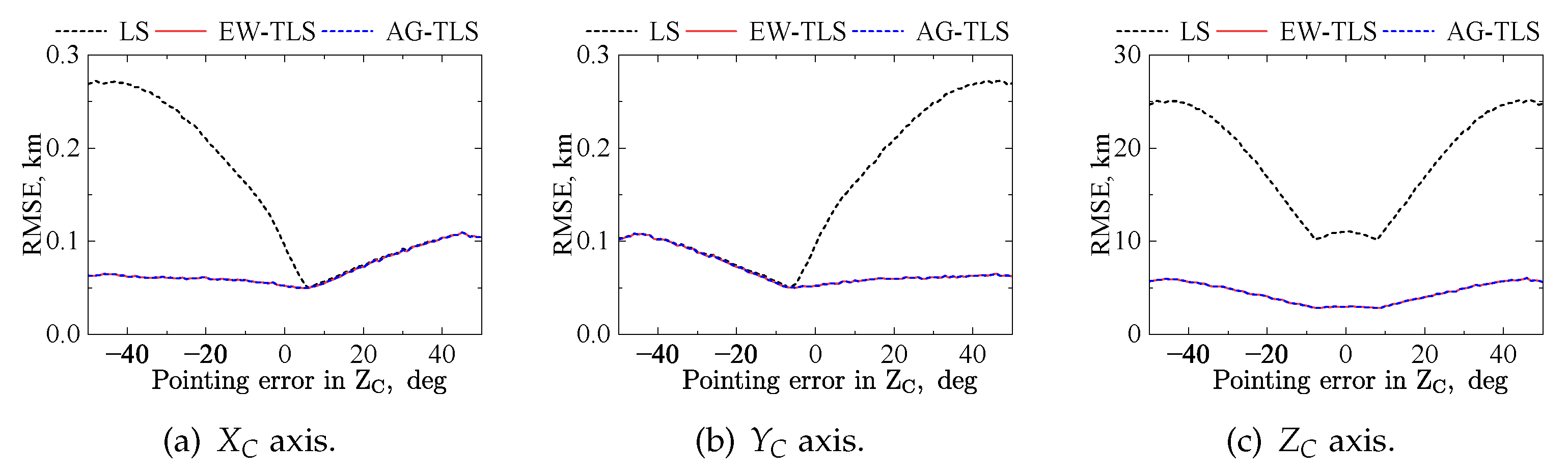
In addition to orbital altitude, the performance of short-arc horizon-based OPNAV is affected by pointing errors. Ideally, the optical axis of the navigation camera should point to Mars’ horizon, and the horizon should remain on the diagonal of the image plane to ensure the best navigation performance, while it is difficult to achieve such precise pointing in practice. Taking the perigee as an example scenario, the performance of horizon-based OPNAV with different pointing errors on the , , and axes of the navigation camera are shown in Figure 10, Figure 11, and Figure 12, respectively.
As the pointing error increases, the horizon arc taken by the navigation camera becomes shorter and the OPNAV performance gradually decreases. The performance degradation of the LS algorithm is particularly significant compared to the EW-TLS algorithm and AG-TLS algorithm. When the pointing error on or axis is -4 degrees, the LS algorithm’s positioning accuracy is worse than 10 km for both and axes and 200km for axis, while the EW-TLS and AG-TLS algorithms are better than 1 km for both and axes and better than 25 km for axis. With the pointing error around the axis, the horizon shifts from the diagonal of the image plane to the horizontal or vertical direction. For the EW-TLS and AG-TLS algorithms, the positioning accuracy of and axes decreases from 0.054 km to the worst, 0.108 km, and the positioning accuracy of axis decreases from 3.188 km to the worst, 6.000 km. Meanwhile, for the LS algorithm, the positioning accuracy of and axes ranges from 0.050 to 0.272 km, and the positioning accuracy of the axis ranges from 10.214 to 25.052 km. The pointing error in the axis has less impact on the optical navigation performance than the other two axes because the reduction of the horizon arc is smaller.
Pointing errors lead to the degradation of horizon-based OPNAV performance, and the EW-TLS algorithm and AG-TLS algorithm demonstrate a higher tolerance for pointing errors. The huge performance gap between the LS algorithm and TLS algorithms reveals the necessity of TLS estimation. Higher requirements should be placed in the pointing accuracy on and axes than the axis in the horizon-based OPNAV.
4.4. OPNAV Performance with Synthetic Images
To further validate the algorithm, the navigation performance after image processing is tested. Blender [42], an open source 3D computer graphics software program, is used for the synthesis of navigation images. Blender’s realism and convenience have made it popular in the field of OPNAV [43,44]. The specific steps of image synthesis and processing are as follows:
- (1)
- First, the basic simulation environment is built in Blender, including building Mars using its parameters and surface textures [45], setting up the navigation camera, and adding a light source to model the Sun. The parameters of the navigation camera are consistent with the previous section.
- (2)
- Next, automated rendering is implemented using the Python interface provided by Blender. Specifically, Python scripts are used to set the position and attitude of the sun and camera for each simulation scene, and the cycles engine is used to render photorealistic images. The camera is always pointed with its back to the Sun and toward the horizon of Mars to achieve good imaging.
- (3)
- Finally, MATLAB is used for image processing of rendered images. The images are convoluted by a Gaussian kernel with an STD of 1.5 pixels to simulate the effect of defocusing, then the algorithm proposed in [13] is employed to achieve subpixel edge localization.
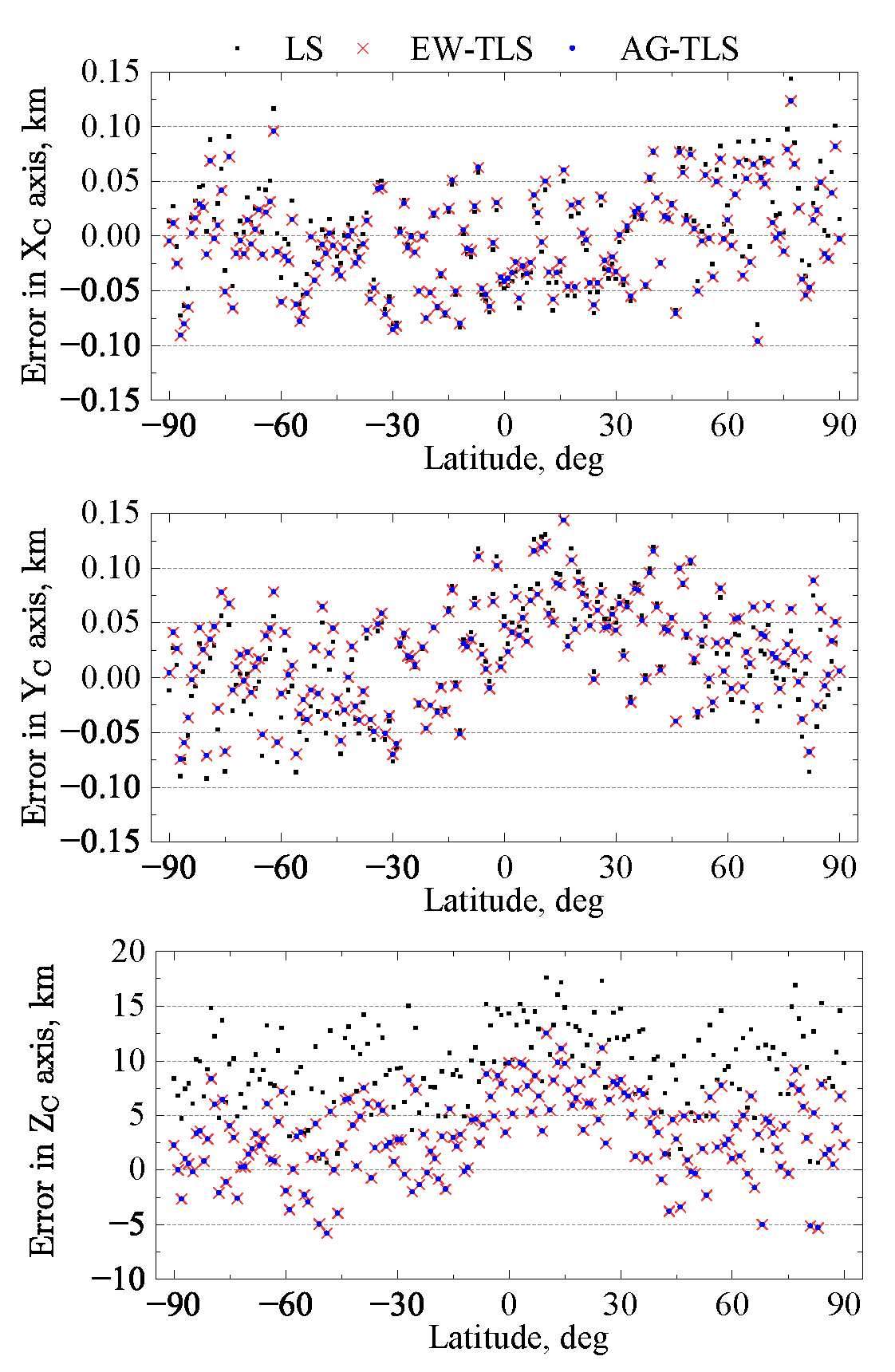
The example synthetic images for OPNAV around Mars are shown in Figure 13. It can be seen that as the orbit altitude decreases, the horizon no longer bends and gradually becomes straighter. OPNAV performance with synthetic images under different altitudes is shown in Figure 14. Due to the small number of simulations, the performance gap between the LS algorithm, EW-TLS algorithm, and AG-TLS algorithm is not significant. The navigation errors on the and axes are between ± 0.1 km, while the navigation error on the axis did not exceed ± 15 km. OPNAV performance with synthetic images at an orbital altitude of 300 km under different latitudes is shown in Figure 15. The navigation performance of the three algorithms seems to be similar on the and axes. However, there is a noticeable difference in their performance on the axis. The RMSE on the axis of the LS algorithm is 10.2 km, while the RMSE on the axis of the EW-TLS and AG-TLS algorithms are both 5.0 km. It can be seen that the LS algorithm showed certain mean residuals, which are well eliminated by both the EW-TLS algorithm and the AG-TLS algorithm. The performance of the proposed algorithms with synthetic images is not as good as in numerical simulation due to the limitation of simulation accuracy and edge positioning accuracy. However, the proposed algorithms can still bring considerable improvement to the performance of horizon-based OPNAV under a short-arc horizon scenario compared with the traditional algorithm.
5. Conclusions
To improve the performance of horizon-based OPNAV based on a short-arc horizon, a simplified measurement covariance model is proposed by further analyzing the propagation of measurement errors. Then, an unbiased solution with EW-TLS estimation is given by considering every element’s covariance of measurement equations. To further simplify this problem, an AG-TLS algorithm is proposed, which achieves a non-iterative solution by using the covariance of any one measurement as an approximation of all measurement covariances. Covariance analysis demonstrates that the covariances of the traditional Christian–Robinson algorithm with ordinary LS estimation and proposed algorithms are identical, and the difference between them lies in the possible estimation bias.
The numerical simulations under different horizon arc lengths show that when the horizon arc length is sufficiently long, both the traditional algorithm and the proposed algorithms achieve near-zero mean residual with consistent accuracy. With the shortening of the horizon arc length, the traditional algorithm will introduce a large mean residual that may even be larger than the STD, while the proposed algorithms both showed impressive advantages of near-zero mean residuals in the short-arc horizon scenario. Compared with the EW-TLS algorithm, the AG-TLS algorithm trades a negligible accuracy loss for a huge reduction in execution time and achieves a computing speed comparable to the traditional algorithm. Thus, the AG-TLS algorithm is very suitable for onboard applications with limited computing resources. Furthermore, as verified by the simulated navigation scenario with a highly elliptical orbit around Mars, a short-arc horizon can provide reliable position estimates for deep space exploration missions. Synthetic images with image processing further validate the effectiveness of the OPNAV method. The proposed algorithms extend the applicability of the horizon-based OPNAV method.
Author Contributions
Conceptualization, H.D. and H.W.; Methodology, H.D.; Software, H.D.; Validation, Y.L. and H.W.; Formal Analysis, H.D.; Resources, Z.J.; Draft Preparation, H.D. and H.W.; Writing—Review and Editing, Y.L. and Z.J.; Visualization, H.D.; Supervision, Z.J.; Project administration, Z.J.; Funding Acquisition, Z.J. All authors have read and agreed to the published version of the manuscript.
Funding
This research received no external funding.
Institutional Review Board Statement
Not applicable.
Informed Consent Statement
Not applicable.
Data Availability Statement
Not applicable.
Conflicts of Interest
The authors declare no conflict of interest.
References
- Huang, X.; Li, M.; Wang, X.; Hu, J.; Zhao, Y.; Guo, M.; Xu, C.; Liu, W.; Wang, Y.; Hao, C.; et al. The Tianwen-1 guidance, navigation, and control for Mars entry, descent, and landing. Space Sci. Technol. 2021, 2021, 13. [Google Scholar] [CrossRef]
- Williford, K.H.; Farley, K.A.; Stack, K.M.; Allwood, A.C.; Beaty, D.; Beegle, L.W.; Bhartia, R.; Brown, A.J.; de la Torre Juarez, M.; Hamran, S.E.; et al. The NASA Mars 2020 rover mission and the search for extraterrestrial life. In From habitability to life on Mars; Elsevier: Amsterdam, The Netherlands, 2018; pp. 275–308. [Google Scholar] [CrossRef]
- Gu, L.; Jiang, X.; Li, S.; Li, W. Optical/radio/pulsars integrated navigation for Mars orbiter. Adv. Space Res. 2019, 63, 512–525. [Google Scholar] [CrossRef]
- Bhaskaran, S. Autonomous Optical-Only Navigation for Deep Space Missions. In ASCEND 2020; American Institute of Aeronautics and Astronautics: Reston, VA, USA, 2020; p. 4139. [Google Scholar] [CrossRef]
- Hoag, D.G. The history of Apollo onboard guidance, navigation, and control. J. Guid. Control. Dyn. 1983, 6, 4–13. [Google Scholar] [CrossRef]
- Bhaskaran, S.; Desai, S.; Dumont, P.; Kennedy, B.; Null, G.; Owen, W., Jr.; Riedel, J.; Synnott, S.; Werner, R. Orbit Determination Performance Evaluation of the Deep Space 1 Autonomous Navigation System; JPL Open Repository: Pasadena, CA, USA, 1998; Available online: https://hdl.handle.net/2014/19040 (accessed on 6 April 2023).
- Foing, B.; Racca, G.; Marini, A.; Koschny, D.; Frew, D.; Grieger, B.; Camino-Ramos, O.; Josset, J.; Grande, M. SMART-1 technology, scientific results and heritage for future space missions. Planet. Space Sci. 2018, 151, 141–148. [Google Scholar] [CrossRef] [Green Version]
- Holt, G.N.; D’Souza, C.N.; Saley, D.W. Orion optical navigation progress toward exploration mission 1. In Proceedings of the 2018 Space Flight Mechanics Meeting, Kissimmee, FL, USA, 8–12 January 2018; p. 1978. [Google Scholar] [CrossRef] [Green Version]
- Bradley, N.; Olikara, Z.; Bhaskaran, S.; Young, B. Cislunar navigation accuracy using optical observations of natural and artificial targets. J. Spacecr. Rocket. 2020, 57, 777–792. [Google Scholar] [CrossRef]
- Hu, Y.; Bai, X.; Chen, L.; Yan, H. A new approach of orbit determination for LEO satellites based on optical tracking of GEO satellites. Aerosp. Sci. Technol. 2019, 84, 821–829. [Google Scholar] [CrossRef]
- Liebe, C.C. Accuracy performance of star trackers-a tutorial. IEEE Trans. Aerosp. Electron. Syst. 2002, 38, 587–599. [Google Scholar] [CrossRef]
- Christian, J.A. Optical navigation using planet’s centroid and apparent diameter in image. J. Guid. Control. Dyn. 2015, 38, 192–204. [Google Scholar] [CrossRef]
- Christian, J.A. Accurate planetary limb localization for image-based spacecraft navigation. J. Spacecr. Rocket. 2017, 54, 708–730. [Google Scholar] [CrossRef]
- Shang, L.; Chang, J.; Zhang, J.; Li, G. Precision analysis of autonomous orbit determination using star sensor for Beidou MEO satellite. Adv. Space Res. 2018, 61, 1975–1983. [Google Scholar] [CrossRef]
- Modenini, D. Attitude determination from ellipsoid observations: A modified orthogonal procrustes problem. J. Guid. Control. Dyn. 2018, 41, 2324–2326. [Google Scholar] [CrossRef]
- Christian, J.A. Autonomous initial orbit determination with optical observations of unknown planetary landmarks. J. Spacecr. Rocket. 2019, 56, 211–220. [Google Scholar] [CrossRef]
- Christian, J.A.; Derksen, H.; Watkins, R. Lunar crater identification in digital images. J. Astronaut. Sci. 2021, 68, 1056–1144. [Google Scholar] [CrossRef]
- McCarthy, L.K.; Adam, C.D.; Leonard, J.M.; Antresian, P.G.; Nelson, D.; Sahr, E.; Pelgrift, J.; Lessac-Chenen, E.J.; Geeraert, J.; Lauretta, D. OSIRIS-REx Landmark Optical Navigation Performance During Orbital and Close Proximity Operations at Asteroid Bennu. In Proceedings of the AIAA SCITECH 2022 Forum, Reston, VA, USA, 15 December 2022; p. 2520. [Google Scholar] [CrossRef]
- Silvestrini, S.; Piccinin, M.; Zanotti, G.; Brandonisio, A.; Bloise, I.; Feruglio, L.; Lunghi, P.; Lavagna, M.; Varile, M. Optical navigation for Lunar landing based on Convolutional Neural Network crater detector. Aerosp. Sci. Technol. 2022, 123, 107503. [Google Scholar] [CrossRef]
- Christian, J.A. Optical navigation using iterative horizon reprojection. J. Guid. Control. Dyn. 2016, 39, 1092–1103. [Google Scholar] [CrossRef]
- Teil, T.; Schaub, H.; Kubitschek, D. Centroid and Apparent Diameter Optical Navigation on Mars Orbit. J. Spacecr. Rocket. 2021, 58, 1107–1119. [Google Scholar] [CrossRef]
- Wang, H.; Wang, Z.y.; Wang, B.d.; Jin, Z.h.; Crassidis, J.L. Infrared Earth sensor with a large field of view for low-Earth-orbiting micro-satellites. Front. Inf. Technol. Electron. Eng. 2021, 22, 262–271. [Google Scholar] [CrossRef]
- Hu, J.; Yang, B.; Liu, F.; Zhu, Q.; Li, S. Optimization of short-arc ellipse fitting with prior information for planetary optical navigation. Acta Astronaut. 2021, 184, 119–127. [Google Scholar] [CrossRef]
- Christian, J.A.; Robinson, S.B. Noniterative horizon-based optical navigation by cholesky factorization. J. Guid. Control. Dyn. 2016, 39, 2757–2765. [Google Scholar] [CrossRef]
- Christian, J.A. A Tutorial on Horizon-Based Optical Navigation and Attitude Determination with Space Imaging Systems. IEEE Access 2021, 9, 19819–19853. [Google Scholar] [CrossRef]
- Franzese, V.; Di Lizia, P.; Topputo, F. Autonomous optical navigation for the lunar meteoroid impacts observer. J. Guid. Control. Dyn. 2019, 42, 1579–1586. [Google Scholar] [CrossRef]
- Crassidis, J.L.; Junkins, J.L. Optimal Estimation of Dynamic Systems; CRC Press: Boca Raton, FL, USA, 2012; Chapters 2 and 8. [Google Scholar]
- Crassidis, J.L.; Cheng, Y. Error-covariance analysis of the total least-squares problem. J. Guid. Control. Dyn. 2014, 37, 1053–1063. [Google Scholar] [CrossRef] [Green Version]
- Crassidis, J.L.; Cheng, Y. Maximum likelihood analysis of the total least squares problem with correlated errors. J. Guid. Control. Dyn. 2019, 42, 1204–1217. [Google Scholar] [CrossRef]
- Wang, B.; Li, J.; Liu, C.; Yu, J. Generalized Total Least Squares Prediction Algorithm for Universal 3D Similarity Transformation. Adv. Space Res. 2017, 59, 815–823. [Google Scholar] [CrossRef]
- Cheng, Y.; Crassidis, J.L. A Total Least-Squares Estimate for Attitude Determination. In Proceedings of the AIAA Scitech 2019 Forum, San Diego, CA, USA, 7–9 January 2019; American Institute of Aeronautics and Astronautics: Reston, VA, USA, 2019; p. 1176. [Google Scholar] [CrossRef] [Green Version]
- Almekkawy, M.; Carević, A.; Abdou, A.; He, J.; Lee, G.; Barlow, J. Regularization in ultrasound tomography using projection-based regularized total least squares. Inverse Probl. Sci. Eng. 2020, 28, 556–579. [Google Scholar] [CrossRef]
- Zhou, Z.; Rui, Y.; Cai, X.; Lu, J. Constrained total least squares method using TDOA measurements for jointly estimating acoustic emission source and wave velocity. Measurement 2021, 182, 109758. [Google Scholar] [CrossRef]
- Maleki, S.; Crassidis, J.L.; Cheng, Y.; Schmid, M. Total Least Squares for Optimal Pose Estimation. In Proceedings of the AIAA SCITECH 2022 Forum, San Diego, CA, USA, 3–7 January 2022; p. 1222. [Google Scholar] [CrossRef]
- Van Huffel, S.; Vandewalle, J. On the accuracy of total least squares and least squares techniques in the presence of errors on all data. Automatica 1989, 25, 765–769. [Google Scholar] [CrossRef]
- Schuermans, M.; Markovsky, I.; Wentzell, P.D.; Van Huffel, S. On the equivalence between total least squares and maximum likelihood PCA. Anal. Chim. Acta 2005, 544, 254–267. [Google Scholar] [CrossRef] [Green Version]
- Markovsky, I.; Van Huffel, S. Overview of Total Least-Squares Methods. Signal Process. 2007, 87, 2283–2302. [Google Scholar] [CrossRef] [Green Version]
- Forsyth, D.; Ponce, J. Computer Vision: A Modern Approach; Publishing House of Electronics Industry: Beijing, China, 2017; Chapters 1 and 2. [Google Scholar]
- Cheng, Y.; Crassidis, J.L.; Markley, F.L. Attitude estimation for large field-of-view sensors. J. Astronaut. Sci. 2006, 54, 433–448. [Google Scholar] [CrossRef] [Green Version]
- Shuster, M.D. Kalman filtering of spacecraft attitude and the QUEST model. J. Astronaut. Sci. 1990, 38, 377–393. [Google Scholar]
- Hikes, J.; Liounis, A.J.; Christian, J.A. Parametric covariance model for horizon-based optical navigation. J. Guid. Control. Dyn. 2017, 40, 170–178. [Google Scholar] [CrossRef]
- Community, B.O. Blender—A 3D Modelling and Rendering Package; Blender Foundation: Amsterdam, The Netherlands, 2022. [Google Scholar]
- Scorsoglio, A.; Furfaro, R.; Linares, R.; Gaudet, B. Image-Based Deep Reinforcement Learning for Autonomous Lunar Landing. In Proceedings of the AIAA Scitech 2020 Forum, Charlotte, NC, USA, 31 January–4 February 2021; American Institute of Aeronautics and Astronautics: Orlando, FL, USA, 2020. [Google Scholar] [CrossRef]
- Smith, K.W.; Anastas, N.; Olguin, A.; Fritz, M.; Sostaric, R.R.; Pedrotty, S.; Tse, T. Building Maps for Terrain Relative Navigation Using Blender: An Open Source Approach. In Proceedings of the AIAA Scitech 2022 Forum, San Diego, CA, USA, 3–7 January 2022; American Institute of Aeronautics and Astronautics: San Diego, CA, USA, 2022. [Google Scholar] [CrossRef]
- INOVE. Solar System Scope; 2017. Available online: https://www.solarsystemscope.com/textures/ (accessed on 6 April 2023).
Figure 1.
The geometry of the triaxial ellipsoid planet’s projection process.

Figure 2.
Simulated images of the horizon ellipse with different arc lengths.

Figure 3.
Monte Carlo results with a 15-degree arc horizon.

Figure 4.
Projected horizon ellipse in the image frame. For clarity’s sake, only 30 out of 5000 Monte Carlo sample histories are reported.
Figure 4.
Projected horizon ellipse in the image frame. For clarity’s sake, only 30 out of 5000 Monte Carlo sample histories are reported.

Figure 5.
RMSE with different horizon arc lengths.

Figure 6.
MSTDR with different horizon arc lengths.

Figure 7.
Execution time with different number of horizon points.

Figure 8.
Monte Carlo results of OPNAV performance. For clarity’s sake, only 30 out of 5000 Monte Carlo sample histories are reported (gray points).
Figure 8.
Monte Carlo results of OPNAV performance. For clarity’s sake, only 30 out of 5000 Monte Carlo sample histories are reported (gray points).

Figure 9.
OPNAV performance with different orbital altitude.

Figure 10.
OPNAV performance with different pointing error in the axis.

Figure 11.
OPNAV performance with different pointing error in the axis.

Figure 12.
OPNAV performance with different pointing error in the axis.

Figure 13.
Example synthetic images for OPNAV around Mars.

Figure 14.
OPNAV performance with synthetic images under different altitudes.

Figure 15.
OPNAV performance with synthetic images at an orbital altitude of 300 km under different latitudes.
Figure 15.
OPNAV performance with synthetic images at an orbital altitude of 300 km under different latitudes.


Table 1.
Monte Carlo results with a 15-degree arc horizon.
| Algorithm | Direction | Mean Residuals, km | STD, km | MSTDR | RMSE, km |
|---|---|---|---|---|---|
| axis | −296.82 | 95.25 | 311.63% | 311.73 | |
| LS | axis | −39.71 | 13.18 | 301.23% | 41.84 |
| axis | 5717.96 | 1834.61 | 311.67% | 6005.01 | |
| axis | 0.84 | 95.77 | 0.88% | 95.76 | |
| EW−TLS | axis | 0.04 | 13.22 | 0.34% | 13.21 |
| axis | −16.24 | 1845.42 | 0.88% | 1845.30 | |
| axis | −1.89 | 95.87 | 1.97% | 95.88 | |
| AG−TLS | axis | −0.37 | 13.23 | 2.78% | 13.24 |
| axis | 36.54 | 1847.53 | 1.97% | 1847.71 |
Table 2.
Elements of a highly elliptical orbit around Mars.
| Parameter | Value |
|---|---|
| Semi-major axis | 9500 km |
| Eccentricity | 0.61 |
| Inclination | 87 |
| Argument of perige | 320 |
| RAAN | 64 |
| True anomaly | 0 |
Disclaimer/Publisher’s Note: The statements, opinions and data contained in all publications are solely those of the individual author(s) and contributor(s) and not of MDPI and/or the editor(s). MDPI and/or the editor(s) disclaim responsibility for any injury to people or property resulting from any ideas, methods, instructions or products referred to in the content. |
© 2023 by the authors. Licensee MDPI, Basel, Switzerland. This article is an open access article distributed under the terms and conditions of the Creative Commons Attribution (CC BY) license (https://creativecommons.org/licenses/by/4.0/).
Share and Cite
MDPI and ACS Style
Deng, H.; Wang, H.; Liu, Y.; Jin, Z. Short-Arc Horizon-Based Optical Navigation by Total Least-Squares Estimation. Aerospace 2023, 10, 371. https://doi.org/10.3390/aerospace10040371
AMA Style
Deng H, Wang H, Liu Y, Jin Z. Short-Arc Horizon-Based Optical Navigation by Total Least-Squares Estimation. Aerospace. 2023; 10(4):371. https://doi.org/10.3390/aerospace10040371
Chicago/Turabian StyleDeng, Huajian, Hao Wang, Yang Liu, and Zhonghe Jin. 2023. "Short-Arc Horizon-Based Optical Navigation by Total Least-Squares Estimation" Aerospace 10, no. 4: 371. https://doi.org/10.3390/aerospace10040371
Note that from the first issue of 2016, this journal uses article numbers instead of page numbers. See further details here.