Air Traffic Complexity Evaluation with Hierarchical Graph Representation Learning

Abstract

Air traffic management (ATM) relies on the running condition of the air traffic control sector (ATCS), and assessing whether it is overloaded is crucial for efficiency and safety for the entire aviation industry. Previous approaches to evaluating air traffic complexity in a sector were mostly based on aircraft operational status and lacked comprehensiveness of characterization and were less adaptable in real situations. To settle these issues, a deep learning technique grounded on complex networks was proposed, employing the flight conflict network (FCN) to generate an air traffic situation graph (ATSG), with the air traffic control instruction (ATCOI) received by each aircraft included as an extra node attribute to increase the accuracy of the evaluation. A pooling method with a graph neural network (GNN) was used to analyze the graph-structured air traffic information and produce the sector complexity rank automatically. The model Hierarchical Graph Representing Learning (HGRL) was created to build comprehensive feature representations which involve two parts: graph structure coarsening and graph attribute learning. Structure coarsening reduced the feature map size by choosing an adaptive selection of nodes, while attribute coarsening selected key nodes in the graph-level representation. The experimental findings of a real dataset from the Chinese aviation industry reveal that our proposed model exceeds prior methods in its ability to extract critical information from an ATSG. Moreover, our work could be applied in the two main types of sectors and without extra factor calculations to determine the complexity of the airspace.

1. Introduction

ATM’s central component is air traffic service, which is made up of ATC service, flight intelligence service, and alert service, with ATC service acting as the foundation. ATC’s principal objective is to achieve effective discrimination and scientific guidance regarding the complexity of a particular air traffic situation (ATS). There is no agreed-upon definition of complexity [1], and this lack of consensus extends to the area of ATC as well, despite the widespread adoption of the notion of complexity and the growth of complexity science [2,3]. Air traffic complexity was initially established as a multidimensional concept comprising static sector features and dynamic traffic patterns, and it was underlined that air traffic complexity is indeed what drives the air traffic controller (ATCO) workload [4]. Moreover, complexity was defined as the degree of difficulty imposed on ATCOs under a particular traffic condition [5]. Despite the fact that the term “air traffic complexity” can be defined in a variety of ways, there is consensus in the field of ATC that rising air traffic complexity would eventually increase ATCO burden [6,7], so air traffic complexity is both positively and directly correlated with ATCO workload.

The crucial responsibility of an ATCO is to manage air traffic and maintain a safe, orderly, and productive ATM operation [8]. In the real civil aviation industry, a vast airspace is subdivided into a number of minor sectors that serve as the fundamental units of ATM. Typically, each sector is supervised by one ATCO, who is responsible for directing and supervising the air control and flight runway within his or her scope of responsibility, properly examining aircraft locations, resolving flight conflicts, etc. However, with the rapid growth of the aviation industry (although traffic volume decreased during the COVID-19 pandemic, it has since recovered significantly and will continue to grow in the future), the number of ATCO personnel has not kept pace, resulting in inconsistency of control resources and sector complexity. This has led to a chronically high workload for ATCOs and a greater possibility of making mistakes. It is well known that control errors can have catastrophic consequences, and risky incidents occur every year [9], such as aircraft flying too close to each other and a notorious one named the “Überlingen mid-air collision”. In this major accident, an ATCO was manning two consoles at once, and his workload was so heavy that he overlooked the potential conflict between two aircraft, leading to posting belated instructions that gave rise to the crash. If a machine or a model had replaced or assisted the controller in making a complexity assessment of the airspace before the accident and alerted the controller in a timely manner, the tragedy would not have occurred. Considering the growing complexity of ATS in the daily work of ATCOs, if a scientific and accurate method for real-time sector complexity assessment could be used to assist controllers, the potentiality of dangerous events would be massively reduced, ensuring the efficiency and safety of the entire civil aviation industry.

Real-time sector complexity assessment is a widely used decision aid in ATM [10,11,12,13,14]. If the need for such aid was not urgent in past flight scenarios with fewer aircrafts, efficient complexity assessment tools are critical and necessary in current airspace conditions due to increasingly complex air traffic flows. Consequently, the International Civil Aviation Organization (ICAO) offered the B3-NOPS module with the Aviation System Block Upgrade (ASBU) to propose an efficient ATM concept based on air traffic complexity assessment. Moreover, sector complexity is also a key factor in post-mortem analysis, with applications such as reconfiguration and optimization of airspace [10,15], efficacious supporting ground waiting strategy [16], and route planning [17].

Since Schmidt introduced the notion of air traffic complexity based on the “difficulty index” in 1976 [18], there has been a strong correlation between air traffic complexity and ATCO workload, sector capacity, etc. It has gradually become a research hotspot in the international ATC field, which is favored by ATC researchers and included as fundamental research in the U.S. Next Generation Air Transportation System (NextGen) construction plan [19] and the Single European Sky (SES) ATC research program [20]. The fundamental driver of the ATCO workload is the objective features of the air traffic flow. If there are more aircraft or if the route is more complex and changeable, the ATCO must exert more effort to deliver coordination instructions in a limited amount of time, resulting in an excessive workload during high-pressure missions. In response, if the ATCO is overburdened, he or she may experience mental fatigue and weakened work efficiency, leading to postponed issuance of instructions, lower-quality instructions, an inability to reply to pilot requests in a timely manner, and even wrong instructions. In actual ATC procedures, however, ineffective ATCOI results in delayed conflict resolution between aircraft and lagging aircraft attitude correction, which further complicates the airspace. Many studies have portrayed sector complexity from a subjective perspective by directly measuring ATCO physiological indicators or inviting them to fill out questionnaires [21,22]. Nevertheless, the majority of researchers have chosen to assess ATS based on real trajectory data or other objective factors and use ATS to infer controllers’ workload indirectly. The following is a thorough summary of the widely used approaches for evaluating air traffic complexity using air traffic flow.

Approaches for assessing the air traffic complexity could be grouped into two major categories and four subdivisions, with representative works for each type listed in

Table 1. Studies representative of evaluating air traffic complexity.

Category	Subcategory	Researcher	Evaluation Perspective	Evaluation Method	Result Presentation
Statistical Method	Single Viewpoint	Delahaye et al. [23,24].	Aircraft pair relative position	Geometric air traffic disorder metric	Geometrically complex coordinate system
		Delahaye et al. [25,26].	Lyapunov’s exponent-based trajectory disorder metric	Measure trajectory’s convergence and divergence	Lyapunov index magnitude
		Lee et al. [27,28,29].	Conflict resolution difficulty	Quantifying complexity as the required least control behavior	Complexity graph
		Prandini et al. [30,31].	Conflict risk assessment in sector regions	Conflict probability calculated from flight intention and status	Conflict possibility determines complexity
	Multi- viewpoint	Laudeman et al. [32].	Eight traffic parameters for Dynamic Density (DD) conceptualization	Linear regression methodology	Value of dynamic density
Machine learning method	Typical Indicator	Gianazza et al. [33].	Establish 28-indicators set and pick 6 factors	Backpropagation neural network (BPNN) model	Three-sector complexity level (CL) (low/normal/high)
		Xiao et al. [34].	Select 7 factors from 28-indicators set	BP-AdaBoost model
		Zhu et al. [35].	Utilize factor subset created by Xiao et al. [34].	Semi-supervised learning
		Cao et al. [36].	Twenty-eight-indicators set	Knowledge transfer methodology
		Li et al. [37].	Twenty-eight-indicators set	Deep unsupervised learning
	Feature Pattern Transformation	Xie et al. [38].	Design multichannel ATS image to replace feature set	Convolutional Neural Network (CNN) based model	Five-sector CL
		Tan et al. [39].	Seven graphical indicators computed from aircraft network diagram	Deep sparse autoencoder neural network model	Three-sector congestion level

. It is worth noting that the complexity evaluation we are discussing pertains to air traffic, not airspace complexity in a broader sense. In other words, airspace complexity is often determined by sector structure, waypoint composition, extreme meteorological circumstances, intense convective weather, military activity, etc. Current research on the evaluation of air traffic complexity has focused on the dynamic changes in aircraft as the primary research target.

Early methods of complexity evaluation fall within the scope of statistics, and researchers start from a single perspective and offer various single macroscopic indicators to describe the sector’s complexity. The first was aircraft density as proposed by the U.S. Enhanced Traffic Management System (ETMS) [40,41], followed by relative movement trends between aircraft pairs [23], trajectory disorder [26], difficulties in conflict resolution [27,28], and risk prediction [30,31], etc. Equally flexible is the output of these solutions, ranging from discrete distribution results to continuous numerical outcomes or direct exposition via graphical techniques. The commonality of the single-viewpoint group is that they are computationally simple and straightforward, but the complexity in the transportation domain is driven by a combination of numerous factors, and by extension in the ATC domain as well, where a single element cannot adequately gauge the whole traffic situation. To address this issue, the well-known DD concept was introduced [32], which involved picking multidimensional flight indicators, weighing the multiple metrics, and totaling to generate the DD score as a complexity measure. Unfortunately, the accuracy of complexity assessment results is constrained by the linear form, and the air traffic multi-attribute components exhibit highly nonlinear interconnections among themselves.

In response to the aforementioned flaws, a second main category of complexity assessment approaches has spawned a fair bit of research as machine learning has progressed year by year. During the evaluation, it is a prerequisite to build complexity feature-factor sets. The sets may consist of a great range of indicators, such as the total number of aircraft, the total number of climbing aircraft, the level of track disorder [42,43,44,45], etc. Among them, the most popular set is a collection of 28 metrics. Gianazza et al. [33] employed the PCA algorithm to extract six guided feature factors for feeding into BPNN, which then outputs the relevant sector complexity with three levels relying on the ATS-related input factors. On the basis of such a methodology and feature-factor set, the problem of assessing the complexity of air traffic has been converted into a CL classification task, which lies under the domain of supervised machine learning (ATS sample labels are directly calibrated by ATCOs). Since then, efforts have been focused on upgrading the network model and developing better ways for effectively selecting feature variables (such as AdaBoost [34]) to enhance the precision with which complexity is assessed. There are additional models that take advantage of small sample learning to cut back on the quantity of labeled samples required [35,36,37,46], but regrettably, the assessment accuracy has suffered. Labeled samples are labor- and knowledge-intensive, and they require a priori knowledge. The recent study converted air traffic situational data formats (a multichannel image [38] and flight situational network [39]) for automatic feature extraction instead of applying 28 traditional feature factors.

The efficacy of the aforementioned machine learning approaches has been clearly proven, but the existing models are unsatisfactory for the actual ATC process owing to the following shortcomings:

• Poor timeliness of complexity feature sets: The performance of machine learning models is directly correlated with the quality of feature sets, and the traditional 28-indicator set was proposed more than 10 years ago, which is incompatible with the fast-expanding ATM system and the continually evolving algorithmic frameworks. Furthermore, the potential complexity features may not be explored.
• Diversified sectors with distinct functions and structures, such as the approach control sector (SA) and the en-route control sector (SR), cannot be subjected to a fixed set of complexity-influencing variables. The common collection of feature factor sets disregards sector distinctions and cannot fully depict the ATS within a sector. In Appendix A, disparities between sectors are discussed.
• High cost of model manual front-loading: In terms of feature acquisition, construction using flight data is limited by challenges such as high computational cost, limited data sources, and a high demand for expertise. If the generation of feature sets is inadequate or there are computing faults, the model’s capability will be weakened.
• The feature pattern transformation technique requires improvement: Since the multi-channel picture approach has no need to calculate the complexity factor set, generating multi-channel images is pretty tough and may induce noise. The aviation network graph approach only considers the aircraft’s relative location while forming the graph, totally disregarding the flight trend’s effect on complexity, which hinders the accuracy of the obtained graph theory indicators (average node degree, average clustering coefficient, etc.).
• The feature selection perspective is unsatisfactory: Many of the features in the existing methods are extracted from the flight attributes, while CL and ATC are inextricably linked. The model will be less accurate and less interpretable if it lacks ATCO behavior elements.

According to the analysis of prior research, an HGRL-based model for sector complexity assessment was proposed by means of directly extracting features from a sector’s ATS without selecting complexity feature factors. To the best of our knowledge, this is the first time ATCOI has been introduced to the components of complexity feature sets in order to accomplish more accurate sector CL classification tasks. GNN-based models have achieved great performance in the field of ground traffic situational awareness. Inspired by this, we designed the graph convolutional neural network (GCN) [47] unit integrated with the hierarchical pooling module to retain hierarchical structure information in the graph. In order to more intuitively and thoroughly abstract air traffic, we replace the process of selecting complexity feature factors by constructing an ATSG, where the aircraft serves as the node and the connected edge conditions are designed from two perspectives: the aircraft’s position relationship and the flight trend. The experimental findings demonstrate the effectiveness of our proposed model across sectors with diverse functions and structures, with a noticeable increase in accuracy compared to the manual feature method. In addition, experiments confirm the superiority of the suggested network structure, proving that the structure learning module can extract graph structure features more efficiently.

As with the classic airspace complexity assessment methods listed in Table 1, our primary application scenario for proposing HGRL is to guide controllers in decision making. Meanwhile, we proposed an original approach of feature construction to replace the conventional metrics alongside improving the accuracy of the real-time assessment. Using our high-performance HGRL trained with a large amount of data, which generates the CL of the sector based on the aircraft flight situation in the airspace, provides a global view of the CL hints to controllers who are chronically overworked in the current actual control operations. For instance, the controller’s attention is frequently concentrated on the most conflict-prone local radar screen in the sector, while the ATCO ignores the upcoming conflicts in areas where he or she has not given sufficient attention. In this case, our approach helps ATCOs in implementing full situational monitoring of the flight situation and automatically outputting sector CL as contemporaneous feedback to controllers, thus enhancing ATCO efficiency, reducing ATCO workload, and confirming safe aircraft operations.

Additionally, the precise evaluation of HGRL’s complexity can prevent ATCO errors in the course of their actual working. The most common controller mistakes belong to the following three categories: mistakes, omissions, and forgetfulness. Firstly, it is probable for the controller to misjudge the overall air traffic condition, in which case HGRL can directly emit CLs to inform the controller and offer a measure criterion. Second, the ATCO may focus on a single aircraft or a small group of aircraft and ignore the impact of other aircraft on the entire air traffic situation, which HGRL can correct by synthesizing the correlation of all aircraft in the sector. Third, HGRL can provide controllers with a valid reference based on historical CLs if the ATCO forgets earlier chronological CLs because it can generate CLs continuously for a defined time period. If the evaluation of HGRL reveals that the CL tends to increase with time and retains at a high complexity level, it can be deduced that the controller is not deconflicted in a timely manner, indicating that he or she is always overburdened and prone to error. In the above scenario, HGRL can be utilized to inform the controller or assess whether airspace resources need to be redistributed promptly. In conclusion, HGRL is capable of providing excellent technical support to the ATC field.

The following is a brief summary of the significant contributions of this study.

• A general model for airspace sector complexity evaluation based on HGRL was developed in order to thoroughly and efficiently capture ATS characteristics and effectively identify sector CL automatically.
• The brand-new data structure, namely ATSG, was created in response to the airspace traffic scenario, which integrates aircraft operating attributes and proximity trends to appropriately depict ATS.
• From the perspective of ATCO–aircraft interaction, the complexity feature is expanded, and the unprecedented combination of aircraft operation and ATCOI as the affecting component of sector complexity enhances the accuracy of the model.
• An effective graph structure learning module utilizes node feature information and graph topology information to emphasize the relevance of key aircraft nodes for graph-level ATSG representation.
• Using realistic control scenarios and flight data, the approach is validated. Experiment results on SA and SR indicate that our method outperforms previous benchmarks and is applicable to both types of sectors with a certain extent of generalizability.

The remaining sections of the paper are arranged as follows: Section 2 describes the challenges faced during the evaluation of sector complexity and offers an overview of our HGRL approach. Our suggested HGRL procedure is detailed in Section 3. In Section 4, the model is verified with a real-world dataset. The experimental data processing methodologies, model assessment metrics, experimental settings, and experimental findings are also discussed. This study is summarized in Section 5 with a brief discussion on future work.

2. Problem Description and Method Overview

As stated in Section 1, the primary responsibility of ATCOs is to build situational awareness in their brains based on continuous dynamic trajectories and then apply land–air calls to issue coordinated instructions, which takes an enormous amount of attention. Therefore, the contemporary civil aviation environment seeks models that could be implemented in ATC processes that broadcast real-time airspace complexity. The ultimate realistic goal for recent machine learning-based complexity assessment models is to give real-time, high-precision CL feedback, and the proposed HGRL has the same practical application scenario.

In order to enhance the efficiency of HGRL assessment, ATCOI was first categorized and assigned to each aircraft as an extra feature. In each flight scenario, the particular instructions provided by ATCO may more accurately describe the air traffic operation situation, intuitively reflect the ATCO’s workload level, and then explain the relevant airspace’s complexity. To further elaborate, ATM is a multi-element coupled Human-in-the-Loop (HITL) system: the real-time ATS directly influences the workload of the ATCOs, while at the same time the working status and efficiency of the ATCOs in turn influence the present and future operational status of the aircraft. Thus, it makes practical sense to combine aircraft flight data with ATCOI to characterize sector situations. Between the time an ATCO issues an instruction to an aircraft and the time the pilot executes it, at least tens of seconds elapse. When conducting inter-sector aircraft handovers, this time lag can extend to several minutes, and the aircraft is so quick that a completely different ATS can be formed in a short amount of time. This also demonstrates that ATCOI forecasts the likely operational status of an aircraft in advance. Fusing the two types of data improves both the accuracy of HGRL and the safety of the flight. If air traffic complexity is assessed only on aircraft trajectory, the controller’s short-term prediction is ignored, and the assessment’s dimensionality is accordingly decreased.

Since the introduction of the BPNN-based [33] solution, the air traffic complexity evaluation problem has steadily evolved into a standard machine learning problem, which is purely a classification problem (characterized by complexity feature-factors and labeled by CL). We directly adopted the controller’s professional opinion when determining CL since this method provides a full evaluation of the airspace condition from the controller’s perspective. We did not employ objective evaluation indicators since there has never been a unified definition of airspace complexity classification, and because the prior rule-based complexity classification criteria were quite wrong. For instance, the CL was calibrated in accordance with the number of aircraft in the airspace [40]. Still, there are situations that cannot be precisely measured, such as when multiple aircraft in one sector are traveling at separate altitudes and there is no chance of interaction between them. The approach of defining CL based solely on the number of aircraft is therefore flawed. Rule-based approaches of CL calibration, such as this, lack the comprehensiveness of complexity representation; therefore the direct marking of CL by experienced ATCO is widely utilized in relevant studies [34,35,36,37,38,39] as well as in this paper.

The theory of complex networks is frequently employed in the transportation area [48,49]. Air traffic complexity is described using this theory and its topological properties are derived from the structure of connections between aircraft [50,51,52]. Inspired by this, we converted the air traffic scenario information acquired from the radar screen into a “graph snapshot” format and then extracted important information using the GNN technique, which is used to complete the sector complexity evaluation project. The structure of the new trajectory data format might include the proximity between aircraft as well as other crucial control characteristics. This solution faces two primary obstacles:

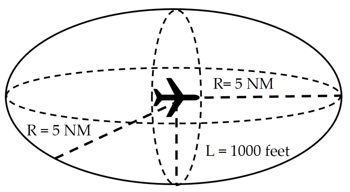
• Establish an ATSG capable of fully reflecting the comprehensive information of space location and the approaching trend between aircrafts. ATCO’s primary responsibility is to resolve conflicts, avoid possible conflicts, and minimize negative chain effects following the delivery of instructions. Therefore, in order to prevent the occurrence of conflict false alarms, which will increase the ATCOs’ workload, it is important to develop a flight network that can effectively detect the conflict connection in three-dimensional space and meet the actual flight safety boundary criteria.
• The assessment model for ATCS complexity must be able to describe a substantial amount of training data. Moreover, when employing GNN, we should save as much information as possible on the topology of ATSGs. The sector CL is mostly influenced by the correlation between aircraft pairs as opposed to the inherent information of individual nodes. In a nutshell, the final performance of the model depends heavily on its structure design. The degree of structural information retention must be considered, as well as the existence of noise information.

In light of the aforementioned difficulties, we suggested a novel framework for measuring the complexity of sectors using the well-designed HGRL strategy. Figure 1 depicts the overall structure of the assessment architecture, which consists of three procedures:

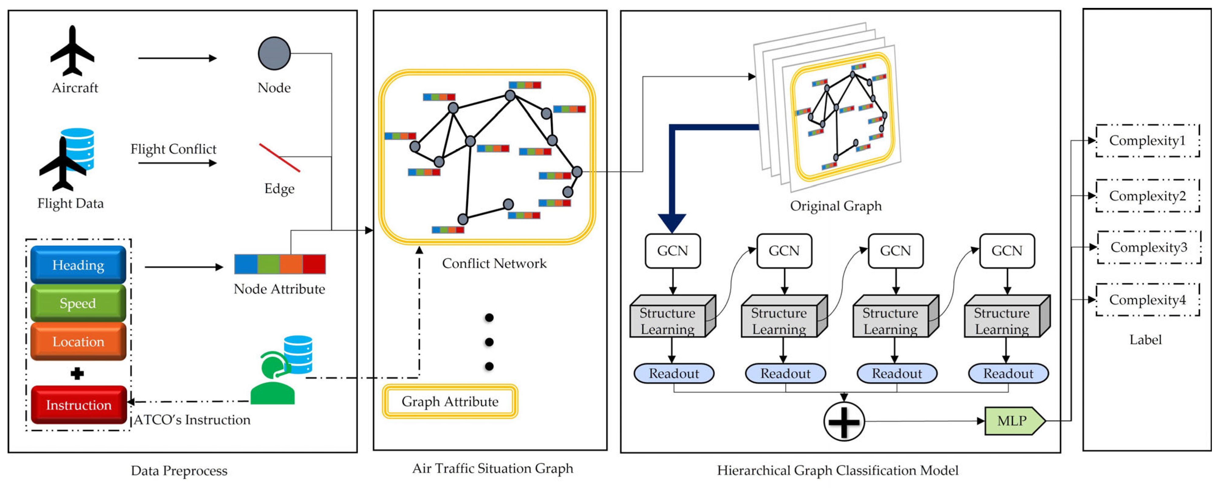
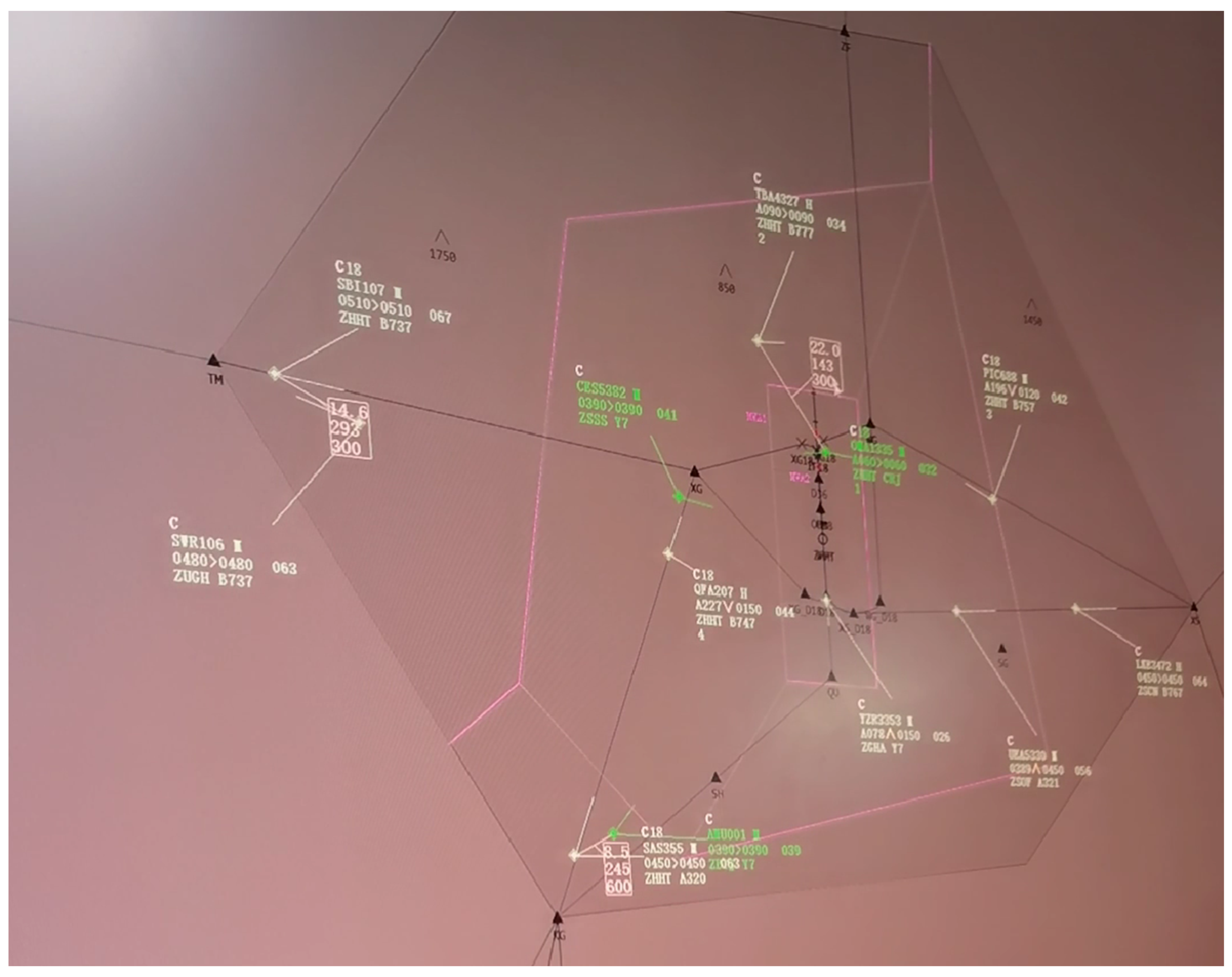
• Data Preprocess: Automatic Dependent Surveillance–Broadcast (ADS-B) transmission equipment was used to gather the sector’s dynamic data, which covered the primary trajectory information and a richness of aircraft operation data. Before converting air traffic scenarios into ATSGs, we collected the relevant instructions from ATCOs and requested that they rank and label their complexity.
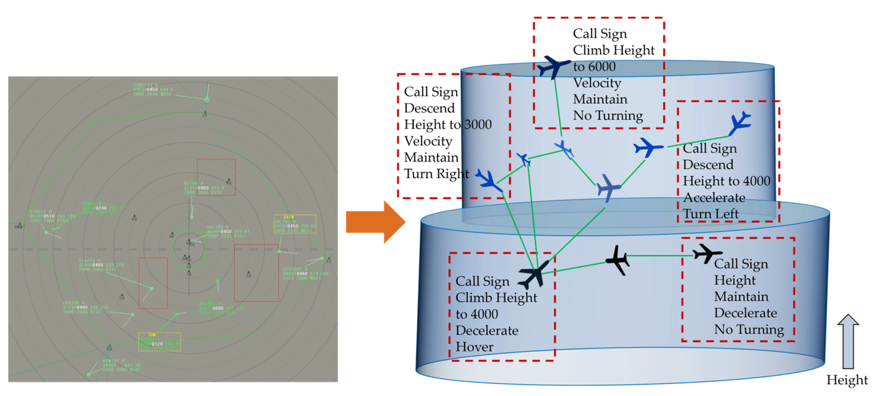
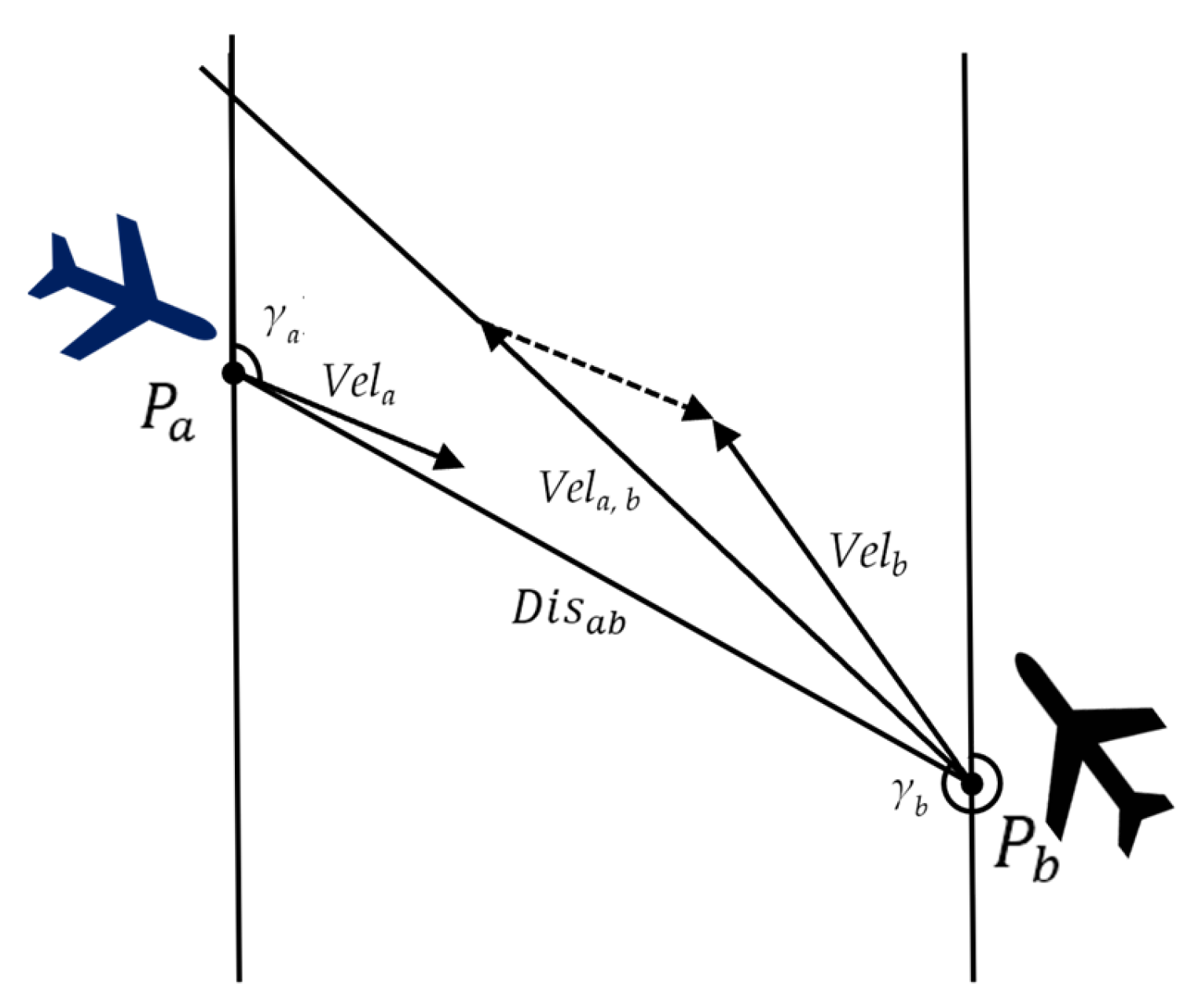
• Flight Conflict Network Construction: In order to further describe the current state of the airspace, the next step was to construct an FCN that was based on actual and potential conflict links between aircraft. In the majority of flight state networks, the interdependency between aircraft is merely connected to the conventional safety distance. In reality, the relative speed between two aircraft is also a crucial criterion for assessing the conflict scenario. Therefore, relative speed is a factor that we have considered while constructing a flight state network.
• Hierarchical Graph Classification Model: The FCN constructed in the unit of one minute was modeled as an ATSG, which comprises the node attribute and the entire graph attribute. Inputting enough ATSGs into the proposed hierarchical graph representation model (HGRM), which includes several graph convolutional layers, pooling layers, and multi-layer perceptron (MLP), will yield the output label data (sector CL).

3. Methodology

In this part of the paper, we are going to talk about the preparation of the targeted sector operation complexity assessment dataset, the extraction process and the applications of ATCOI throughout the entire process, the FCN, and the proposed HGRM.

3.1. Materials

Generally, our method falls under the category of supervised deep learning, which has high data requirements along with the creation of feature datasets and label datasets. A significant number of ATSGs (the generation of which required the assistance of trajectory data) were utilized as samples. The feature dataset matched the aircraft node characteristics in ATSGs (flight data concatenated the ATCOI received by each aircraft), and the label dataset corresponded to the graph attribute of ATSGs.

To fulfill the fundamental prerequisites of supervised machine learning, the foremost objective is to generate a large-scale dataset comprising CL annotations for aircraft operations. This dataset comprises two essential components: the complexity feature set and the complexity tag set. The feature set is obtained by computing multiple data sources, including airspace static structure data, ADS-B data, etc. The tag set is derived from the human labeling of specific air traffic scene samples by ATCOs. The airspace static structure data provide essential information, such as sector boundary latitude and longitude data, sector upper and lower altitude data, and so on, that is required for defining the regional location of the target sector and screening the traffic operational data.

• Complexity Feature Set: The ADS-B data used for this study are updated each second. However, because the operational complexity of the airspace does not vary significantly over short intervals, modeling the air traffic scenes per second directly would generate a large amount of sample data with similar complexity, resulting in data redundancy and a high computational burden. Therefore, we employed the common principle of the coarse granularity processing of trajectory data (in preparation for the next step in constructing the ATSG) by dividing time into 1-min intervals, as was employed in previous research [34,36,37,38,39,46]. In actuality, it is difficult to obtain ATCOs’ speech collection. To address this issue, real ADS-B data were inputted into the control simulator for realistic scenario restoration, and 3 senior ATCOs were invited to obtain command data, which were characterized according to the ATCOI classification principles discussed in the following section of the paper. Multiple instructions are frequently issued to the same aircraft within a 1-min interval, so we used the most recent ATCOI as the effective complexity feature rather than the previous ATCOI since the timeliness of the feature description cannot be guaranteed for the previous ATC situation.
• Complexity Tag Set: Present machine learning-based traffic complexity assessment research uses two primary labeling strategies: one is based on the actual split or merger state of the sector to reflect the complexity of sector operation [53], which can be obtained automatically from historical control data records, and the other is based on a manually collected CL, which is traditionally used as a 3-level label (low, medium, high) [34,36,37,46]. Although better results have been achieved in terms of assessment accuracy, this 3-level form provides limited information in actual control scenarios, making it challenging to provide decisionmakers with more detailed information as well as being an overly simplistic and crude approach. Due to the increase in existing traffic demand, the airspace sector frequently has abnormally high traffic complexity for the majority of the time. However, the traffic complexity does not typically reach the maximum level without exceeding the controller’s workload guarantee, so the optimal position for such a state of traffic complexity should be between medium and high. Consequently, a modest increase in CL level numbers may have a greater potential value in practical applications.

Our proposed method invites 3 experienced ATCOs with similar personal conditions to conduct a comprehensive CL assessment of historical air traffic scenarios. This is done by viewing ATC replay videos through the control mirror system, taking into account factors such as traffic volume, flight conflicts, control difficulty, and environment. The hierarchical assessment ATCOs are divided into 2 groups: the assessment group and the verification group. The assessment group consists of 2 ATCOs who perform CL assessment on all samples, while the verification group is responsible for verifying the ambiguous samples when the results of the assessment group are inconsistent. The evaluation time granularity is set to 1 min, and the CL is divided into 4 levels, which are described in detail in

Table 2. CL specification detail.

CL	ATC Difficulty	ATS Description
1	No need for intervention with flight. Ample spare capacity. Low workload.	Smooth air traffic. Sufficient flight interval. Orderly aircraft flight. Safe and efficient air traffic
2	Well-progressing ATC. All tasks under control. Normal workload.	Increased number of aircraft. No traffic congestion. Quickly fixed aircraft disturbance. Normal sector operation.
3	Increased ATCOI. Unable maintaining this level for very long. Saturated workload.	Minor sector congestion. Several affected aircrafts. With ATCO stepping a lot to keep sector working normally. Inefficient air transportation
4	Unfinished ATC tasks. No spare capacity. Excessive workload.	Widespread air traffic congestion. Increased chance of inter-aircraft conflict. Frequent flight delays. Overloaded airspace utilization.

.

During the actual evaluation process, ATCOs are required to perform a graded tagging process every minute for the corresponding situational scenarios. To ensure the quality of tagging, each ATCO works continuously for no more than 30 min during the tagging process. For instance, in Figure 2’s ZHHH SA, Wuhan flight information region (FIR), the ATCO needs to coordinate a total of 12 aircrafts and issue a total of 9 commands in a 1-min time period, which is denoted as CL-3 in our data set.

3.2. Air Traffiic Control Instruction Extraction

The most critical intuitive element of the controlling process is the number and content of ATCOI: timely and accurate ATCOI can effectively deconflict potential risks, while inefficient or even incorrect ATCOI can lead to undesirable knock-on effects, such as a potential conflict between aircraft being deconflicted when an ATCOI is issued as well as creating more aircraft conflicts, thereby increasing the overall complexity. Recent research on ATCOI has been focused on the domain of speech recognition [54,55,56,57,58], with minimal application to complexity assessment, so we unprecedentedly make a direct extraction of ATCOI to enrich the representation of ATS.

ATCOs offer instructions to aircraft crews based on the actual spatial–temporal environment of the operating sector and their own relevant job expertise, which mostly entails ground-to-air communication, route coordination and management, and warning alerts. To better comprehend the intricacies of air traffic control operations, it is necessary to classify and analyze the various types of orders used by air traffic controllers (ATCOs). As shown in

Table 3. Different control types of ATCOI.

ATCOI Type	ATCOI Content
Common ATC term	Maintain own separation and Visual Meteorological Condition (VMC) to (level)
Airport ATC term	Right (or left) turn approved
Approach ATC term	Expected approach time (time)
En-route ATC term	Maintain (level) while in controlled airspace
Coordination term between air traffic service units	(aircraft call sign) Not released until (time or significant point)
Radar term	Radar contact [position]
Automatic Dependent Surveillance (ADS) term	ADS
Term between ground crew and flight crew	Commencing pushback
Reduced Vertical Separation Minima (RVSM) term	Unable RVSM due [Turbulence]
Alert Term	(aircraft call sign) Terrain alert (suggested pilot action, if possible)

, the various ATCOI control types can be categorized into 10 groups. Each of these categories represents a different aspect of ATCO control and highlights the diverse range of responsibilities that ATCOs must handle in their daily work. By exploring these control types in depth, we may obtain a greater understanding of the challenges ATCOs encounter and how they manage complex air traffic scenarios.

These instructions are delivered to different and complex objects, making it impossible to directly classify them into a cohesive structure, as shown in Table 3. Since this study focuses primarily on the effect of the real-time flying condition in a given sector on complexity, the command-oriented objects are limited to the “ATCO-Pilot” range. Based on this, we abstract the radar screen facing the controller, as depicted in Figure 3, and the two-dimensional plane into a three-dimensional view for ease of comprehension. The cylinder denotes the altitude level at which the aircraft is located, the red dashed box indicates the instruction provided to an aircraft (if no command is given, the aircraft operates autonomously), and the green solid line indicates the possibility of spatial dependency between aircraft. Here is an example of an ATCOI: “CES123, Shanghai, radar identified, PIKAS11 departure, further climb and maintain 2400 m on QNH1012”; from this, we can derive the structure of commands that truly alter the flight attitude of an aircraft, comprising three major elements: altitude command, speed command, and heading command. By coarse-graining the ATCOI employed in our model in Figure 4, the aircraft receiving the command gains the attributes associated with the ATCOI, adding multidimensional features for the ATSG construction in the following step.

The particular contents of the category ATCOI are as described below: (a) Velocity Instruction: ATCO adjusts aircraft speed per flying stage. The ATCO will tell the crew to “decelerate” when the aircraft approaches runway speed in the approaching stage, command “accelerate/decelerate” during en-route flying, and send speed deployment orders for terminal conflict resolution. (b) Height Instruction: Flying altitude levels are defined by the fundamental flight regulations and vary per airspace. Thus, the height instruction should match the altitude level. Height-adjusted commands usually begin with “climb/descend/maintain”. (c) Heading Instruction: The heading of an aircraft is the angle from the northern end of the reference line taken clockwise to the projection of the aircraft’s longitudinal axis on the horizontal aircraft, 0–359°. The ATC gives orders formatted as “turn left/turn right”.

3.3. Flight Conflict Network Construction

According to the accepted definition, groups of vertices and edges make up the essential components of a graph. In the suggested method, vertices represented the collection of aircraft in a sector at a given time step. The distance that existed between 2 aircraft served as the criterion for determining these links. In other words, a continuous edge is created when the distance between 2 aircraft is smaller than some predetermined minimum.

The precise value of the preset minimum will be derived from two considerations: the spatial proximity interaction and the velocity proximity interaction of the aircraft pair, respectively. Maintaining a minimal safety separation requirement between aircraft is used to compute the spatial proximity relationship. If the relative location of two aircraft is close but does not exceed the minimum separation distance, the velocity proximity relation is launched. The velocity proximity relation is utilized to estimate the convergence/divergence conditions of aircraft pairs and to compute the approximation effect between aircraft. This twofold judgment will result in a more accurate adjacency matrix for the ATSG, ensuring that neither the present conflict situation nor the impending conflict situation between aircraft is overlooked. Moreover, this way of construction does not deliver duplicated edges, which will render the description of aircraft dependencies ambiguous. This strategy allowed us to simplify the monitoring situation’s intricacy while still obtaining essential data concerning airplane proximity.

For the spatial proximity, the ellipsoidal flight protection zone for aircraft was established according to the standard interval distance (5 NM (denoted as $R$) horizontally and 1000 feet (denoted as $L$) vertically [59]), the one that is most often employed, as depicted in Figure 5.

Suppose the ellipsoid distance between aircraft $a$ and $b$ at a given moment is $E_{a,b}$; ${(x}_a{, y}_a{, z}_a)$ and ${(x}_b{, y}_b{, z}_b)$ are the coordinates of $a$ and $b$:

$$E_{a ,b}=\sqrt{\left(\frac{{\Delta x}_{ a,b}^2}{R^2}+\frac{{\Delta y}_{ a,b}^2}{R^2}+\frac{{\Delta z}_{ a,b}^2}{L^2}\right)}$$

(1)

We determined the position relationship and whether there was an edge connection by computing the result of $E_{a, b}$, which results in 3 cases: (a) if $E_{a, b} > \sqrt{3}$, then $a$ is outside the protected zone of $b$, no conflict exists, and an edge will not be built between them; (b) if $E_{a, b} \le 1$, then $a$ is inside the protected zone of $b$, $a$ and $b$ are in flight conflict, edge constructed; and (c) if ${1 < E}_{a, b} < \sqrt{3}$, $a$ may enter the protected area of $b$ or may be outside the protected area of $b$ but extremely near to the boundary.

For an uncertain case, such as (c) above, the next step is to calculate the velocity proximity between aircraft to determine if edges exist between aircraft nodes. The proximity effect of an aircraft pair can also be understood as the convergence/non-convergence posture of the aircraft, and the aircraft position and velocity attributes are the most essential elements to analyze this effect. The position and velocity of the aircraft are denoted by Pos and Vel, respectively. The relative distance and relative velocity between $a$ and $b$ are denoted by ${Dis}_{a, b}$ and ${Vel}_{a, b}$, respectively, as shown in Figure 6. ${Dis}_{a, b}$ and ${Vel}_{a, b}$ are denoted, respectively, as Equations (2) and (3).

$$\begin{gathered} {Dis}_{\mathrm{ab}} {=Pos}_a-{ Pos}_b=\left(x_a-{ x}_b,{ y}_a-{ y}_b\right) \\ \parallel { Dis}_{\mathrm{ab}} \parallel =\sqrt{{{(x}_a-{ x}_b)}^2{+( y}_a-{ y}_b{)}^2} \end{gathered}$$

(2)

$${Vel}_{a, b}= \left({Vel}_{a}sin({\gamma }_a)-{Vel}_{b}sin({\gamma }_b),{Vel}_{a}cos({\gamma }_a)-{Vel}_{b}cos({\gamma }_b)\right)$$

(3)

The rate of proximity effect ${Pro}_{a, b}$ can be expressed as the component of the relative velocity on the line between the two aircraft:

$${Pro}_{a, b}= \parallel {Vel}_{a, b}\parallel cos(\angle {(Vel}_{a, b}{, Dis}_{a, b}\left)\right)=\parallel {Vel}_{a, b}\parallel \frac{\left({Vel}_{a, b} \cdot {Dis}_{a, b}\right)}{\parallel {Vel}_{a, b}\parallel \parallel Di{s}_{ab} \parallel } =\frac{\left({Vel}_{a, b} \cdot {Dis}_{a, b}\right)}{ \parallel Di{s}_{ab} \parallel }$$

(4)

From Equation (4), we can see that when ${Pos}_{a, b} > 0$, the 2 aircraft are in dispersion, and an edge between aircraft nodes in the ATSG will not be built. However, when ${Pos}_{a, b} < 0$, the aircraft pair is in convergence, this will increase the possibility of a more complex situation in the near future, with a link between aircraft being established consequently.

3.4. Hierarchical Graph Classification Model

3.4.1. ATSG Representation

After creating the FCN, let $G=(V, E, A, X)$ represent each ATSG, in which $N=\left|V\right|$ denotes nodes and edges are indicated by $\left|E\right|$. $A\in {\{0,1\}}^{N\times N}$ is an adjacency matrix defined by the connection principal in Section 3.3 and $X\in R^{N\times f}$ denotes the node feature matrix. $f$ symbolizes the dimension of node attributes, including heading, speed, location, and instruction information. Given a collection of CL-labeled ATSGs: $G_{CL}=\left\{\left(G_1{,CL}_1\right),\left(G_2{,CL}_2\right)), \dots \right\}$, where ${CL}_i\in \mathcal{C}\mathcal{L}$ is the complexity label attached with $G_i\in \mathcal{G}$; obtaining a mapping $m:\mathcal{G}\to \mathcal{C}\mathcal{L}$ is what graph classification aims to do. Using GNN, we wanted to accurately identify the unknown CL of $G_{CL}$.

3.4.2. Graph Neural Networks

In this study, a GNN is used, obtaining an end-to-end representation for ATSG categorization. GCNs have shown to be very effective and have demonstrated excellent performance across a variety of difficult tasks. Accordingly, we picked a GCN as the building component of our model and analyzed its process in this section. After receiving the adjacent matrix $A$ from ATSG $G$ and the hidden representation matrix ${Hid}^{\left(l\right)}$ as inputs of the $l$-th layer in the GCN, the following output will be generated for subsequent layers:

$${Hid}^{(l+1)}{=\sigma (\stackrel{\sim }{D}}^{-\frac{1}{2}}{\stackrel{\sim }{A}\stackrel{\sim }{D}}^{-\frac{1}{2}}{Hid}^{\left(l\right)}{W}^{\left(l\right)})$$

(5)

where $\sigma (\cdot )$ is the activation function of the nonlinear system, ${Hid}^{\left(0\right)}=X$, $\stackrel{\sim }{A}=A+I$ indicates the self-connected adjacent matrix and ${\stackrel{\sim }{D}=diag(\stackrel{\sim }{A}1}_N)$, whereas $W^{\left(l\right)}\in {ℝ}^{d^{\left(l\right)}{\times d}^{(l+1)}}$ represents a trainable weight matrix. To facilitate parameter adjustment, we set the output dimension of all layers to $d^{(l+1)}{=d}^{\left(l\right)}=d$.

3.4.3. Structure Learning and Pooling Layers

Figure 1 shows our HGRL with structure learning operations between graph convolution processes. According to Figure 7, graph pooling saves a subset of nodes with informatization and generates a reduced size-induced sub-graph (ISG); structure learning refines the ISGs’ graph structure. The benefit of our suggested structure learning method is its capacity to retain the crucial graph structure, which will improve the information forwarding process. If so, the coarsened sub-graph may have nodes that are not connected to each other even though they should be. This makes it harder to transfer information to the output layers, especially when pooling information from adjacent nodes. By layering convolution and pooling processes, the architecture allows for the hierarchical learning of graph representations. After that, the representation of the graph’s hierarchy is calculated as the total of the summaries of each level’s node representations, which is performed with the use of a readout function. Lastly, but certainly not least, the classification work is conducted by feeding the graph-level representation into MLP alongside a softmax layer.

Defining a criterion that leads the node selection approach is essential to our proposed graph pooling operation. In order to reasonably sample the nodes in the ATSG to maximize the node information and overall structure embedded in the ATSG, we develop a representation for evaluating the information contained in each node within its domain, called the node information score (NIS). If the representation of a node can be extracted and reconstructed from the representations of its neighbors, it can be removed from the sub-graph without incurring structural and feature information loss. Here, we define the NIS as the Manhattan distance between a node representation and its neighboring node representations:

$${Nis=\gamma (G}_i)=\parallel {(I}_i^{\left(l\right)}{-(D}_i^{\left(l\right)}{)}^{-1}{A}_i^{\left(l\right)}{)Hid}_i^{\left(l\right)}{\parallel }_1$$

(6)

where $A_i^{\left(l\right)}\in {ℝ}^{N_i^{\left(l\right)}{\times N}_i^{\left(l\right)}}$ and ${Hid}_i^{\left(l\right)}\in {ℝ}^{N_i^{\left(l\right)}\times d}$ are the matrices representing neighboring and node representations, respectively. $\parallel \cdot {\parallel }_1$ executes $L_1$ normalization in a row-wise manner. $D_i^{\left(l\right)}$ is the diagonal degree matrix of $A_i^{\left(l\right)}$, while $I_i^{\left(l\right)}$ denotes matrix of identity. Therefore, $Nis\in {ℝ}^{N_i^{\left(l\right)}}$ represents the NIS of each network node.

After getting the NIS, we may choose nodes for the pooling feature. To approximate network information, we reserve nodes whose NIS is high. The NIS is excessively high because the node has formed sufficient connections with other nodes to store a considerable quantity of airspace situational information that cannot be represented by other nodes in the ATSG. In detail, we first reorder graph nodes by NIS, then pick a group of the highest-ranked nodes:

$$\begin{gathered} vtx=top\text{-}rank(Nis, \lceil {pr*N}_i^{\left(l\right)}\rceil ) \\ \stackrel{\sim }{H}i{d}_i^{(l+1)}{=Hid}_i^{\left(l\right)}(vtx, :) \\ {A}_i^{(l+1)}{=A}_i^{\left(l\right)}(vtx, vtx) \end{gathered}$$

(7)

where $pr$ denotes the pooling ratio, while $top\text{-}rank(\cdot )$ gives back the largest $N_i^{(l+1) }=\lceil {pr*N}_i^{\left(l\right)}\rceil$ values. To generate the ISG, the node representation matrix and adjacency matrix were generated by extracting rows and columns from ${Hid}_i^{\left(l\right)}(vtx, :)$ and $A_i^{\left(l\right)}(vtx, vtx)$, respectively. Accordingly, $\stackrel{\sim }{H}i{d}_i^{(l+1)}\in {ℝ}^{N_i^{(l+1)}\times d}$ and $A_i^{(l+1)}\in {ℝ}^{N_i^{(l+1)}{\times N}_i^{(l+1)}}$ reflect the following layer’s node characteristics and graph structure information.

When the pooling operation is performed, it is possible that highly linked nodes may become disconnected in the ISG. This impacts the completeness of the information about the graph’s structure and further complicates the process of delivering messages. In order to address this issue, by using sparse attention strategies, we create a novel structure learning layer that can learn complex network topologies with less nodes in ISGs [60]. As inputs for the l-th layer pooled sub-graph $G_i^{\left(l\right)}$ of graph $G_i$, we use its structural information $A_i^{\left(l\right)}\in {ℝ}^{N_i^{\left(l\right)}{\times N}_i^{\left(l\right)}}$ and its hidden representations $Hi{d}_i^{\left(l\right)}\in {ℝ}^{N_i^{\left(l\right)}\times d}$. Our objective is to find a better network structure than the one we currently have, one that represents the pairwise connections that exist between every pair of nodes. In technical terms, we employ a neural network with 1 layer, making $\overrightarrow{w}\in {ℝ}^{1\times 2d}$ be the weight vector. The attention mechanism then calculates the correlation grade between nodes ${vtx}_{\alpha }$ and ${vtx}_{\beta }$, which may be written as:

$${Sii}_i^{\left(l\right)}{(vtx}_{\alpha }{, vtx}_{\beta }{)=\sigma (\overrightarrow{w}[Hid}_i^{\left(l\right)}{(vtx}_{\alpha }, :)\parallel {Hid}_i^{\left(l\right)}{(vtx}_{\beta }{,:\left)\right]}^{\top })+\mu \cdot A_i^{\left(l\right)}{(vtx}_{\alpha }{, vtx}_{\beta })$$

(8)

Compared with $Relu(\cdot )$,$\sigma (\cdot )$ is the activation function, where $\parallel$ is the concatenation operation. ${Hid}_i^{\left(l\right)}{(vtx}_{\alpha }, :)\in {ℝ}^{1\times d}$ and ${Hid}_i^{\left(l\right)}{(vtx}_{\beta },:)\in {ℝ}^{1\times d}$ represent the α-th and β-th rows of matrix ${Hid}_i^{\left(l\right)}$, which correspond to the symbols of vertex ${vtx}_{\alpha }$ and ${vtx}_{\beta }$, separately. $A_i^{\left(l\right)}$ contains the ISG structure details, where $A_i^{\left(l\right)}{(vtx}_{\alpha }{, vtx}_{\beta })=0$, supposing ${vtx}_{\alpha }$ and ${vtx}_{\beta }$ have no direct relation. To ensure that nodes with direct connections get a higher-than-average similarity score from the attention mechanism, we include a new layer $A_i^{\left(l\right)}$ in our structure-learning setup, while simultaneously attempting to discover the underlying pairwise links between unconnected nodes. Between them, $\mu$ is a parameter that reflects the trade-off.

The sparsemax [60] function might be used to standardize similarity scores across nodes in order to make them readily comparable, which keeps the majority of the significant aspects of the softmax function and also has the capacity to generate sparse distributions. The $sparsemax(\cdot )$ function returns the input’s Euclidean projection on the probability monocline, which can be written as:

$$\begin{gathered} {Rs}_i^{\left(l\right)}{(vtx}_{\alpha }{, vtx}_{\beta }{)=sparsemax(Sim}_i^{\left(l\right)}{(vtx}_{\alpha }{, vtx}_{\beta }\left)\right) \\ {sparsemax(Sim}_i^{\left(l\right)}{(vtx}_{\alpha }{, vtx}_{\beta }{\left)\right)=[Sim}_i^{\left(l\right)}{(vtx}_{\alpha }{, vtx}_{\beta }{)-\theta (Sim}_i^{\left(l\right)}{(vtx}_{\alpha }{, :\left)\right)]}_{+} \end{gathered}$$

(9)

where ${\left[x\right]}_{+}=max\{0, x\}$ and $\theta (\cdot )$ is the threshold. By mapping the input vector to a probability simplex and then projecting the result onto a sparse subset of the simplex, the $sparsemax(\cdot )$ function achieves sparsity. This is accomplished by repeatedly sorting the input vector and then truncating it when its cumulative total exceeds a predetermined threshold. The vector is then normalized to provide a probability distribution.

After we get the refined graph structure ${Rs}_i^{\left(l\right)}$, we use ${\stackrel{\sim }{H}id}_i^{\left(l\right)}$ and ${Rs}_i^{\left(l\right)}$ to carry out the next layer’s graph convolution and pooling procedures (instead of $A_i^{\left(l\right)}$). So, Equation (10) can be made easier like this:

$${Hid}_i^{\left(l\right)}{=\sigma (Rs}_i^{\left(l\right)}{\stackrel{\sim }{H}id}_i^{\left(l\right)}{W}^{\left(l\right)})$$

(10)

The computation of the NIS in Equation (4) may be reduced as shown below in order to make the implementation of our model relatively simple:

$${Nis=\gamma (G}_i)=\parallel {(I}_i^{\left(l\right)}{-Rs}_i^{\left(l\right)}{)Hid}_i^{\left(l\right)}{\parallel }_1$$

(11)

As shown in Figure 1, our proposed neural network performs the graph convolution and pooling operations in multiple rounds, resulting in multiple sub-graphs of varying sizes at each level. To construct a graph-level representation of the fixed size and efficiently read out the sub-graph, we created a readout function that takes into account the representations of every node, which simply combine mean pooling with maximum pooling in each sub-graph:

$$r_i^{\left(l\right)}=\mathcal{R}{(Hid}_i^{\left(l\right)})=\sigma (\frac{1}{N_i^{\left(l\right)}}{\displaystyle \sum }_{{vtx}_{\alpha }=1}^{N_i^{\left(l\right)}}{Hid}_i^{\left(l\right)}{(vtx}_{\alpha } ,:)\parallel \stackrel{d}{\underset{{vtx}_{\beta }=1}{\max }}{Hid}_i^{\left(l\right)}{(:, vtx}_{\beta }\left)\right)$$

(12)

where $r_i^{\left(l\right)}\in {ℝ}^{2d}$. The ultimate ATSG representation is obtained by summing the results from each successive level:

$$g_i{=r}_i^{\left(1\right)}{+r}_i^{\left(2\right)}+\cdots {+r}_i^{\left(l\right)}$$

(13)

Label prediction cross entropy is used as the loss function’s formal definition, shown in Equation (12). Cross entropy is a metric that gauges the dissimilarity between 2 probability distributions of the same random variable, calculated as the disparity between the actual probability distribution and the projected probability distribution. A lower cross entropy value corresponds to a superior prediction outcome.

$$\widehat{Y }=softmax\left(MLP\right(G\left)\right)$$

(14)

4. Experiment and Analysis

4.1. Data Preparation

In this part, air traffic operation data, which were gathered from the SR and the SA of the Wuhan FIR in China (Figure 8), were analyzed with the aim of certifying and demonstrating the practicality of the above complexity assessment model, which was used in the subsequent experiments. We picked Wuhan FIR for our research because Wuhan airspace is utilized for China’s civil aviation controller school training, simulator training, and yearly ATCO licensing examinations, and because Wuhan FIR is also a major hub for air traffic in China and experiences significant air traffic volume. The time period of the filtered data was from 9:00–21:00 GMT between 5 August to 13 August in 2019. In order to prevent collecting an excessive number of CL-1 level samples due to low sector utilization, we chose a period with high airspace usage frequency. In addition, this selection strategy is based on gathering four rank CL samples as evenly as possible in order to avoid poor model performance resulting from an imbalanced dataset.

The dataset is in the form of ADS-B, which involves about nine million pieces of tracking information. Each piece of data contains: (1) time: an epoch timestamp of each active aircraft, which was converted to the date and time (GMT) format; (2) aircraft identification: a four-character alphanumeric code formulated by the ICAO [61], which can be used to track specific airframes over different flights; (3) aircraft location: the longitude, latitude, and altitude of the aircraft; and (4) aircraft real-time movement: three indicators, which are velocity, vertical speed, and heading, respectively. The vertical speed denotes whether the aircraft is ascending or descending. Since the ADS-B system can be impacted by many factors such as systematic error, terrain, signal occlusion, and interference, it is necessary to preprocess raw data before going live. After removing repeated track points, the missing ones were interpolated. In addition, the position information needs to be converted into Euclidean coordinates. Using the averaged data of each flight in every minute to obtain a coarse-grained result and transferring the aircraft ID into a serial number for lower storage load,

Table 4. An example of the processed sample.

Time	Aircraft ID	Longitude	Latitude	Altitude	Velocity	Vertical Speed	Heading
5 August 2019 17:00	29	113.6798	32.26496	1637.03	146.7624	−7.74869	29.6181
5 August 2019 17:00	48	113.9564	32.90135	2242.82	132.898	15.11808	259.079
5 August 2019 17:00	28	113.7354	32.16427	1642.11	147.0003	−6.12309	30.18083
5 August 2019 17:00	35	113.9616	32.7625	1201.42	106.1407	−0.10837	253.1773
5 August 2019 17:00	24	113.7724	32.55542	1733.55	150.3578	12.46293	107.202
5 August 2019 17:00	73	113.0011	32.95717	922.02	77.30538	0	273.4336
5 August 2019 17:00	8	113.5725	32.37559	1230.63	125.3677	−4.60587	37.0789
5 August 2019 17:00	59	113.8693	32.38937	3025.14	151.4817	−8.45312	144.2587
5 August 2019 17:00	39	113.6553	32.90128	1196.34	144.4896	0.054187	204.2079

shows processed aircraft data.

The corresponding CL of each filtered sample was labeled by three experienced ATCOs (Section 3.1 lays out the procedure in detail), simply denoted as “1”, “2”, “3”, “4”, in which the workload of the ATCO is increased incrementally. There are 11,880 (5940 for each sector) samples used in the experiments, and the complexity distribution is shown in Figure 9. Moreover, the air traffic scenarios mentioned above were inputted into a simulator to realize the regular command acquisition from three ATCOs, capturing the 1 min instruction sets of each aircraft in a state of action, in which the latest order was extracted and recorded if multiple ones were carried out on a single flight vehicle. The commands generated during the simulating control process were directly recorded and collated. It is noteworthy that there exist multiple ways for resolving conflicts between aircraft, thus the ATCOI playback approach may vary in terms of quantity and intricacy compared to the authentic directive. The experiment aims to engage proficient front-line controllers in reducing the disparity with the actual ATCOI. To ensure fairness, we equally divided the samples among the three ATCOs. ATCO-1 worked on the data from 5 August to 7 August 2019, and the rest can be deduced via analogy. To ease the illustration, each ATCOI was simplified to the form of “ATCOI category + ATCOI content”, of which the organizational principle has been specified in Section 3.2.

4.2. Evaluation Metric

Due to the fact that the proposed model is affiliated with a supervised learning classification methodology, conventional evaluation metrics in machine learning were employed for fair comparisons, including Precision, Recall, and F1-score, which were used to examine the model’s capacity to analyze each CL category. The accuracy ($\mathrm{ACC}$) measures the overall correctness of classification, the mean absolute error (MAE) quantifies the average magnitude of mistakes, and the Macro-F1-score defines the equilibrium between Precision and Recall across all classes [62]. As a result of computing Macro-F1-score, each category is assigned the same level of importance, where the performance of the model on smaller classes is considered equally important as that on larger classes. This implies that the model’s overall performance is not affected by the size of the class and must be evaluated equally across all classes. ${\mathrm{CL}}_{\mathrm{p}, \mathrm{p}}$ was chosen to indicate the quantity of samples of CL$\mathrm{p}$ labeled as $\mathrm{p}$. Likewise, ${\mathrm{CL}}_{\mathrm{p}, \mathrm{q}}$ indicates CL samples with $\mathrm{p}$ labeled as $\mathrm{q}$, where $\mathrm{p}, \mathrm{q}=1, 2, 3, 4$. The definitions of metrics are shown as:

$$\mathrm{ACC}=\frac{{{\displaystyle \sum }}_{\mathrm{p}=1}^4{\mathrm{CL}}_{\mathrm{p}, \mathrm{p}}}{{{\displaystyle \sum }}_{\mathrm{p}=1}^4{{\displaystyle \sum }}_{\mathrm{q}=1}^4{\mathrm{CL}}_{\mathrm{p}, \mathrm{q}}}$$

(15)

$$\mathrm{MAE}=\frac{1}{\mathrm{T}}{\displaystyle \sum }_{\mathrm{i}=1}^{\mathrm{N}}\left|\widehat{{\mathrm{y}}_{\mathrm{i}}}-{\mathrm{y}}_{\mathrm{i}}\right|$$

(16)

$$\mathrm{Precision}\left(\mathrm{k}\right)=\frac{{\mathrm{CL}}_{\mathrm{k}, \mathrm{k}}}{{{\displaystyle \sum }}_{\mathrm{p}=1}^4{\mathrm{CL}}_{\mathrm{p}, \mathrm{k}}}$$

(17)

$$\mathrm{Recall}\left(\mathrm{k}\right)=\frac{{\mathrm{CL}}_{\mathrm{k}, \mathrm{k}}}{{{\displaystyle \sum }}_{\mathrm{q}=1}^4{\mathrm{CL}}_{\mathrm{k}, \mathrm{q}}}$$

(18)

$$\mathrm{F}1\text{-}\mathrm{score}\left(i\right)=\frac{2 \times \mathrm{Precision}\left(\mathrm{k}\right) \times \mathrm{Recall}\left(\mathrm{k}\right)}{\mathrm{Precision}\left(\mathrm{k}\right)+\mathrm{Recall}\left(\mathrm{k}\right)}$$

(19)

$$\begin{gathered} \mathrm{Macro}\text{-}\mathrm{Precision}=\frac{{{\displaystyle \sum }}_{\mathrm{k}=1}^4 \mathrm{Precision}\left(k\right)}{4} \\ \mathrm{Macro}\text{-}\mathrm{Recall}=\frac{{{\displaystyle \sum }}_{k=1}^4 \mathrm{Recall}\left(\mathrm{k}\right)}{4} \\ \mathrm{Macro}\text{-}\mathrm{F}1\text{-}\mathrm{score}=\frac{2 \times \mathrm{Macro}\text{-}\mathrm{Precision} \times \mathrm{Macro}\text{-}\mathrm{Recall}}{\mathrm{Macro}\text{-}\mathrm{Precision}+\mathrm{Macro}\text{-}\mathrm{Recall}} \end{gathered}$$

(20)

where $\widehat{{\mathrm{y}}_{\mathrm{i}}}$ is the denotation of the classified CL of the $\mathrm{i}$-th sample, ${\mathrm{y}}_{\mathrm{i}}$ is the sign of ground truth, and T is the total number of the test samples.

The efficacy of the model is shown in a variety of ways by the metrics that have been presented so far (six in total). ACC is among the metrics, which is used the most often to quantify the overall classification performance. It is short for “accurate classification”, and it describes the ratio of the number of samples that have been properly predicted to the total number of samples. It is important to note that the global criterion ACC does not accurately evaluate the success of the complexity assessment owing to the imbalanced distribution of categories in the sample space, as can be seen in Figure 9. For this reason, the local performance can be compensated by Precision and Recall. In machine learning, Recall measures how well a model is able to identify genuine samples, while Precision assesses how well its predictions match the real world. There is an inverse correlation between Precision and Recall; accordingly, to get a fuller picture of the model’s state, $\mathrm{F}1\text{-}\mathrm{score}$, which is the harmonic mean of Recall and ACC, was introduced.

4.3. Experiment Configuration

To acquire the best possible results from HGRL in terms of its performance, we investigated the network structure parameters’ sensitivity, which entails focusing on a single parameter while keeping the others unchanged. Additionally, we studied the effect that varying the parameters has on the performance of the model, including the number of neural network layers, denoted by K, the graph representation dimension, denoted by D, and the pooling ratio, denoted by R, as illustrated in Figure 10.

Each dataset was randomly divided into three subdivisions: 80% as the training set, 10% as the validation set, and 10% as the test set. Standard configurations were applied while establishing parameters. Both the learning rate and the weight decays were searched in the ranges of 0.1, 0.01, 0.001, 1 × 10⁻⁴, and 1 × 10⁻⁵, before being set to 0.001. A softmax classifier comes after the three fully connected layers that make up the MLP. The numbers of neurons in each of these layers is set to 256, 128, and 64, respectively. We trained 1000 epochs using the early stopping criteria, which states that if after one hundred iterations of the training the verification loss does not show any signs of improving, the training should be discontinued. The ideal batch size was found to be 512 in the sets of 16, 32, 64, 128, 256, and 512 neurons. Given the preceding circumstances with the fixed parameter settings, when K = 4 and D = 128, HGRL’s total performance is the best, as depicted in Figure 10. R was finally fixed at 0.8, which cannot be too small. Otherwise, during the pooling phase, the vast majority of ATSG structural data will be lost. When R = 0.9, the performance of the model is poorer than when R = 0.8, and the reason for this is because a high pooling ratio will lead to the retention of secondary-relevance structures in the ATSG.

4.4. Experiment Result

It is necessary to show why the recommended strategy is better so that it can be adopted. Therefore, multiple contrast experiments were designed, which were divided into four categories. Details are depicted in

Table 5. Evaluation performance of different methods in SA and SR.

Category	Baseline	MAE		ACC (%)		Macro-F1-Score (%)
		SA	SR	SA	SR	SA	SR
Handicraft feature	BPNN	0.3788	0.3687	64.98	65.99	66.10	66.98
	SVM	0.3956	0.3519	61.78	65.15	62.33	64.74
Global pooling	GCN	0.2391	0.2323	76.26	77.10	77.05	77.76
	GAT	0.2727	0.2930	73.06	71.38	74.17	72.68
	GraphSAGE	0.2879	0.2524	71.55	74.92	72.48	75.87
	GIN	0.2795	0.2626	72.90	74.24	73.99	75.18
Hierarchical pooling	DiffPool	0.1920	0.2104	80.98	81.48	82.56	80.84
	ASAP	0.2525	0.1751	84.85	85.35	84.12	85.02
	MinCutPool	0.1723	0.2155	84.28	81.14	84.02	80.46
Proposed	HGRL-NCI	0.1364	0.1476	88.05	87.26	88.07	87.16
	HGRL	0.0960	0.1414	91.41	89.06	91.42	88.91

.

The baselines that prove our method is more effective are provided as follows:

• Handicraft feature: In this group, we chose two approaches based on handmade features as baselines. The 28 widely used complexity evaluation indicators from [42] were utilized in the BPNN [33] and SVM [46].
• Global pooling: To demonstrate the efficacy of the hierarchical pooling structure for the ATSG. Methods such as the GCN [47], GAT [63], GraphSAGE [64], and GIN [65] are representative GNNs built to learn coherent node-level representations. Using the suggested readout function as the final graph features, all the methods in this category gather the node features learned by the four learning layers and then feed them into the proposed MLP structure for classification.
• Hierarchical pooling: For the purpose of learning graph level representations, this group considers further models that mix GNNs with pooling operations. As comparison baselines, we make use of three popular ones: DiffPool [66], ASAP [67], and MinCutPool [68]. In DiffPool, at each hierarchical tier, a GNN model is executed to produce node embeddings. These methods coarsened the network in diverse ways. To integrate sub-graphs into the pooled graph, they acquired varied cluster assignment techniques for nodes after each layer. These procedures were repeated for four layers, and the graph is classified based on the final output representation.
• Proposed method: To further see how effective our suggested HGRL is, we examined a new version here. HGRL-NCI (non-ATCOI) follows the very same structure as HGRL. To evaluate the validity of the inclusion of ATCOI characterization within each graph, however, the ATCOI features were omitted in the model’s input.

Both the SA and SR datasets were evaluated for these mentioned baselines. We have organized several metrics into two typical sectors and shown them as radar charts in order to better examine the effectiveness of various assessment methodologies (numbers in parentheses represent the corresponding CL). The outermost and biggest circle would get the maximum score for each metric, as shown in Figure 11.

From the results above, it is possible to reach the following observations:

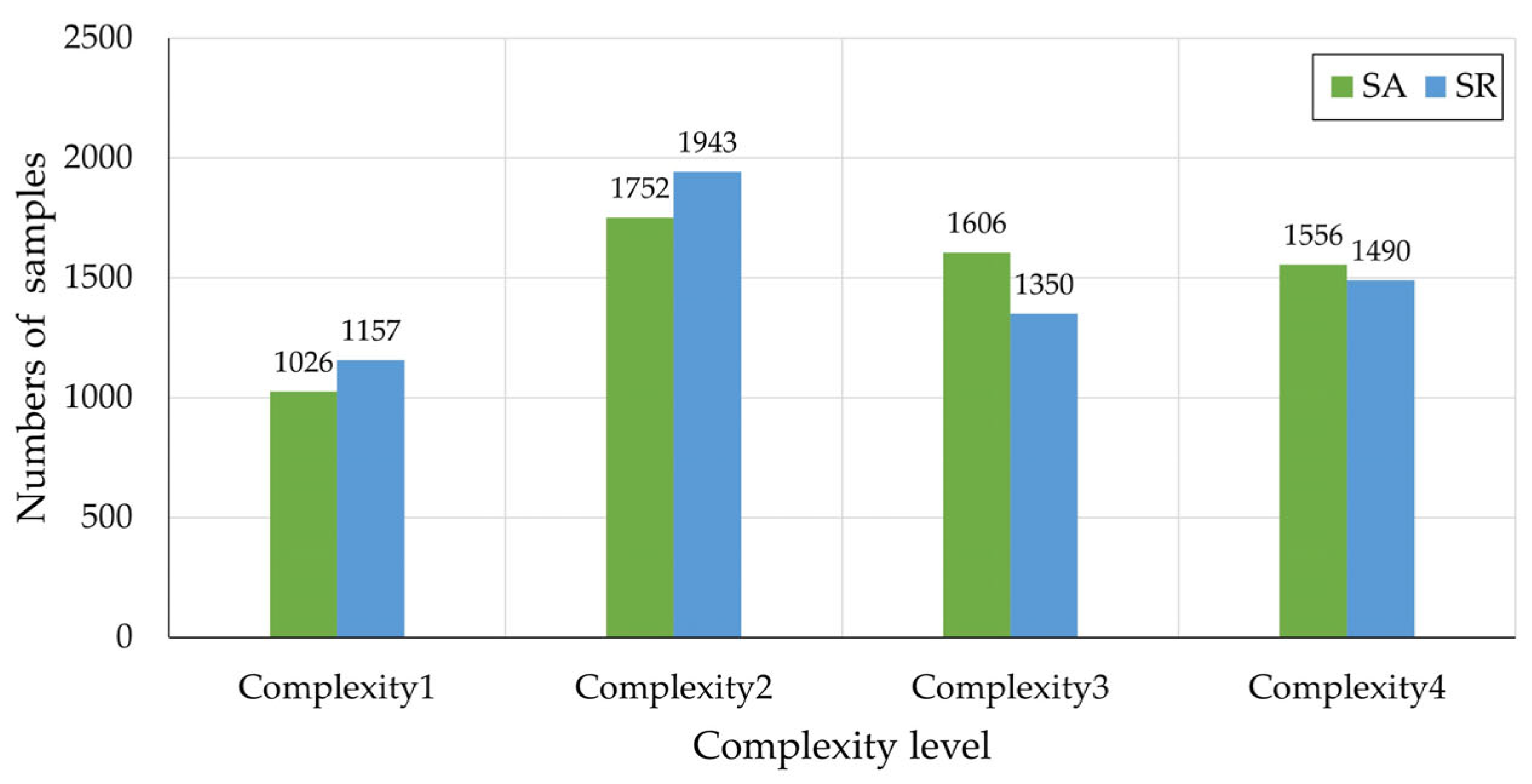
• In conclusion, on the three performance criteria ($MAE$, $ACC$, and $Macro\text{-}F1\text{-}score$), the GNN-based approaches perform better than the hand-crafted feature methods, with our HGRL achieving the best results. The primary distinction between the two types of approaches resides in their respective used features. Among these, the GNN-based technique automatically extracts characteristics from ATSGs using neural networks with various architectures. Figure 9 provides a good illustration of the experimental sample data distribution. In SA and SR, the proportion of CL-level samples is roughly 5:9:8:8 and 4:6:4:5, respectively. The Macro-F1-score was chosen as the performance indicator since there are a substantial number of samples in each category—nearly 6000—despite the fact that the value distribution is not perfectly balanced. Owing to the rather uniform distribution of the dataset, the $Macro\text{-}F1\text{-}score$ and $Acc$ do not differ much (the production of the $F1\text{-}score$ takes into account the data distribution in situations involving severely unbalanced datasets).
• Possible reasons for the BPNN and SVM’s poor performance involve: the chosen indicators are not appropriate to the sectors in the experiment and cannot correctly capture the dynamic flight information in the sectors. The static structure and traffic operation of various airspaces may be highly varied, which may result in varying operational complexity feature sets applicable to various sectors. Consequently, it is obviously inappropriate to develop a collection of immutable complexity feature index systems for application in different airspace sectors. The outcome reveals that the current hand-crafted features may be inadequate for depicting sector complexity, and that the GNN-based technique may extract useful information from the produced ATSGs.
• The built ATSG can properly represent the variables that influence the sector’s complexity. As can be seen, the $ACC$ of the global pooling group was almost 10% more than that of the prior group. The GCN has the best performance in both the SA and SR sectors in the global pooling group, with $ACC$ exceeding 76%. However, we also find that the global pooling group is unable to provide satisfactory outcomes. We believe that the primary cause is that when merging node representations universally, the ATSG structure feature is ignored, which is the most important factor in revealing aircraft awareness of the conflict. This further validates the need for adding the hierarchical pooling module.
• Hierarchical feature extraction helps significantly minimize information loss during the ATSG’s feature extraction procedure. In the third category, the listed approaches prevent sub-graph structure loss or even misrepresentation produced by the single-time pooling method, which compresses all node characteristics into a single graph feature vector. Obviously, they improve classification performance significantly. We see that hierarchical pooling models may attain relative superior performance compared to the majority of baselines, demonstrating the efficacy of the hierarchical pooling strategy. ASAP outperforms its competition, a sparse and differentiable pooling approach that utilizes an improved GNN formulation to determine the significance of every single node in a certain graph. Clearly, our suggested HGRL performs better than ASAP across all evaluation measures.
• The incorporation of ATCOI may effectively enhance the performance of the suggested classification model; the $ACC$ of HGRL in SA even surpassed 90%. Comparing the experimental results of HGRL-NCI and HGRL reveals that the combination of airspace traffic situation information and ATCOI has a greater effect than using only trajectory data. Due to the fact that the combination of the two includes more information and may have a synergistic impact to jointly portray the sector’s complexity, the combination of them is preferable. Furthermore, ATCOI is directly tied to the ATC workload, resulting in a more precise categorization of sector CL.
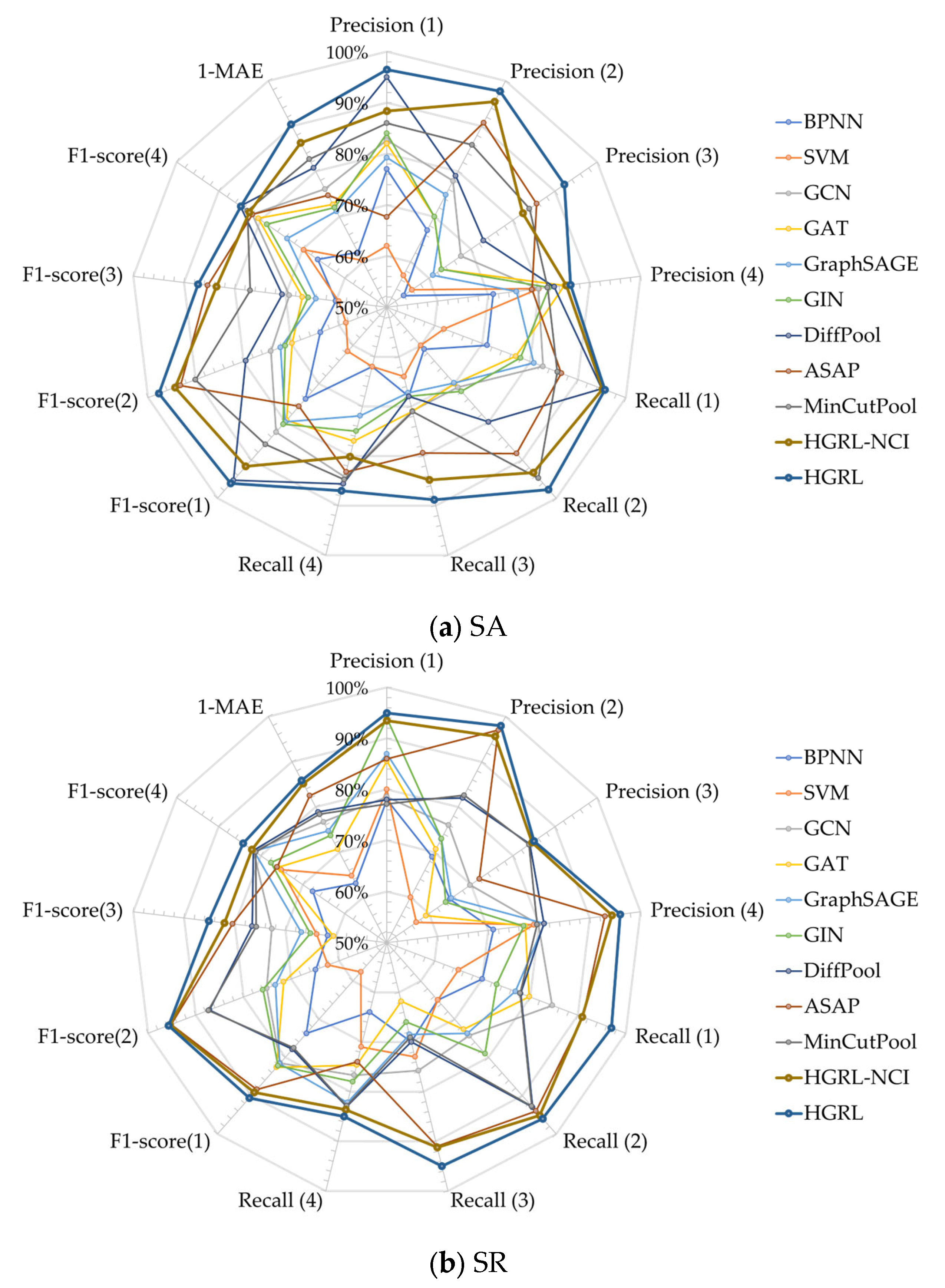
• HGRL can mitigate the issue of class imbalance to some degree. The radar map (Figure 11) reveals that the two biggest polygon areas are based on HGRL structure. In contrast, the outcomes of other approaches suffer from sample set class-imbalance. Compared to CL1 and CL2, CL3 and CL4 generate a greater workload and are among the few severe instances seen in normal work. Consequently, numerous baselines’ performance on CL3 and CL4 has been unstable. Our suggested model outperforms the competition in terms of both overall performance and each CL degree. At the same time, HGRL can still obtain a relatively higher precision despite the imbalance of samples in sectors with various functions, demonstrating that our methodology has significant generalization potential. Even without the additional characterization provided by ATCOI, the HGRL received an excellent evaluation performance. The identification accuracy was as high as 88.05%, beating by a wide margin machine learning algorithms that employ conventional criteria.

5. Conclusions

This research provides a graph-based approach to air traffic complexity assessment capable of automatically extracting abstract traffic aspects for ATS topology learning. First, the ATS is converted into an ATSG, properly representing all of the information that is available at the location in space and the approach pattern between aircraft. The second step is to use a HGRL architecture to gather information about airspace operating difficulty based on the generated ATSG and conduct an airspace complexity assessment.

The ATSG is able to accurately depict the factors that contribute to the complexity of the sector. During the process of ATSG’s feature extraction, hierarchical feature extraction is able to considerably reduce the amount of information that is lost. The ways that are presented avoid the loss of the sub-graph structure or even the misrepresentation that is created by the single-time pooling method. This method compiles all of the node characteristics into a single graph feature vector. It should come as no surprise that they greatly increase categorization performance. The fact that hierarchical pooling models may achieve somewhat greater performance compared to the majority of baselines demonstrates the efficacy of the hierarchical pooling technique. We can observe this by comparing the results of hierarchical pooling models to the results of baselines. In the meantime, the addition of ATCOI might improve the performance of the suggested classification model. All other well-known machine learning approaches were surpassed by our approach, and the ATCOI integration showed positive outcomes in experimental evaluations. The generalizability of our proposed model has been thoroughly tested, and it outperforms conventional feature factor set-based approaches in both the SA and SR sectors.

The experimental data demonstrate that HGRL significantly outperforms machine learning approaches employing conventional metrics, regardless of whether the airspace is evaluated based solely on the aircraft’s flight data (HGRL-NCI) or by fusing ATCOI, and that the newly proposed network structure outperforms previous structures. We can conclude that our FCN can accurately identify both actual and potential conflicts. Despite a slight variance caught between the simulated ATCOI employed and true instructions in terms of their amount and type, the fusion of both objective and subjective factors for assessing sector complexity has been demonstrated to be more effective than solely focusing on a singular aspect. Notwithstanding the primary factor influencing the sector complexity is the aircraft’s trajectory (objective factor), the controller’s subjective intervention could also impact the airspace situation. Our paper provides an initial exploration and validation of this idea.

Our high-precision, real-time technique for assessing complexity can expedite and improve controllers’ decision making. The trained model can be used directly for real-time airspace situational assessment, which is an accurate tool for resolving problems that can arise when controllers incorrectly assess the overall airspace situation, miss key aircraft groups, forget the historical sector CL, or experience other control issues. HGRL is an effective control decision aid that may be utilized for both real-time evaluation and post-event analysis. In order to prevent events such as the “Überlingen mid-air collision,” the ATM industry need more precise ATC decision support tools, and our proposed approach has been proven to be beneficial.

In future work, we will incorporate data from different FIRs to validate the model’s generalizability in depth. Although SA and SR in the Wuhan FIR are rather typical and may demonstrate the superiority of HGRL to some extent, the diversity of sector forms and states needs more case studies. In addition, the incorporation of real ATCOI data will enhance the attribute characterization of ATSGs, and the combination of automatic ATCOI speech recognition (there have already been various researches on ATCOI speech recognition [54,55,56,57,58]) and a complexity assessment model will become an integral part of intelligent ATM under ideal conditions, which is also one of our future research directions. With the increasing growth of the aviation industry, the CL may need to be subdivided more precisely, and the 1-min interval for determining ATS may need to be enhanced. Weather conditions and flight schedules in the sector can be used as multi-source information to capture time-dependent characteristics for sector complexity classification from a macroscopic perspective. In addition, as a result of the shift in the structure of the sector’s features, we will apply more powerful neural network modules, such as the transformer and attention mechanism, for enhancement.

References

1. Rescher, N. Complexity: A Philosophical Overview; Transaction Publishers: New Jersey, NJ, USA, 1998; ISBN 978-1-4128-2008-0. [Google Scholar]
2. Stacey, R.D. The Science of Complexity: An Alternative Perspective for Strategic Change Processes. Strateg. Manag. J. 1995, 16, 477–495. [Google Scholar] [CrossRef]
3. Lissack, M.R. Complexity: The Science, Its Vocabulary, and Its Relation to Organizations. Emergence 1999, 1, 110–126. [Google Scholar] [CrossRef]
4. Mogford, R.; Guttman, J.; Morrow, S.; Kopardekar, P. The Complexity Construct in Air Traffic Control A Review and Synthesis of the Literature; (DOTFAA-CT TN9522); Atl. City NJ FAA; Federal Aviation Administration: Washington, DC, USA, 1995.
5. Meckiff, C.; Chone, R.; Nicolaon, J.-P. The Tactical Load Smoother for Multi-Sector Planning. In Proceedings of the 2nd USA/Europe Air Traffic Management R&D Seminar, Orlando, FL, USA, 1–4 December 1998. [Google Scholar]
6. Chatterji, G.; Sridhar, B. Measures for Air Traffic Controller Workload Prediction. In Proceedings of the 1st AIAA, Aircraft, Technology Integration, and Operations Forum, Los Angeles, CA, USA, 16 October 2001; American Institute of Aeronautics and Astronautics. [Google Scholar]
7. Radišić, T.; Novak, D.; Juričić, B. Reduction of Air Traffic Complexity Using Trajectory-Based Operations and Validation of Novel Complexity Indicators. IEEE Trans. Intell. Transp. Syst. 2017, 18, 3038–3048. [Google Scholar] [CrossRef]
8. Bloem, M.; Gupta, P. Configuring Airspace Sectors with Approximate Dynamic Programming. In Proceedings of the International Congress of the Aeronautical Sciences, Nice, France, 19–24 September 2010. [Google Scholar]
9. Moon, W.-C.; Yoo, K.-E.; Choi, Y.-C. Air Traffic Volume and Air Traffic Control Human Errors. J. Transp. Technol. 2011, 1, 47. [Google Scholar] [CrossRef]
10. Abdul Rahman, S.M.; Mulder, M.; van Paassen, R. Using the Solution Space Diagram in Measuring the Effect of Sector Complexity during Merging Scenarios. In Proceedings of the AIAA Guidance, Navigation, and Control Conference, Portland, OR, USA, 8–11 August 2011; p. 6693. [Google Scholar]
11. Song, Z.; Chen, Y.; Li, Z.; Zhang, D.; Bi, H. A Review for Workload Measurement of Air Traffic Controller Based on Air Traffic Complexity. In Proceedings of the 25th Chinese Control and Decision Conference (CCDC), Guiyang, China, 25–27 May 2013; IEEE: Piscataway Township, NJ, USA; pp. 2107–2112. [Google Scholar]
12. Loft, S.; Pearcy, B.; Remington, R.W. Varying the Complexity of the Prospective Memory Decision Process in an Air Traffic Control Simulation. Z. Psychol. 2015, 219, 77–84. [Google Scholar] [CrossRef]
13. Alexandrov, N. Control of Future Air Traffic Systems via Complexity Bound Management. In Proceedings of the 2013 Aviation Technology, Integration, and Operations Conference, Los Angeles, CA, USA, 12–14 August 2013; p. 4419. [Google Scholar]
14. Corver, S.C.; Unger, D.; Grote, G. Predicting Air Traffic Controller Workload: Trajectory Uncertainty as the Moderator of the Indirect Effect of Traffic Density on Controller Workload through Traffic Conflict. Hum. Factors 2016, 58, 560–573. [Google Scholar] [CrossRef]
15. Tang, J.; Alam, S.; Lokan, C.; Abbass, H.A. A Multi-Objective Approach for Dynamic Airspace Sectorization Using Agent Based and Geometric Models. Transp. Res. Part C Emerg. Technol. 2012, 21, 89–121. [Google Scholar] [CrossRef]
16. Kontogiannis, T.; Malakis, S. Strategies in Coping with Complexity: Development of a Behavioural Marker System for Air Traffic Controllers. Saf. Sci. 2013, 57, 27–34. [Google Scholar] [CrossRef]
17. Hong, Y.; Kim, Y.; Lee, K. Application of Complexity Assessment for Conflict Resolution in Air Tra [|# 14#|] Ffic Management Systems. In Proceedings of the AIAA Guidance, Navigation, and Control (GNC) Conference, Boston, MA, USA, 19–22 August 2013; p. 4625. [Google Scholar]
18. Schmidt, D.K. On Modeling ATC Work Load and Sector Capacity. J. Aircr. 1976, 13, 531–537. [Google Scholar] [CrossRef]
19. Next Generation Air Transportation System (NextGen)|Federal Aviation Administration. Available online: https://www.faa.gov/nextgen (accessed on 14 March 2023).
20. Single European Sky. Available online: https://transport.ec.europa.eu/transport-modes/air/single-european-sky_en (accessed on 14 March 2023).
21. Edwards, T.; Homola, J.; Mercer, J.; Claudatos, L. Multifactor Interactions and the Air Traffic Controller: The Interaction of Situation Awareness and Workload in Association with Automation. Cogn. Technol. Work 2017, 19, 687–698. [Google Scholar] [CrossRef] [Green Version]
22. Triyanti, V.; Azis, H.A.; Iridiastadi, H.; Yassierli. Workload and Fatigue Assessment on Air Traffic Controller. IOP Conf. Ser. Mater. Sci. Eng. 2020, 847, 012087. [Google Scholar] [CrossRef]
23. Delahaye, D.; Paimblanc, P.; Puechmorel, S.; Histon, J.M.; Hansman, R.J. A New Air Traffic Complexity Metric Based on Dynamical System Modelization. In Proceedings of the 21st Digital Avionics Systems Conference, Irvine, CA, USA, 27–31 October 2002; Volume 1, p. 4A2. [Google Scholar]
24. Delahaye, D.; Puechmorel, S.; Hansman, J.; Histon, J. Air Traffic Complexity Map Based on Non Linear Dynamical Systems. Air Traffic Control Q. 2004, 12, 367–388. [Google Scholar] [CrossRef]
25. Puechmorel, S.; Delahaye, D. New Trends in Air Traffic Complexity. In Proceedings of the EIWAC 2009, ENRI International Workshop on ATM/CNS, Tokyo, Japan, 5–6 March 2009; p. 55. [Google Scholar]
26. Delahaye, D.; Puechmorel, S. 4D Trajectories Complexity Metric Based on Lyapunov Exponents. In Proceedings of the ECCS 2011, European Conference on Complex Systems, Vienne, Austria, 12 September 2011. [Google Scholar]
27. Lee, K.; Feron, E.; Pritchett, A. Air Traffic Complexity: An Input-Output Approach. In Proceedings of the 2007 American Control Conference, New York, NY, USA, 9–13 July 2007; pp. 474–479. [Google Scholar]
28. Lee, K.; Feron, E.; Pritchett, A. Describing Airspace Complexity: Airspace Response to Disturbances. J. Guid. Control Dyn. 2009, 32, 210–222. [Google Scholar] [CrossRef]
29. Hong, Y.; Kim, Y.; Lee, K. Conflict Management in Air Traffic Control Using Complexity Map. J. Aircr. 2015, 52, 1524–1534. [Google Scholar] [CrossRef]
30. Prandini, M.; Putta, V.; Hu, J. A Probabilistic Measure of Air Traffic Complexity in 3-D Airspace. Int. J. Adapt. Control Signal Process. 2010, 24, 813–829. [Google Scholar] [CrossRef]
31. Prandini, M.; Putta, V.; Hu, J. Air Traffic Complexity in Future Air Traffic Management Systems. J. Aerosp. Oper. 2012, 1, 281–299. [Google Scholar] [CrossRef]
32. Laudeman, I.V.; Shelden, S.G.; Branstrom, R.; Brasil, C. Dynamic Density: An Air Traffic Management Metric; NASA: Washington, DC, USA, 1998.
33. Gianazza, D. Forecasting Workload and Airspace Configuration with Neural Networks and Tree Search Methods. Artif. Intell. 2010, 174, 530–549. [Google Scholar] [CrossRef] [Green Version]
34. Xiao, M.; Zhang, J.; Cai, K.; Cao, X. ATCEM: A Synthetic Model for Evaluating Air Traffic Complexity: ATCEM: A Synthetic Model for Evaluating Air Traffic Complexity. J. Adv. Transp. 2016, 50, 315–325. [Google Scholar] [CrossRef] [Green Version]
35. Zhu, X.; Cai, K.; Cao, X. A Semi-Supervised Learning Method for Air Traffic Complexity Evaluation. In Proceedings of the 2017 Integrated Communications, Navigation and Surveillance Conference (ICNS), Herndon, VI, USA, 18–20 April 2017; pp. 1A3-1–1A3-11. [Google Scholar]
36. Cao, X.; Zhu, X.; Tian, Z.; Chen, J.; Wu, D.; Du, W. A Knowledge-Transfer-Based Learning Framework for Airspace Operation Complexity Evaluation. Transp. Res. Part C Emerg. Technol. 2018, 95, 61–81. [Google Scholar] [CrossRef]
37. Li, B.; Du, W.; Zhang, Y.; Chen, J.; Tang, K.; Cao, X. A Deep Unsupervised Learning Approach for Airspace Complexity Evaluation. IEEE Trans. Intell. Transp. Syst. 2021, 23, 11739–11751. [Google Scholar] [CrossRef]
38. Xie, H.; Zhang, M.; Ge, J.; Dong, X.; Chen, H. Learning Air Traffic as Images: A Deep Convolutional Neural Network for Airspace Operation Complexity Evaluation. Complexity 2021, 2021, 6457246. [Google Scholar] [CrossRef]
39. Tan, X.; Sun, Y.; Zeng, W.; Quan, Z. Congestion Recognition of the Air Traffic Control Sector Based on Deep Active Learning. Aerospace 2022, 9, 302. [Google Scholar] [CrossRef]
40. Song, L.; Wanke, C.; Greenbaum, D. Predicting Sector Capacity for Tfm Decision Support. In Proceedings of the 6th AIAA Aviation Technology, Integration and Operations Conference (ATIO), Wichita, KS, USA, 25–27 September 2006; p. 7827. [Google Scholar]
41. Gianazza, D. Airspace Configuration Using Air Traffic Complexity Metrics. In Proceedings of the ATM 2007, 7th USA/Europe Air Traffic Management Research and Developpment Seminar, Barcelona, Spain, 2 July 2007. [Google Scholar]
42. Gianazza, D.; Guittet, K. Selection and Evaluation of Air Traffic Complexity Metrics. In Proceedings of the 2006 IEEE/AIAA 25TH Digital Avionics Systems Conference, Portland, OR, USA, 15–19 October 2006; pp. 1–12. [Google Scholar]
43. Cook, A.; Blom, H.A.; Lillo, F.; Mantegna, R.N.; Micciche, S.; Rivas, D.; Vázquez, R.; Zanin, M. Applying Complexity Science to Air Traffic Management. J. Air Transp. Manag. 2015, 42, 149–158. [Google Scholar] [CrossRef] [Green Version]
44. Wang, H.; Song, Z.; Wen, R.; Zhao, Y. Study on Evolution Characteristics of Air Traffic Situation Complexity Based on Complex Network Theory. Aerosp. Sci. Technol. 2016, 58, 518–528. [Google Scholar] [CrossRef]
45. Yang, L.; Yin, S.; Hu, M.; Han, K.; Zhang, H. Empirical Exploration of Air Traffic and Human Dynamics in Terminal Airspaces. Transp. Res. Part C Emerg. Technol. 2017, 84, 219–244. [Google Scholar] [CrossRef] [Green Version]
46. Zhu, X.; Cao, X.; Cai, K. Measuring Air Traffic Complexity Based on Small Samples. Chin. J. Aeronaut. 2017, 30, 1493–1505. [Google Scholar] [CrossRef]
47. Kipf, T.N.; Welling, M. Semi-Supervised Classification with Graph Convolutional Networks. arXiv 2016, arXiv:1609.02907. [Google Scholar]
48. Tang, J.; Wang, Y.; Liu, F. Characterizing Traffic Time Series Based on Complex Network Theory. Phys. A Stat. Mech. Appl. 2013, 392, 4192–4201. [Google Scholar] [CrossRef]
49. Tang, J.; Wang, Y.; Wang, H.; Zhang, S.; Liu, F. Dynamic Analysis of Traffic Time Series at Different Temporal Scales: A Complex Networks Approach. Phys. A Stat. Mech. Appl. 2014, 405, 303–315. [Google Scholar] [CrossRef]
50. Wen, X.; Tu, C.; Wu, M. Node Importance Evaluation in Aviation Network Based on “No Return” Node Deletion Method. Phys. A Stat. Mech. Appl. 2018, 503, 546–559. [Google Scholar] [CrossRef]
51. Wen, X.; Tu, C.; Wu, M.; Jiang, X. Fast Ranking Nodes Importance in Complex Networks Based on LS-SVM Method. Phys. A Stat. Mech. Appl. 2018, 506, 11–23. [Google Scholar] [CrossRef]
52. Jiang, X.; Wen, X.; Wu, M.; Song, M.; Tu, C. A Complex Network Analysis Approach for Identifying Air Traffic Congestion Based on Independent Component Analysis. Phys. A Stat. Mech. Appl. 2019, 523, 364–381. [Google Scholar] [CrossRef]
53. Gianazza, D.; Guittet, K. Évaluation of Air Traffic Complexity Metrics Using Neural Networks and Sector Status. In Proceedings of the 2nd International Conference on Research in Air Transportation, Belgrade, Serbia, 24 June 2006. [Google Scholar]
54. Lin, Y. Spoken Instruction Understanding in Air Traffic Control: Challenge, Technique, and Application. Aerospace 2021, 8, 65. [Google Scholar] [CrossRef]
55. Lin, Y.; Yang, B.; Li, L.; Guo, D.; Zhang, J.; Chen, H.; Zhang, Y. ATCSpeechNet: A Multilingual End-to-End Speech Recognition Framework for Air Traffic Control Systems. Appl. Soft Comput. 2021, 112, 107847. [Google Scholar] [CrossRef]
56. Fan, P.; Guo, D.; Lin, Y.; Yang, B.; Zhang, J. Speech Recognition for Air Traffic Control via Feature Learning and End-to-End Training. arXiv 2021, arXiv:2111.02654. [Google Scholar] [CrossRef]
57. Zhang, J.; Zhang, P.; Guo, D.; Zhou, Y.; Wu, Y.; Yang, B.; Lin, Y. Automatic Repetition Instruction Generation for Air Traffic Control Training Using Multi-Task Learning with an Improved Copy Network. Knowl. Based Syst. 2022, 241, 108232. [Google Scholar] [CrossRef]
58. Lin, Y.; Ruan, M.; Cai, K.; Li, D.; Zeng, Z.; Li, F.; Yang, B. Identifying and Managing Risks of AI-Driven Operations: A Case Study of Automatic Speech Recognition for Improving Air Traffic Safety. Chin. J. Aeronaut. 2022, in press. [Google Scholar] [CrossRef]
59. Isufaj, R.; Koca, T.; Piera, M.A. Spatiotemporal Graph Indicators for Air Traffic Complexity Analysis. Aerospace 2021, 8, 364. [Google Scholar] [CrossRef]
60. Martins, A.F.T.; Astudillo, R.F. From Softmax to Sparsemax: A Sparse Model of Attention and Multi-Label Classification. arXiv 2016, arXiv:1602.02068. [Google Scholar]
61. Yan, Z.; Yang, H.; Li, F.; Lin, Y. A Deep Learning Approach for Short-Term Airport Traffic Flow Prediction. Aerospace 2022, 9, 11. [Google Scholar] [CrossRef]
62. Grandini, M.; Bagli, E.; Visani, G. Metrics for Multi-Class Classification: An Overview. arXiv 2020, arXiv:2008.05756. [Google Scholar]
63. An, J.; Guo, L.; Liu, W.; Fu, Z.; Ren, P.; Liu, X.; Li, T. IGAGCN: Information Geometry and Attention-Based Spatiotemporal Graph Convolutional Networks for Traffic Flow Prediction. Neural Netw. 2021, 143, 355–367. [Google Scholar] [CrossRef] [PubMed]
64. Hamilton, W.; Ying, R.; Leskovec, J. Inductive Representation Learning on Large Graphs. arXiv 2017, arXiv:1706.02216. [Google Scholar]
65. Xu, K.; Hu, W.; Leskovec, J.; Jegelka, S. How Powerful Are Graph Neural Networks? arXiv 2019, arXiv:1810.00826. [Google Scholar]
66. Ying, R.; You, J.; Morris, C.; Ren, X.; Hamilton, W.L.; Leskovec, J. Hierarchical Graph Representation Learning with Differentiable Pooling. In Proceedings of the 32nd International Conference on Neural Information Processing Systems, Montreal, QC, Canada, 3 December 2018; Curran Associates Inc.: Red Hook, NY, USA; pp. 4805–4815. [Google Scholar]
67. Ranjan, E.; Sanyal, S.; Talukdar, P. ASAP: Adaptive Structure Aware Pooling for Learning Hierarchical Graph Representations. Proc. AAAI Conf. Artif. Intell. 2020, 34, 5470–5477. [Google Scholar] [CrossRef]
68. Bianchi, F.M.; Grattarola, D.; Alippi, C. Spectral Clustering with Graph Neural Networks for Graph Pooling. In Proceedings of the 37th International Conference on Machine Learning, Virtual Event, 13 July 2020; pp. 874–883. [Google Scholar]
Figure 1. HGRL architecture for sector complexity evaluation.
Aerospace 10 00352 g001
Figure 2. A simplified radar screen of ZHHH SA, Wuhan FIR.
Aerospace 10 00352 g002
Figure 3. Abstract example of ATCOI combined with ATS.
Aerospace 10 00352 g003
Figure 4. Coarse granulation classification of ATCOI in the proposed model.
Aerospace 10 00352 g004
Figure 5. Ellipsoidal flight protection zone.
Aerospace 10 00352 g005
Figure 6. Proximity calculation.
Aerospace 10 00352 g006
Figure 7. Details of structure learning mechanism.
Aerospace 10 00352 g007
Figure 8. Part of Wuhan FIR regulated by Civil Aviation Administration of China (CAAC).
Aerospace 10 00352 g008
Figure 9. Basic information of 2 experimental sectors.
Aerospace 10 00352 g009
Figure 10. Network parameter sensitivity analysis.
Aerospace 10 00352 g010
Figure 11. Evaluation performance of different methods of SA and SR in radar chart.
Aerospace 10 00352 g011