Article

Adaptive Mode Filter for Lamb Wavefield in the Wavenumber-Time Domain Based on Wavenumber Response Function

by
Muhamad Azim Azhad Shahrim
1,
Chen Ciang Chia
2,
Hafiz Rashidi Ramli
3,
Mohammad Yazdi Harmin
1,* and
Jung-Ryul Lee
2,*
1
Department of Aerospace Engineering, Universiti Putra Malaysia, Serdang 43400, Selangor, Malaysia
2
Department of Aerospace Engineering, KAIST, Daejeon 34141, Republic of Korea
3
Department of Electrical and Electronic Engineering, Universiti Putra Malaysia, Serdang 43400, Selangor, Malaysia
*
Authors to whom correspondence should be addressed.
Aerospace 2023, 10(4), 347; https://doi.org/10.3390/aerospace10040347
Submission received: 3 February 2023 / Revised: 18 March 2023 / Accepted: 25 March 2023 / Published: 3 April 2023

Abstract

:
Aerospace thin-walled structures are susceptible to various forms of damage and they can be effectively inspected using Lamb wavefields. However, Lamb wavefields contain at least two dispersive modes which interfere with the generation of a clear image for damage visualization. Conventional mode filters produce inconsistent results due to the need for the ad hoc or manual adjustment of the processing parameters by experienced users. An automatic, adaptive mode filter is proposed to remove human subjectivity, thereby improving the consistency of the results and making it more practical to utilize. It converts the wavefield from the space-time domain to the wavenumber-time domain and then consolidates the data in the time and angular axes into a wavenumber response function (WRF) where the modes can be automatically isolated. The single-mode data were converted back into space-time domain for result visualization. Its effectiveness was experimentally proven by keeping 78.2–122.0% of energy for a wanted mode and suppressing the energy of an unwanted mode to 0.1–4.5%. Its automatic adaptability was demonstrated through the improved visibility of a blind hole, corrosion, water-ingress in honeycomb panel, and impact damage in a complex composite wing. Consistent results can be generated in a highly efficient manner while significantly reducing the computational workload and hardware requirements.

1. Introduction

Aerospace structures have been optimized to increase the strength-to-weight ratio through thin-wall design principles, innovative design concepts, and alternative materials [1,2,3,4,5,6,7,8,9]. However, maintenance for safety and reliability becomes critical due to their complex structural design [5,10]. To prevent catastrophic failure, aerospace structures require periodic in-depth inspections using non-destructive testing (NDT) technology to detect hidden damage such as corrosion, cracks, delamination, and debonding [11,12,13,14,15]. In this regard, ultrasonic inspection has been historically relied on for its capability to inspect through the thickness of structural walls for damage detection [16,17,18]. Among various ultrasonic techniques, guided ultrasonic wave propagation imaging (G-UPI) [19] has emerged as a significant technique in recent years.
The G-UPI system inspects thin-walled structures by generating and sensing Lamb waves [20,21] at densely distributed grid points over the target surface. These waves can be altered by local damage and the changes can be extracted using a suitable result processing algorithm for damage visualization and evaluation [22,23]. However, Lamb waves contain infinite modes that are dispersive and overlapping in space and time [24,25], which can complicate feature extraction [26,27]. Although generating and sensing a specific mode has been investigated [28,29,30,31,32], the requirement for specialized transducers or conditions has limited its wider use. To date, only the mode cut-off method based on frequency bandpass has been universally adopted to limit the modes to the fundamental S0 and A0 modes.
The separation of the remaining modes requires further signal processing. Alleyne and Cawley [33] found that two-dimensional (2D) Fourier transform (FT) could be used to resolve the individual mode of Lamb waves. Ruzzene [34] extended it for the directional filtering of Lamb waves in the three-dimensional (3D) wavenumber-frequency domain. Kudela et al. [35] proposed the removal of all incident modes and keeping only the damage-related “anomalous waves/mode” [36,37,38]. This method is faster and more robust as it only involves 2D FT and can effectively remove incident modes regardless of the propagation direction of the waves. It is, however, critical to generate a suitable incident filter that is averaged from the first few time-indexed frames of the wavenumber-time data before the incident waves encounter any damage. Meeting this requirement is tricky as the wavefield source must be positioned at an optimal distance from potential damage. If the source is too close, the number of frames for averaging becomes insufficient, and if it is too far and positioned outside the region of interest, the faster-travel mode may encounter damage before the other, leading to ineffective removal of all incident modes. Using these directional or incident filters for complex thin-walled structures is not practical because waves phenomena, including reflections, scatterings, and mode conversions, caused by both benign structural components and damage are indistinguishable. Modes removal can also be performed in the wavenumber-frequency domain [39], but this is generally slower due to 3D FT.
For complex thin-walled structures, isolating a specific wave mode for structural imaging is a more promising strategy. The filtered single-mode data can be processed for detailed analysis, such as for the visualization of specimen thickness instead of any arbitrary intensity or amplitude. Mode filtering in the wavenumber-frequency domain has also been proposed and used [40,41,42,43,44,45]. The filter generally involves the bandpass of the data in the frequency and wavenumber domains using respective filter windows. The suitability of the windows depends at least on two aspects. Firstly, the central position of the windows must be adjusted according to the energy peak of the mode of interest. Secondly, the width of the filter windows must be large to isolate most of the energy of a selected mode but not too large so that the energy of other modes is included [40]. Apparently, these two aspects are complicated by the dispersive nature of the waves, i.e., the position and width of the wavenumber filter windows are frequency-, material-, and damage-type-dependent. Moreover, setting the window width is a subjective task due to the lack of a clear boundary between modes. This implies that good skills and knowledge are needed for the ad hoc optimization of the mode-filtering process and to cater to different specimens and datasets. A direct consequence of any ad hoc processing, especially when performed by different users, is the inconsistency of the results. Another consequence is the need to perform multiple runs of the algorithm in pursuit of the best result, which is computationally burdensome due to multiple forward and inverse 3D FT computations.
The motivation for this work was to keep the advantages of the above-mentioned filters and at the same time circumvent their disadvantages. We proposed an adaptive mode filter in the wavenumber-time domain based on our preliminary work reported in [46] to harness the following advantages. Firstly, it can be used to isolate a specific incident mode of interest, thus facilitating further mode analysis for the structural imaging of complex structures. It also provides the flexibility to remove all incident modes, thus only keeping the anomalous mode for easy damage visualization. Secondly, the proposed method has high adaptability to the data frequency, specimen material, and damage type. Note that this is the most significant contribution of the proposed method. With this adaptability, mode isolation or removal can be performed automatically without any ad hoc tinkering towards the algorithm or manual adjustment of the processing parameters such as the width of the filter window. Thirdly, the proposed method guarantees consistent results as a direct consequence of needing no ad hoc adjustment, regardless of who processes the data or how many times these are processed. Fourthly, the proposed method is fast due to the adoption of 2D FT instead of 3D FT. This greatly reduces the computation burden and hardware requirements.
This article is organized as follows. Section 2 describes the proposed adaptive mode filter. The characteristics and advantages of the proposed method are then experimentally demonstrated using the materials and setup described in Section 3. Specimens made of different materials and containing different types of damage were used to demonstrate the adaptability of the proposed method. The results and discussions are presented in Section 4, and lastly the concluding remarks and further works are given in Section 5.

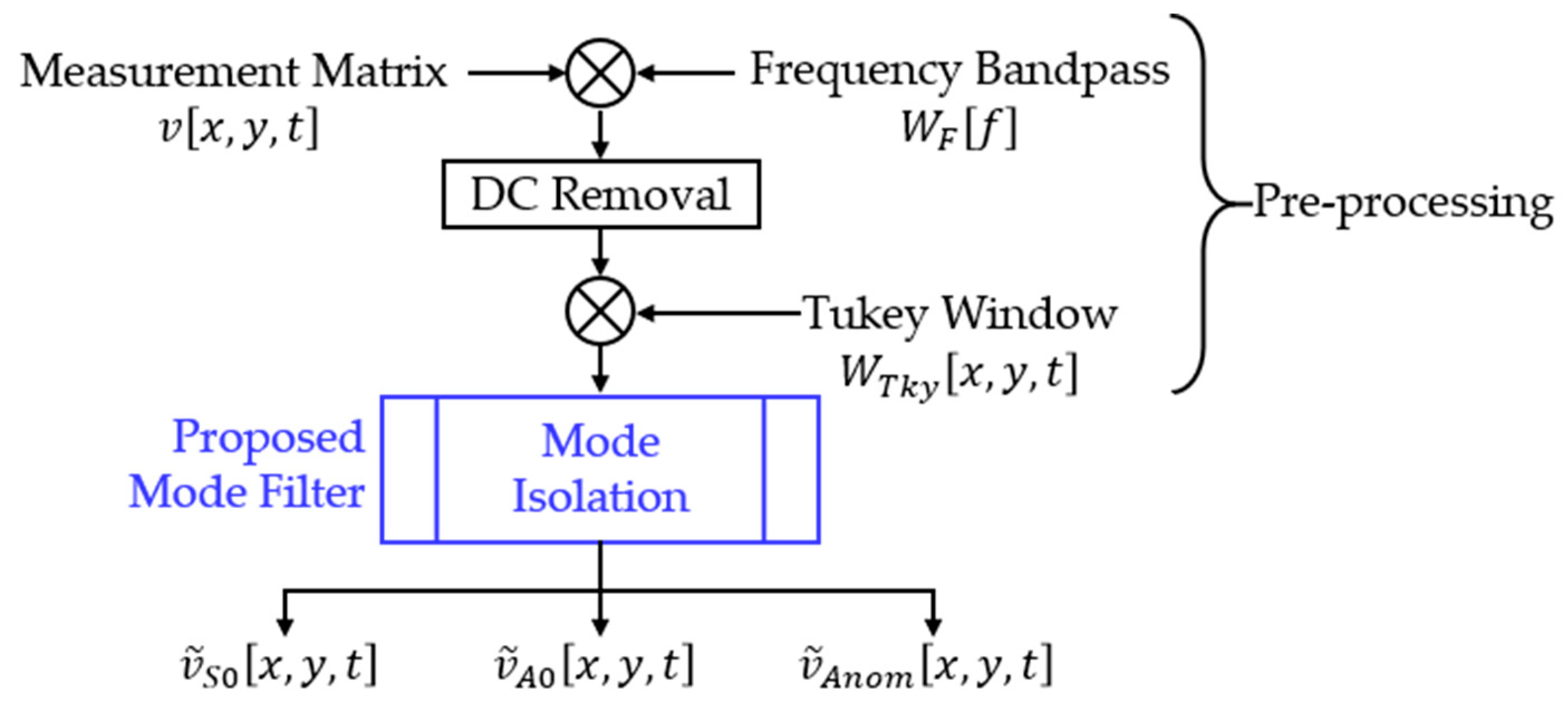
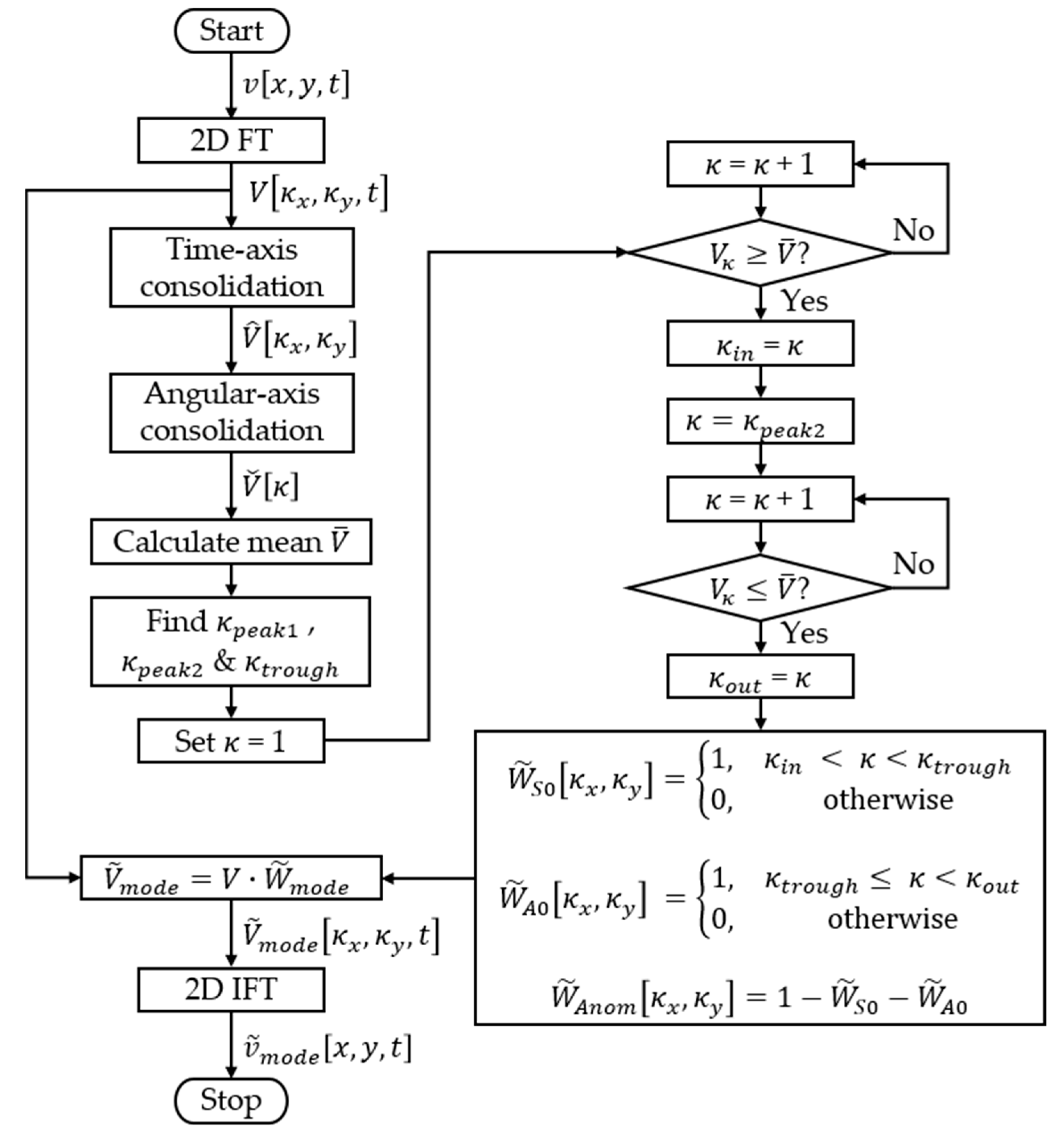
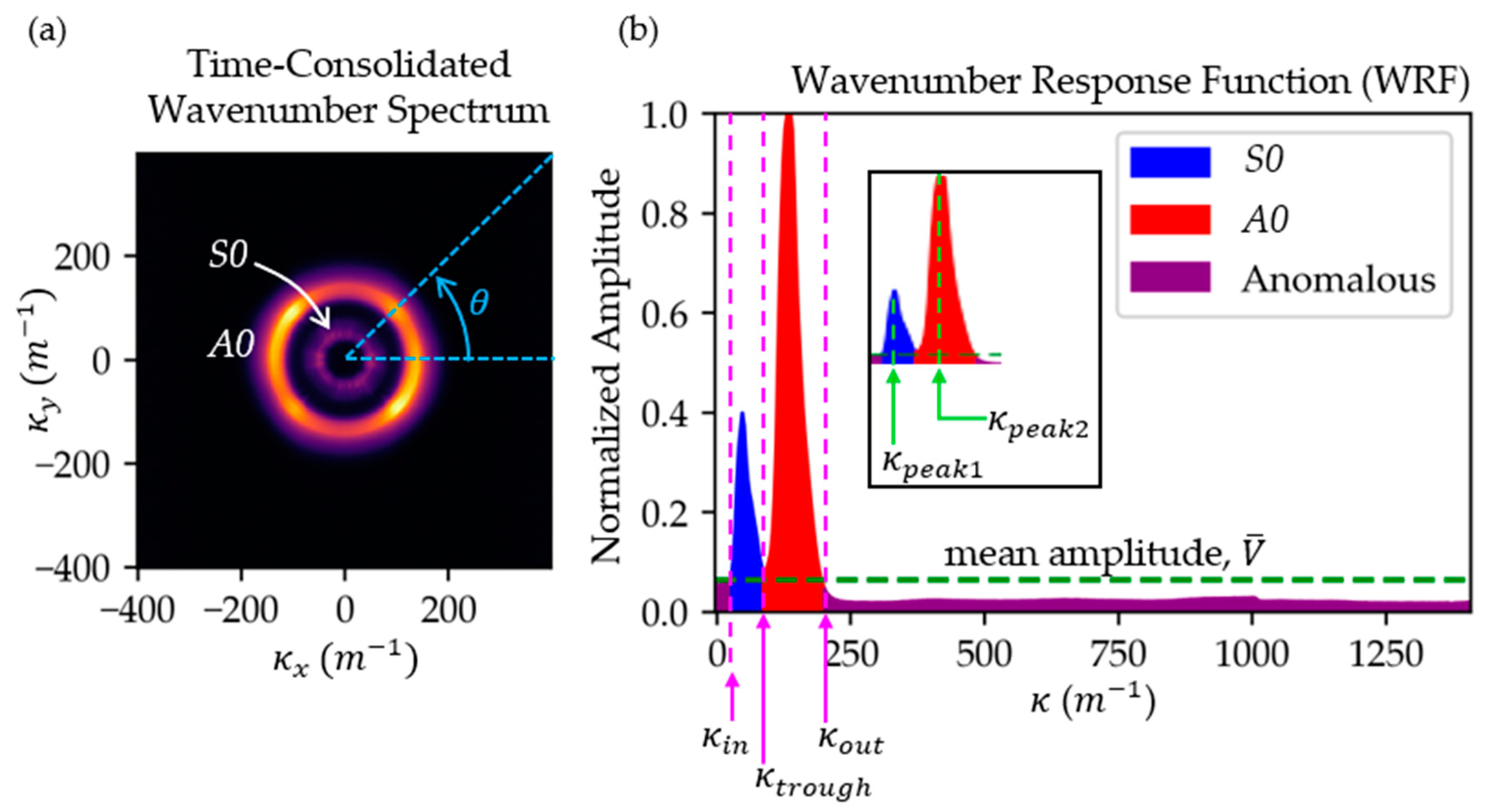
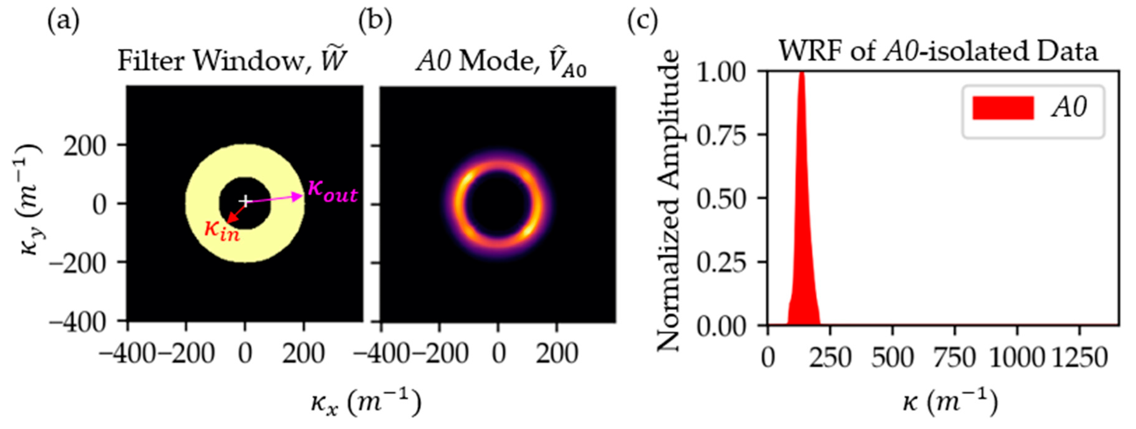
2. Adaptive Mode Filter

In this work, an adaptive mode filter is proposed to isolate a specific mode of interest, so that further analysis or processing for damage visualization can be performed. Figure 1 depicts a typical process flow. Before mode isolation, the measured wavefield dataset undergoes several pre-processing steps, namely the frequency bandpass, DC removal, and Tukey windowing. The frequency bandpass is used to remove noises such as environmental vibration and sampling aliasing; DC removal is used to remove the amplitude shift; and Tukey windowing is used to reduce the spectral leakage in Fourier transformation. The pre-processed data would then be fed into the proposed mode filter to isolate the S0, A0, and the damage-related anomalous modes.
Throughout this paper, x , y , t , f , κ x , κ y , and W represent the x coordinate, y coordinate, time index, frequency index, x direction wavenumber, y direction wavenumber, and filter window, respectively. Symbols v and V generally represent the wavefield data in the original space-time domain and Fourier domain, respectively, and they will be accented if they have been modified by any important signal processing step.
Figure 2 shows the process flow of the proposed adaptive mode filter. The pre-processed space-time domain data v x , y , t will first be converted into the wavenumber-time domain using a 2D FT. The wavenumber-time domain dataset V κ x , κ y , t will be consolidated (i.e., summed) along the time axis into a time-consolidated wavenumber spectrum (TCWS) V ^ κ x , κ y according to
V ^ κ x , κ y = t = 0 T V κ x , κ y , t ,
where the sampling time is indexed by t from 0 to T . Figure 3a shows the amplitude plot of a TCWS, generated using the wavefield data of a 2 mm stainless-steel plate (see Section 3.2 Case P1). Note that the full range of the respective wavenumber scale is ±1000 m−1. This figure only shows the zoom-in view of the meaningful ±400 m−1 range. In this plot, the consolidated energy of the S0 and A0 mode can be identified over the black background as two concentric rings, i.e., S0 as the inner ring and A0 as the outer ring. Following this, a polar coordinate system is employed and an angular-consolidated wavenumber response function (WRF) V ˇ κ is generated as
V ˇ κ = θ = 0 2 π V ^ κ , θ ,
where κ = κ x 2 + κ y 2 and θ represents the angle of consolidation. The WRF is shown in Figure 3b, with the κ ranging up to 1414 m−1 due to its Pythagorean definition. Two prominent peaks which represent the accumulated energy of the S0 and A0 modes can be identified in the WRF. The shorter peak in blue corresponds to the S0 mode that has lower energy, whereas the higher peak in red corresponds to the A0 mode that has higher energy.
Many of the processing steps shown in Figure 2 can easily be graphically understood based on Figure 3b. The κ p e a k 1 and κ p e a k 2 corresponding to the κ value at the peaks of the S0 and A0 modes, respectively, as shown in the inset in Figure 3b, must be found first. Then, the κ t r o u g h can be determined as the κ value at the trough between κ p e a k 1 and κ p e a k 2 . Subsequently, the values of κ i n and κ o u t can be determined as the intersections of the mean amplitude V and the WRF. Note that the mean amplitude of the WRF, denoted as V , is shown in Figure 3b by the dashed horizontal line. All these κ values can be automatically determined using a generic peak-finding algorithm or logical program. Thus, in general, the proposed mode filter can be regarded as a searching procedure using the WRF that automatically enables the identification of κ i n , κ o u t , and κ t r o u g h without any user input for the generation of suitable mode filters.
Once the values of κ i n , κ o u t , and κ t r o u g h are determined, three binary (pass or block) filter windows can be generated for the isolation of S0, A0, and anomalous modes, respectively, as
W ~ S 0 κ x , κ y = 1 , κ i n < κ < κ t r o u g h 0 , otherwise ;
W ~ A 0 κ x , κ y = 1 , κ t r o u g h κ < κ o u t 0 , otherwise ;
W ~ A n o m κ x , κ y = 1 W ~ S 0 κ x , κ y W ~ A 0 κ x , κ y .
The filter window for the A0 mode is shown in Figure 4a, in which the yellow region has unity value (pass), while the black region has a null value (block). The filter window can then be applied to the wavenumber-time domain data as an inner product to isolate the mode such that
V ~ m o d e κ x , κ y , t = W ~ m o d e . V κ x , κ y , t ,
where V ~ m o d e represents the single-mode-filtered wavefield data. Figure 4b shows a sample TCWS of V ~ A 0 based upon its corresponding unfiltered TCWS as previously shown in Figure 3a. Figure 4c shows the corresponding A0-isolated WRF. From a number of attempts made by the authors, it was found that even though the data consolidation results in TCWS and WRF of different shapes and amplitudes, the filter windows can be employed to isolate the modes effectively. In other words, the adaptability of the proposed mode filter is anchored at the representation of wavefield data using the WRF.
Although only one sample solution of the isolated mode is presented in Figure 3 and Figure 4, the proposed mode filter can actually generate all three S0-isolated, A0-isolated, and anomalous mode-isolated wavefield data in one execution of the algorithm. The anomalous mode will contain energy only when a portion of energy from the incident modes is mode-converted by a damage.

3. Experimental Investigation

The proposed adaptive mode filter was experimentally investigated for its ability to isolate a mode and subsequently improve the clarity of the damage visualization using a pristine (i.e., damage-free) specimen and four specimens with artificial damages, respectively. The details of the data acquisition setup, specimens, and result visualization methods are given in the following sub-sections.

3.1. Data Acquisition System

A set of laser-scanning G-UPI system was used for the actuation and measurement of Lamb waves in the specimens. For actuation, a diode-pumped solid-state Q-switched pulsed laser (custom-made by Advanced Optowave Inc., Ronkonkoma, NY, USA) with a wavelength of 532 nm, a beam diameter of approximately 4 mm, a pulse width of approximately 40 ns, pulse energy of approximately 1.5 mJ, and pulse repetition frequency of 50 Hz was used as the ultrasound generator. Note that the laser parameter values were set to ensure ultrasound generation within the non-destructive, linear thermoelastic regime of all specimens without any ablation. Rectilinear grid-point scanning was realized using a galvano-motorized laser mirror scanner (ScanCube7, ScanLab GmbH, Puchheim, Germany) with a scan interval (i.e., spatial sampling resolution) of 0.5 mm in both the horizontal x and vertical y directions.
For measurement, an amplifier-integrated PZT (lead zirconate titanate) sensor (M304-A, Fuji Ceramics Corp., Fujinomiya, Japan) was used. It has a broad frequency bandwidth up to 1 MHz and a sensitivity of 110–115 dB in the frequency range of 160–350 kHz, with reference to 0 dB at 1 V/ms−1. It was bonded on the specimen using a cyanoacrylate adhesive, either on the same side of the laser-scanning surface similar to a standard NDT inspection, or on the opposite side similar to the inspection of a smart (instrumented) structure. The sensor converts the surface displacement of the specimen into analogue electrical signals. The analogue signals were filtered using a variable cut-off frequency filter (3627, NF Corp., Yokohama, Japan) by manually sweeping the bandpass frequency until a suitable range was found, where there were two distinct modes and the signal-to-noise ratio was sufficient. This was performed without any investigation into the correlation with the rate of damage detection. Each signal was digitized into 500 samples using an 8-bit oscilloscope (USB-5133, National Instrument Corp., Austin, TX, USA). Note that the actuation-measurement process was performed consecutively one after another, until the signals from all scanning grid points were saved as a 3D space-time wavefield data v ( x , y , t ) .

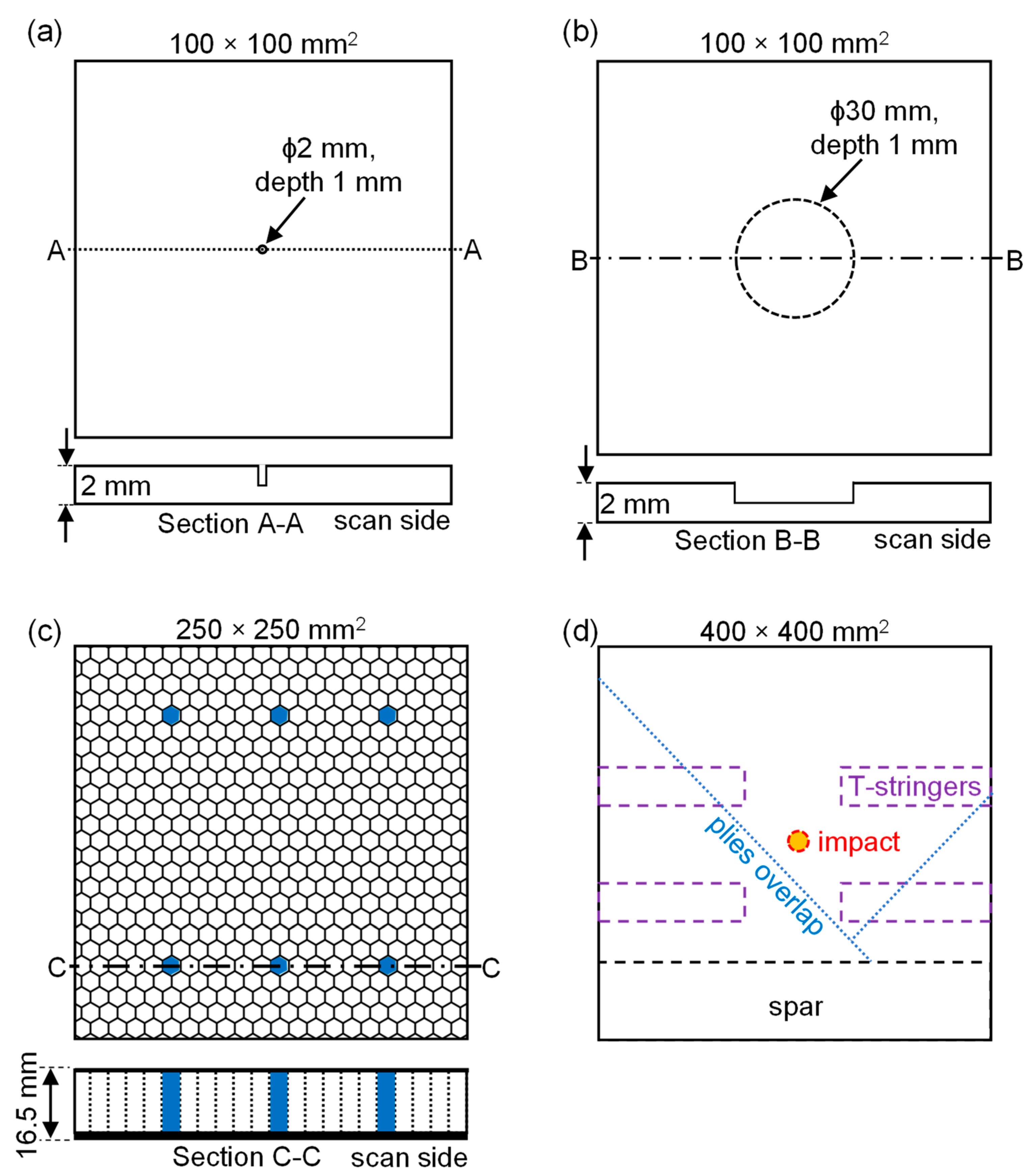
3.2. Specimen and Inspection Setup

For the verification of mode-isolation effectiveness, inspection Case P1 (Pristine 1) was performed using a pristine stainless-steel plate. Unless specified otherwise, the wavefield was measured from an imaging region of interest (ROI) that was located at the centre of specimen, and the origin was located at the lower left corner of the ROI. The specimen information and inspection parameters for all cases are summarized in Table 1. The save data were further software filtered using various frequency bandpasses to verify the effectiveness of the proposed mode filter regardless of the frequency bandwidth.
Improved damage visualization based on mode-isolated data was demonstrated using four specimens with artificial damage. In the first two cases, a stainless-steel plate was used to represent a simple, homogeneous structure. A blind hole was drilled and a circular area was milled on the opposite side of the specimen, respectively, for Cases D1 and D2, to simulate scatterer-type damage-like cracks and hidden corrosion. The damage diameter was large compared to the ultrasound wavelength in Case D2, so the ultrasound perceived it as areal-type damage, unlike in Case D1. Illustrations of the imaging ROI for all damaged cases are given in Figure 5.
In Case D3, an aluminium-sandwiched panel with a honeycomb core was used as the specimen. The panel had a total thickness of 16.5 mm, with a front facesheet thickness of 1.0 mm, a hexagonal core thickness of 15.0 mm, and a rear facesheet thickness of 0.5 mm. The core had a cell size of 10.4 mm and a wall thickness of 0.05 mm. Six pinholes were drilled at the back of the specimen, and water was injected into the honeycomb cell using a syringe through one of the pinholes while the specimen was placed horizontally. The pinhole was then sealed with cellophane tape to prevent water from escaping, and the specimen was positioned upright for scanning. This process was consecutively repeated for all six pinholes to simulate water ingress damages at different locations.
In Case D4, a previously tested section of a carbon fibre-reinforced plastic (CFRP) wing from [42] was used as the specimen. The overall dimensions of the wing section are unavailable, but its nominal skin thickness is known to be 2.0 mm. The sensor was fixed on the spar web at a linearized distance of approximately 130 mm from the bottom of ROI. This inspection case was chosen to demonstrate the ability of the proposed mode filter to isolate a specific mode of interest for further structural imaging of complex structures.

3.3. Result Visualization

The 3D space-time wavefield data v ( x , y , t ) must be processed into images for damage visualization and performance analysis. Two result processing methods used in this study are briefly described in the following sub-sections.

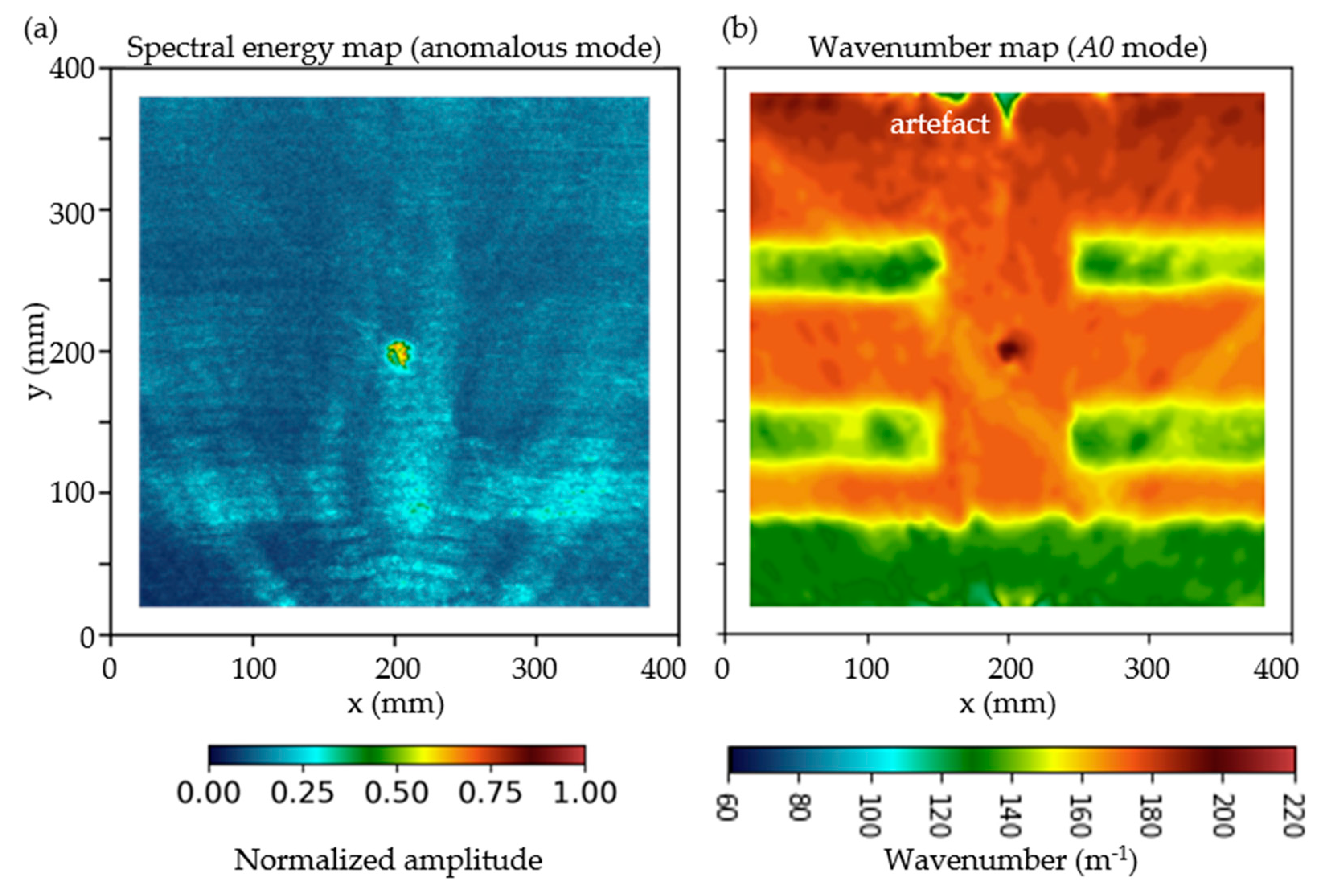
3.3.1. Spectral Energy Mapping

Spectral energy mapping is proposed in this work as an alternative to the accumulated mass-normalized kinetic energy mapping [47,48] and Hilbert-enveloped energy mapping [47] for visualizing damage, as it provides higher contrast. However, a thorough investigation of its characteristics is beyond the scope of this work and remains to be performed. To generate a spectral energy map (SEM), the space-time wavefield data v ( x , y , t ) , regardless of the mode filtering status, is transformed into the space-frequency domain as V ( x , y , f ) using a 1D FT and then summed along the frequency axis, such that
SEM ( x , y ) = f = 1 n V x , y , f .

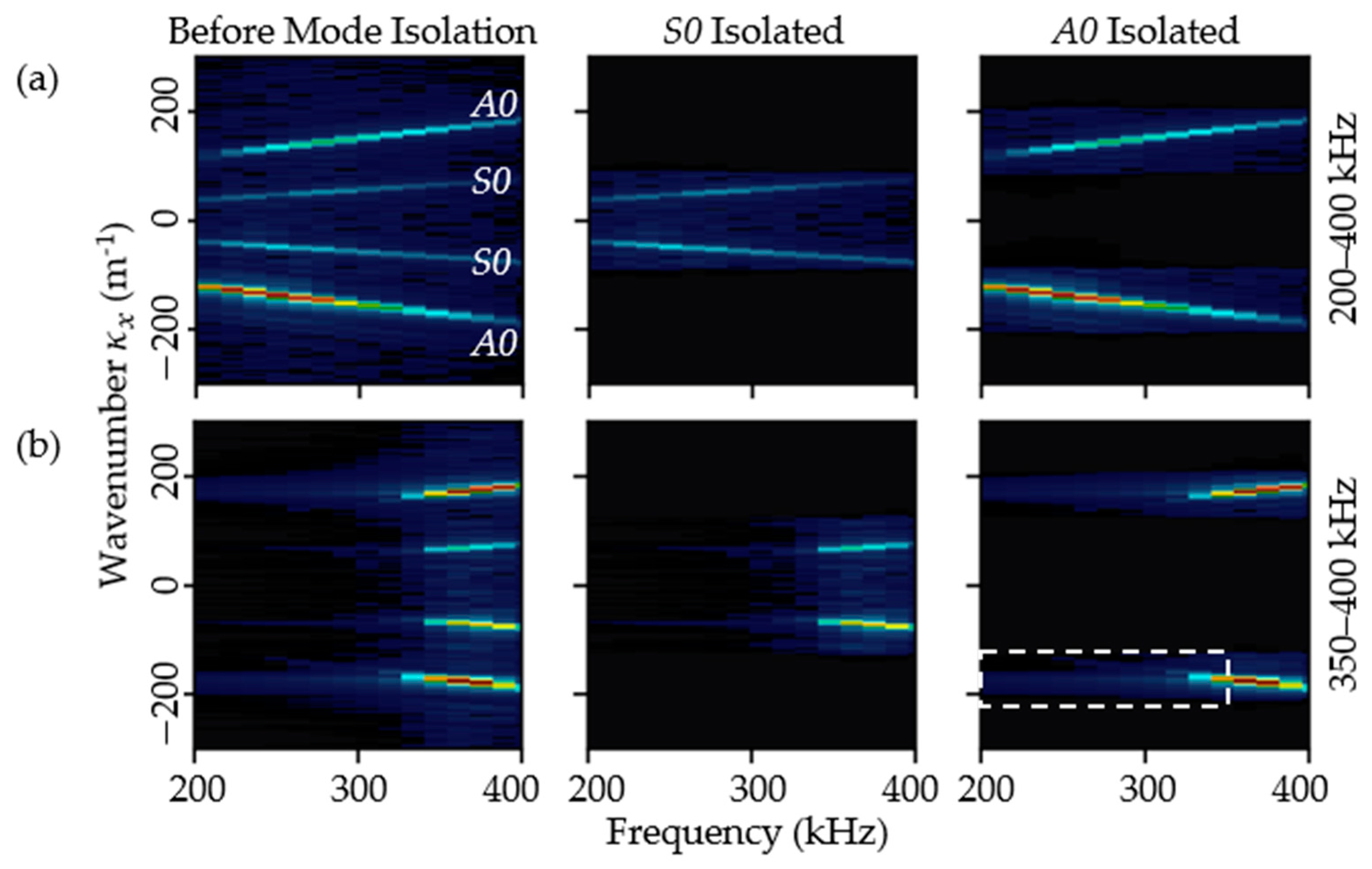
3.3.2. Wavenumber Imaging

Wavenumber imaging is a result processing method that processes wavefield data into a wavenumber map. The wavenumber map in this context refers to an image that displays the distribution of the local wavenumber value of an inspected specimen. There are several variants and the one reported in [42] was adopted after replacing its original mode filter with the one proposed in this paper.

3.4. Performance Metric

In order to quantify the efficiency of mode filtering, a performance metric hereby called the energy ratio (ER) was proposed as
E R = t 1 t 2 A a f t e r 2 t 1 t 2 A b e f o r e 2 × 100 % ,
where symbol A represents the signal envelope of a mode before or after mode filter processing. The envelope is calculated for the entire time signal using Hilbert transformation, while the time window for summation is determined on a case-by-case basis, as indicated by the yellow and pink time zones in Figure 6. The square value was used for the sake of matching the definition of kinetic energy per unit mass. No further calibration was performed and it can be used without losing its genericity. The ER delivers a positive value which represents the ratio of energy remaining in a specific mode compared to its energy before mode filter processing. The value approaching 0% represents a good performance for the suppression of an unwanted mode, while a value near 100% represents good performance for the isolation of a desired mode. Note that ER values above 100% are possible, for example, when the mode isolation removes the destructive interference of original modes.

4. Results and Discussions

This section is divided into two sub-sections. Section 4.1 presents the verification of mode filtering effectiveness. Section 4.2 provides evidences that the proposed mode filter can produce single-mode data not only for the visualization of hidden damage with improved clarity, but also critically needed for the structural imaging of complex thin-walled structures.

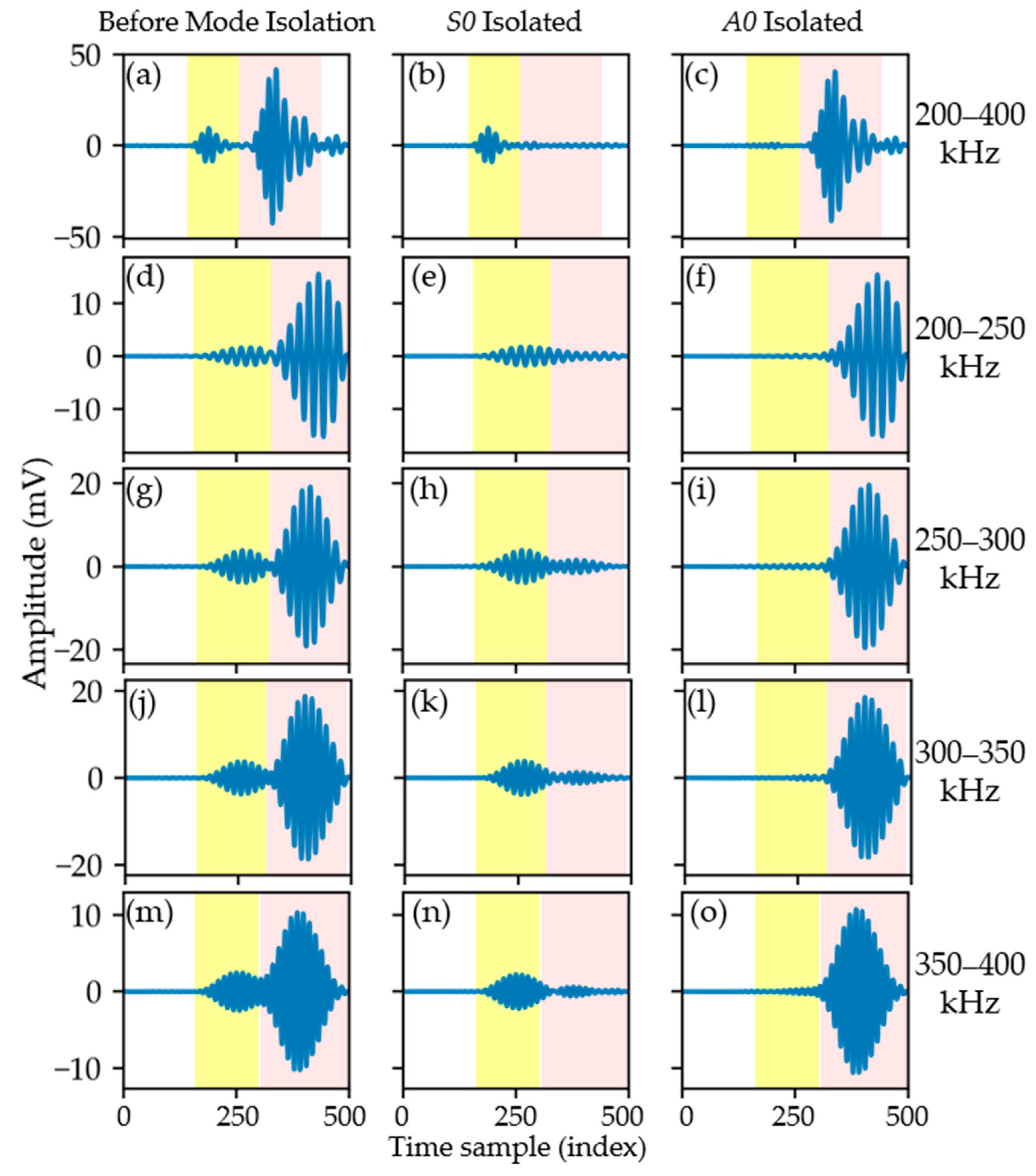
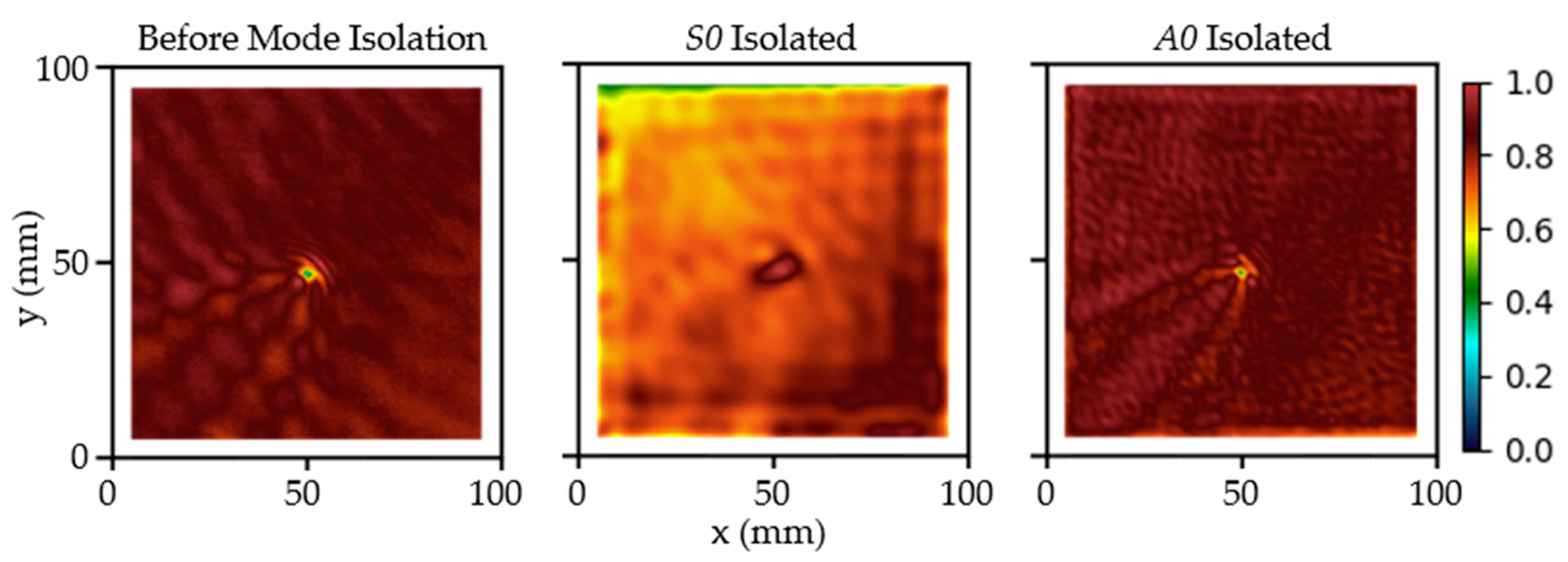
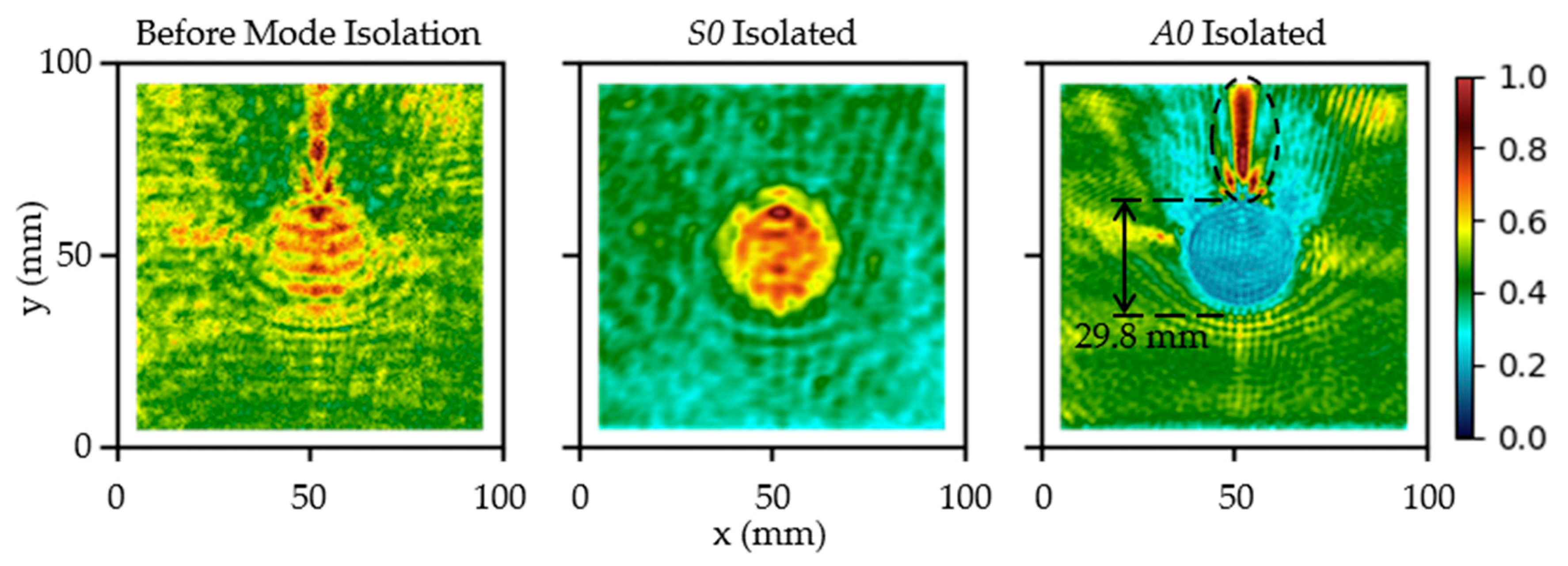
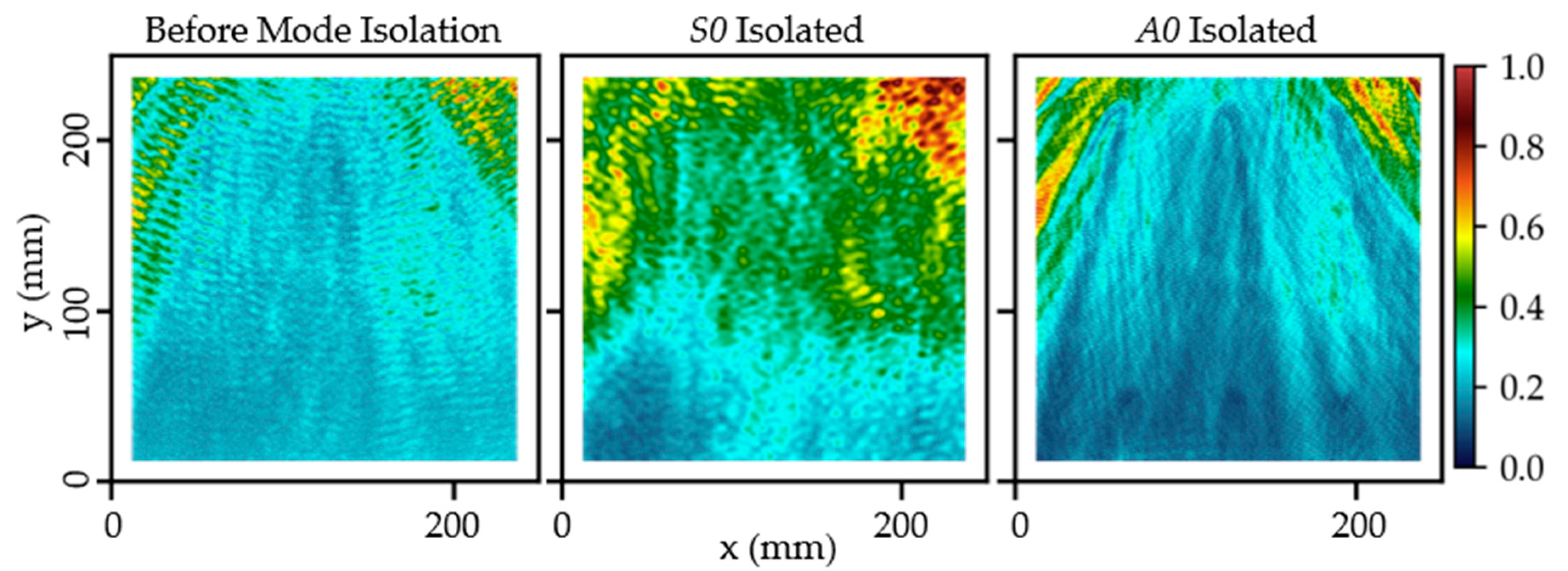
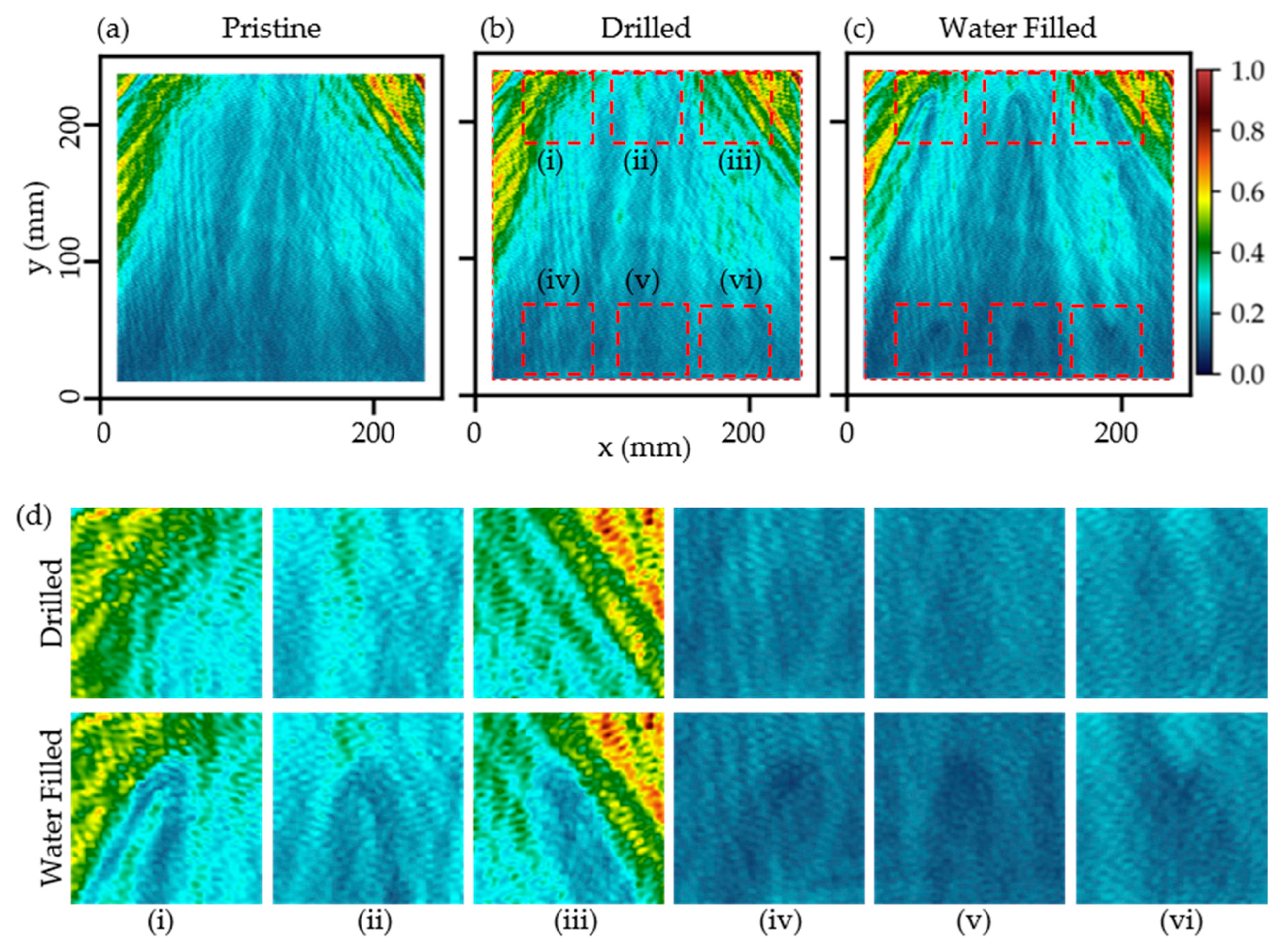
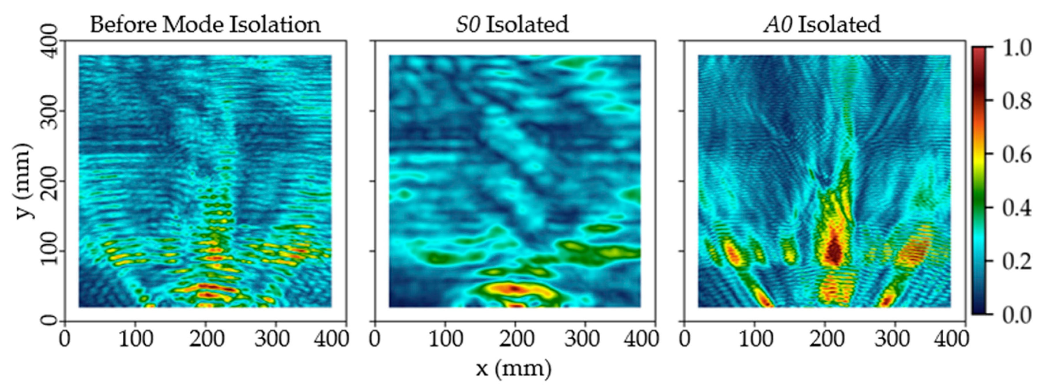
4.1. Effectiveness of Mode Filtering

The effectiveness of the proposed mode filter was verified using the wavefield data acquired from inspection Case P1. An example of time-domain signal of the wavefield is shown in Figure 6a. Note that these data have a wide frequency bandwidth of 200–400 kHz, as acquired during the experiment. The left, middle, and right columns of Figure 6 show the signals before applying the mode filter, after S0 mode isolation, and after A0 mode isolation, respectively. All sub-figures share the same horizontal axis, which was given as a time-sample index for easier reference. The vertical axis shows the signal amplitude in millivolts without losing its genericity to represent the linear-elastic surface displacement of the specimen. As shown in Figure 6a, the signal before mode filtering contains two distinctive modes. This agrees well with the theoretical dispersion curves of the 2 mm stainless-steel specimen plate given in Figure 7, which was generated using the Vallen Dispersion software [49]. The dispersion curves clearly show that the specimen can only support two wave modes, i.e., the S0 and A0 modes for the frequency range 200–400 kHz used in the experiment. Additionally, the group velocity of the S0 mode is higher than that of the A0 mode throughout the frequency range, which allows the identification of the first mode (yellow background) in Figure 6a as the S0 mode, and the second (pink background) as the A0 mode.
The effectiveness of the mode filter to isolate a specific mode of interest is seen to be excellent by inspecting the middle and right columns of Figure 6. When the mode filter was applied to isolate the S0 mode, as shown in Figure 6b, the S0 mode could be seen to be well preserved with neither mode distortion nor significant amplitude loss. At the same time, the A0 mode could be seen to be effectively removed with only a little residue. The mode filter exhibits a similar effectiveness for the isolation of the A0 mode. When the mode of interest is the A0 mode, the A0 mode could be isolated without any detectable mode distortion or amplitude lost, as shown in Figure 6c. This result qualitatively demonstrates that the proposed mode filter can effectively isolate a specific mode of interest from wavefield data which have a broad frequency bandwidth.
The energy ratios (ER) for the signals before and after mode isolation were calculated to quantitatively scrutinize the filter effectiveness. Specifically for S0 mode isolation, the energy of the S0 mode before mode isolation, corresponding to the time zone between indexes 142 and 260, as indicated with a yellow background in Figure 6a, was compared to the energy of S0 mode after mode isolation, corresponding to the same time zone (yellow) in Figure 6b. The ER was found as 101.3%, indicating an effective isolation of S0 mode with a negligible energy gain. The isolation of the S0 mode is only meaningful if the A0 mode is effectively suppressed. The ER corresponding to the A0 mode suppression was calculated based on the energy of the A0 mode before mode isolation, corresponding to the time zone between indexes 260 and 441, as indicated by the pink background in Figure 6a, compared to the energy of the A0 mode after mode isolation, corresponding to the same time zone (pink) in Figure 6c. It was found that ER = 0.1% indicates an excellent suppression of the A0 mode. Using the same ER analysis, the effectiveness of the A0 mode isolation and S0 mode suppression was found to be 96.0% and 1.3%, respectively. This ER analysis quantitatively proved that the proposed mode filter can effectively isolate a specific mode of interest and at the same time suppress other irrelevant modes, even though the wavefield data have a broad frequency bandwidth.
The signals shown in Figure 6a–c have a frequency bandwidth of 200–400 kHz, which represents a typical broadband data bandwidth. However, for wavefield acquisition using the scanning sensing scheme (see the wavefield acquisition scheme in [19]), the wavefield is often excited using a contact transducer at a much narrower frequency bandwidth. In order to show the adaptability of the mode filter for narrow band wavefield data, the broadband wavefield acquired for Case P1 was further software-filtered into a few narrow frequency bandwidths at 200–250 kHz, 250–300 kHz, 300–350 kHz, and 350–400 kHz, as shown in Figure 6d–o. When the A0 mode is of interest, the A0 mode can be effectively isolated without any mode distortion or amplitude reduction, as shown within the pink time zone in Figure 6f,i,l,o. The same sub-figures also show that the S0 mode was effectively suppressed until its existence could not be identified within the yellow time zones. On the other hand, when the S0 mode is of interest, the S0 mode can effectively be isolated without any visible amplitude reduction, as shown within the yellow time zone in Figure 6e,h,k,n. However, visible residues of the A0 mode exists within the pink time zones in the same sub-figures. Further discussion regarding the residual will be given at the end of this sub-section.
The ER of all cases were calculated and summarized in Table 2 for quantitative analysis. When isolating the S0 mode, the ER for the S0 mode is higher than 100%, indicating an excellent mode isolation, except for bandpass 350–400 kHz, which has an ER = 78.2%. This low ER was probably caused by the merging of the S0 and A0 modes in the time domain, as shown in Figure 6m, which prevented the accurate calculation of the mode energy for the realistic representation of the filter efficiency. At the same time, excellent efficiency was recorded for the suppression of the A0 mode, as indicated by the ER ranges between 0.1% and 0.8%. On the other hand, when isolating the A0 mode, the ER for the A0 mode was found to be close to 100%—between 96.0% and 106.9%—indicating a superb A0 isolation efficiency. At the same time, the suppression of the S0 mode was also found to be effective by the ER ranges between 1.3% and 4.5%. Such high efficiency would be sufficient for further damage visualization or analysis using either the isolated S0 or A0 mode, which will be further discussed in the next sub-section. This simple analysis of the time-domain signals proved that the proposed mode filter can effectively isolate a mode of interest and suppress an unwanted mode for the wavefield of the broad frequency band as well as for the wavefield of the relatively narrow frequency band.
The efficiency of the mode filter can also be inspected in the wavenumber-frequency domain. By converting the wavefield data into the wavenumber-frequency domain using 3D FT, the modes can be compressed into respective dispersion curves. This provides a convenient avenue to check whether the partially overlapped S0 and A0 modes in the time domain, as shown in Figure 6m, was completely separated by the mode filter in the wavenumber-frequency domain. Figure 8a,b show the wavenumber-frequency spectrums at κ y = 0 for wavefield data in the 200–400 kHz and 350–400 kHz frequency bands, respectively. The spectrum before mode isolation in Figure 8a shows the distribution of energy over the wavenumber-frequency domain, in which the S0 mode can be seen to form two curves that are located closer to the horizontal axis κ x = 0 m 1 , while the A0 mode formed the top and bottom curves. The energy content of the A0 mode is comparatively higher than the S0 mode, consistent with that shown in Figure 6a. A complete separation of modes can be seen in the middle and right spectrums of Figure 8a after applying the mode filter. Figure 8b shows the spectrum corresponding to the time-domain signal shown in Figure 6m,n,o. The partial overlap of the S0 mode and A0 mode in the time domain is not seen in the wavenumber-frequency domain. This simply proved that the residual of the A0 mode within the pink time zone in Figure 6e,h,k,n was not caused by the inefficiency of the proposed mode filter. Instead, close examination of the spectrums shows that there were energy leakages during the frequency bandpass, as indicated by non-zero energy distribution within the white dashed box in Figure 8b. Note that the box spans frequencies from 200 kHz to 350 kHz and should contain no energy if the frequency bandpass was performed without leakage. How the energy leakage in the frequency domain affected the time domain signal and how the software bandpass could be configured to reduce or mitigate energy leakage are subjected to further investigation beyond the scope of this paper.

4.2. Advantages of the Mode Filter

This sub-section presents the advantages of the proposed mode filter for clearer damage visualization and the structural imaging of complex thin-walled structures. Inspection Case D1 was performed to visualize a point-like damage. The unfiltered, S0-isolated, and A0-isolated data were processed as spectral energy maps (SEMs), as shown in Figure 9. A 5% crop was applied to four edges of all SEMs to remove any processing artefacts due to the boundary effects. The damage could actually clearly be seen without any mode filtering, so the improvement in clarity using the mode filter can hardly be perceived. Anyway, this result shows that the clarity of damage visualization is indeed dependent on the mode of selection, evident by a distorted visualization of damage using the S0-isolated data, in contrast to the accurate visualization of the same damage using the A0-isolated data.
Inspection Case D2 was performed to show that the mode-filtered data can also be used to improve the clarity of damage visualization for areal-type damage. The unfiltered, S0-isolated, and A0-isolated data were processed as SEMs, as shown in Figure 10. The corrosion damage could be seen in the SEMs processed from the data before applying the mode filter, but it is difficult to identify its actual shape and size. After isolating the S0 mode using the mode filter, the corrosion damage could be clearly identified. The resolution of this image is good enough to facilitate the damage size measurement. When the A0-isolated data were used, the SEM show a much clearer damage boundary due to the shorter wavelength of the A0 mode. The size of the damage can be accurately measured from the SEM as 29.8 mm, which is in excellent agreement with the actual damage size. An interesting feature above the damage, as indicated by a dashed oval, was caused by the focusing effect of the damage. In this particular case, the damage acted as an acoustic lens [50,51] and focused much of the wave energy towards the top of SEM.
Inspection Case D3 was performed to show that the proposed mode filter is highly adaptive to different specimens and types of damage. The unfiltered, S0-isolated, and A0-isolated data were again processed as SEMs, as shown in Figure 11. The energy distribution appeared more complicated compared to that of the isotropic specimens used in Cases D1 and D2. This was due to the existence of additional reflections and scatterings at all facesheet-cell wall interfaces, on top of the incident S0 and A0 modes. In addition, the cell walls create directional energy dispersion [39,52] and non-isotropic wave behaviour [53,54], causing inconsistent energy distribution over the SEM. As a result of wave interferences and uneven energy distribution, the six honeycomb cells that were filled with water as artificial water ingress damage cannot be identified at all in Figure 11 before mode isolation. They cannot also be identified after the isolation of the S0 mode, most probably due to the low resolution associated with the long wavelength of the S0 mode. Some traces of energy change can be identified when the A0-isolated data were used. This is consistent with the literature on A0 mode providing a better resolution for higher-image clarity [55,56]. The water-filled cells were perceived by the wavefield as energy absorbers, which can be identified in the SEM as cone-shaped wakes pointing towards the wavefield source that was located far above the inspection ROI, i.e., at (125, 375) mm.
In order to have easier damage identification, the SEM processed from the A0-isolated data at the pristine (as manufactured) state, after the drilling of six water-injecting holes on the opposite side of the specimen, and after the cells were filled with water, were generated for comparison, as shown in Figure 12a–c, respectively. The nearly identical Figure 12a,b prove that the drilling of six water-injecting holes at the opposite side of the specimen did not alter the energy distribution of the wavefield. The energy distribution was disturbed only after water was injected into the selected cells, which can be seen by comparing Figure 12b,c. Six small regions around the water-filled cells, indicated by red dashed boxes (i)–(vi), were enlarged and given in Figure 12d for easier comparisons. The three water-filled cells within regions (i)–(iii) are more apparent in the enlarged SEM, in which the wake pattern as well as the reduction in energy can be seen. The other three water-filled cells within regions (iv)–(vi) are hard to identify due to the low availability wavefield energy at the bottom of the ROI. In this case, the source of the wavefield was located far above the inspection ROI, i.e., at (125, 375) mm. Almost all the wavefield energy was dissipated or directed to the left and right sides of the specimen (beyond the inspection ROI) due to the wave-guiding nature of the honeycomb core [39,52]. The remaining energy reaching the three water-filled cells at the bottom cannot create sufficient contrast for visualization.
Inspection Case D4 was performed to show that the proposed mode filter supports clear damage visualization and structural imaging for complex thin-walled structures. The SEMs for unfiltered, S0-isolated, and A0-isolated data are given in Figure 13. The complex energy distribution in SEMs, caused by the intricate interactions of incident waves, scattering, reflection, and mode-converted waves from both benign structural components and damage prevents the identification of damage, in contrast to previous inspections.
The adaptability of the mode filter for complex structure inspection can be demonstrated by removing all incident modes when necessary. When all incident modes, including those related to benign structural components, were removed, the wavefield data only contained a damage-induced anomalous mode, which is denoted as v ~ A n o m x , y , t as given previously in Figure 1. The filtered data can also be processed as SEM, as shown in Figure 14a. In this case, the SEM shows high-energy distribution at the damaged region, and thus highlights the damage for easy detection. At the same time, the energies of all waves related to benign structural components were suppressed, until the structural components can barely be visualized. To prove that the proposed mode filter also facilitates the mode isolation for structural imaging, the A0-isolated data v ~ A 0 x , y , t , also previously shown in Figure 1, was processed using the modified wavenumber imaging algorithm (see Section 3.3.2) as a wavenumber map, as shown in Figure 14b. In this wavenumber map, the spar flange is shown in green, correspond to a wavenumber value of approximately 130 m−1; the four stringers are shown in greenish-yellow (~145 m−1); the ply overlapped regions are shown in yellowish-orange (~167 m−1); and the nominal 2 mm skin is shown in orange (~173 m−1). The impact damage, which can be identified at the centre of the image, is shown in maroon (~196 m−1). The artefact that is most probably due to non-optimum parameter settings in the wavenumber imaging can be seen at the top, subjected to further investigation. Note that the wavenumber value is a physical value of the specimen, which can be converted to specimen thickness if necessary [57,58]. The significant improvement in damage visibility by comparing Figure 13 and Figure 14a proves that the proposed mode filter has an excellent adaptability for simple specimens and complex structures. Figure 14 also proves that the proposed mode filter is highly adaptive for isotopic metallic specimens and anisotropic composite structures.

5. Concluding Remarks

We propose an adaptive mode filter to overcome the signal processing difficulties encountered in guided ultrasonic waves propagation imaging (G-UPI) of aerospace thin-walled structures. The interference of dispersive multimodal Lamb waves makes it challenging to isolate a mode of interest consistently using conventional methods, which require ad hoc or manual optimizations. Our approach compresses the wavefield into a wavenumber response function (WRF) to generate a suitable wavenumber filter mask without subjective optimization. The filter mask is highly adaptive as the WRF reflects differences in signal bandwidth, specimen material, and damage type. Applying the filter mask in the wavenumber-time domain enables the automatic isolation or removal of individual modes for the highlighting of damage or structural imaging. It guarantees consistent results by removing human subjectivity from the processing and it is fast due to the adoption of 2D Fourier transform (FT) instead of 3D FT.
The effectiveness of the proposed mode filter was tested and proven in experiment Case P1 through analysis in the time and wavenumber-frequency domains. The filter successfully isolated the mode of interest and suppressed unwanted modes with superb effectiveness, which was not affected by the frequency bandwidth of the data. Quantitatively, the filter retained 78.2–122.0% energy of the targeted modes and suppressed unwanted modes to 0.1–4.5%. Four additional inspections were performed to test the adaptability of the proposed mode filter to different materials and types of damage. The inspection of Cases D1 and D2 involved the use of isotropic stainless-steel plates with scatterer-type and areal-type damage, respectively. The inspections of Cases D3 and D4 were conducted on an aluminium honeycomb panel with water ingress and a carbon fibre-reinforced plastic wing section with impact damage, respectively. These structures with anisotropic and complex internal features are more representative of realistic scenarios. All damages were successfully detected and visualized after mode isolation or removal using the proposed mode filter, thus confirming its ability to adapt to various materials and types of damage.
There are several opportunities to expand this work. Firstly, the capability of the filter could be extended to accommodate wavefields with a broader bandwidth, where multiple (>2) modes are present. Secondly, it would be beneficial to investigate the suitability of the filter for highly anisotropic specimens. Furthermore, the filter could be expanded to isolate mode conversion, such as isolating Scholte waves [59] to provide a more accurate evaluation of water ingress in honeycomb sandwich structures.

Author Contributions

Conceptualization, C.C.C.; Methodology, C.C.C.; Software, M.A.A.S.; Validation, C.C.C. and M.Y.H.; Formal Analysis, M.A.A.S.; Investigation, M.A.A.S. and C.C.C.; Resources, M.Y.H., J.-R.L. and H.R.R.; Data Curation, M.A.A.S.; Writing—Original Draft Preparation, C.C.C. and M.A.A.S.; Writing—Review & Editing, M.Y.H., J.-R.L. and H.R.R.; Visualization, M.A.A.S. and C.C.C.; Supervision, M.Y.H., J.-R.L. and H.R.R.; Project Administration, M.Y.H.; Funding Acquisition, M.Y.H. All authors have read and agreed to the published version of the manuscript.

Funding

This research was funded by the Industrial Research Grant Scheme through Endowment of Tan Sri Syed Azman Syed Ibrahim (Account Vote Number: 6338201-10801).

Data Availability Statement

Not applicable.

Acknowledgments

The authors acknowledge the support from the Universiti Putra Malaysia and by the Industrial Research Grant Scheme through Endowment Tan Sri Syed Azman Syed Ibrahim (Account Vote Number: 6338201-10801). The authors also acknowledge the support by the Brain Pool program funded by the Ministry of Science and ICT through the National Research Foundation of Korea (2021H1D3A2A01100011).

Conflicts of Interest

The authors declare no conflict of interest.

References

  1. Arena, M.; Ambrogiani, P.; Raiola, V.; Bocchetto, F.; Tirelli, T.; Castaldo, M. Design and Qualification of an Additively Manufactured Manifold for Aircraft Landing Gears Applications. Aerospace 2023, 10, 69. [Google Scholar] [CrossRef]
  2. Kim, M.; Kim, Y. A Thermo-Mechanical Properties Evaluation of Multi-Directional Carbon/Carbon Composite Materials in Aerospace Applications. Aerospace 2022, 9, 461. [Google Scholar] [CrossRef]
  3. Rajak, D.K.; Wagh, P.H.; Kumar, A.; Sanjay, M.R.; Siengchin, S.; Khan, A.; Asiri, A.M.; Naresh, K.; Velmurugan, R.; Gupta, N.K. Impact of fiber reinforced polymer composites on structural joints of tubular sections: A review. Thin-Walled Struct. 2022, 180, 109967. [Google Scholar] [CrossRef]
  4. Cui, Z.; Wang, Z.; Cao, F. Research on Mechanical Properties of V-Type Folded Core Sandwich Structures. Aerospace 2022, 9, 398. [Google Scholar] [CrossRef]
  5. Zhou, J.; Liu, B.; Wang, S. Finite element analysis on impact response and damage mechanism of composite laminates under single and repeated low-velocity impact. Aerosp. Sci. Technol. 2022, 129, 107810. [Google Scholar] [CrossRef]
  6. Othman, M.S.; Chun, O.T.; Harmin, M.Y.; Romli, F.I. Aeroelastic effects of a simple rectangular wing-box model with varying rib orientations. IOP Conf. Ser. Mater. Sci. Eng. 2016, 152, 012009. [Google Scholar] [CrossRef]
  7. Chan, Y.N.; Harmin, M.Y.; Othman, M.S. Parametric study of varying ribs orientation and sweep angle of un-tapered wing box model. Int. J. Eng. Technol. 2018, 7, 155–159. [Google Scholar] [CrossRef]
  8. Dawood Al-Wasiti, S.D.S.; Harmin, M.Y.; Harithuddin, A.S.M.; Chia, C.C.; Rafie, A.S.M. Computational Study of Mass Reduction of a Conceptual Microsatellite Structural Subassembly Utilizing Metal Perforations. J. Aeronaut. Astronaut. Aviat. 2021, 53, 57–66. [Google Scholar]
  9. Dawood, S.D.S.; Harithuddin, A.S.M.; Harmin, M.Y. Modal Analysis of Conceptual Microsatellite Design Employing Perforated Structural Components for Mass Reduction. Aerospace 2022, 9, 23. [Google Scholar] [CrossRef]
  10. Bin Kamarudin, M.N.; Mohamed Ali, J.S.; Aabid, A.; Ibrahim, Y.E. Buckling Analysis of a Thin-Walled Structure Using Finite Element Method and Design of Experiments. Aerospace 2022, 9, 541. [Google Scholar] [CrossRef]
  11. Shao, Z.; Zhang, C.; Li, Y.; Shen, H.; Zhang, D.; Yu, X.; Zhang, Y. A Review of Non-Destructive Evaluation (NDE) Techniques for Residual Stress Profiling of Metallic Components in Aircraft Engines. Aerospace 2022, 9, 534. [Google Scholar] [CrossRef]
  12. An, J.H.; Din, S.; Ahmed, H.; Lee, J.R. Simultaneous external and internal inspection of a cylindrical CFRP lattice-skin structure based on rotational ultrasonic propagation imaging and laser displacement sensing. Compos. Struct. 2021, 276, 114592. [Google Scholar] [CrossRef]
  13. Ahmed, O.; Wang, X.; Tran, M.-V.; Ismadi, M.-Z. Advancements in fiber-reinforced polymer composite materials damage detection methods: Towards achieving energy-efficient SHM systems. Compos. Part B Eng. 2021, 223, 109136. [Google Scholar] [CrossRef]
  14. Balageas, D. Introduction to Structural Health Monitoring. In Structural Health Monitoring; ISTE Ltd.: London, UK, 2006; p. 495. [Google Scholar]
  15. Fomitchov, P.A.; Kromin, A.K.; Krishnaswamy, S.; Achenbach, J.D. Imaging of damage in sandwich composite structures using a scanning laser source technique. Compos. Part B Eng. 2004, 35, 557–562. [Google Scholar] [CrossRef]
  16. Ostachowicz, W.; Kudela, P.; Radzienski, M. Guided Wavefield Images Filtering for Damage Localization. Key Eng. Mater. 2013, 558, 92–98. [Google Scholar] [CrossRef]
  17. Chia, C.-C.; Jang, S.-G.; Lee, J.-R.; Yoon, D.-J. Structural damage identification based on laser ultrasonic propagation imaging technology. In Optical Measurement Systems for Industrial Inspection VI; International Society for Optics and Photonics Location: Bellingham, WA, USA, 2009; Volume 7389, p. 73891S. [Google Scholar]
  18. Moore, P.O.; Workman, G.L. Nondestructive Testing Overview; The American Society for Nondestructive Testing: Columbus, OH, USA, 2012; Volume 10. [Google Scholar]
  19. Chia, C.C.; Lee, S.Y.; Harmin, M.Y.; Choi, Y.; Lee, J.-R. Guided Ultrasonic Waves Propagation Imaging: A Review. Meas. Sci. Technol. 2023, 34, 052001. [Google Scholar] [CrossRef]
  20. Rose, J.L. Ultrasonic Guided Waves in Solid Media; Cambridge University Press: Cambridge, UK, 2014. [Google Scholar]
  21. Lamb, H. On Waves in an Elastic Plate. Proc. R. Soc. Lond. Ser. A Contain. Pap. A Math. Phys. Character 1917, 93, 114–128. [Google Scholar]
  22. Sharma, V.K.; Hanagud, S.; Ruzzene, M. Damage Index Estimation in Beams and Plates Using Laser Vibrometry. AIAA J. 2006, 44, 919–923. [Google Scholar] [CrossRef]
  23. Kudela, P.; Ostachowicz, W.; Żak, A. Damage detection in composite plates with embedded PZT transducers. Mech. Syst. Signal Process. 2008, 22, 1327–1335. [Google Scholar] [CrossRef]
  24. Giurgiutiu, V. Chapter 6—Guided Waves. In Structural Health Monitoring with Piezoelectric Wafer Active Sensors, 2nd ed.; Giurgiutiu, V., Ed.; Academic Press: Oxford, UK, 2014; pp. 293–355. [Google Scholar]
  25. Rose, J.L. Chapter 2. Dispersion Principles. In Ultrasonic Guided Waves in Solid Media; Cambridge University Press: Cambridge, UK, 2014; pp. 16–35. [Google Scholar]
  26. Huang, T.L.; Ichchou, M.N.; Bareille, O.A. Multi-mode wave propagation in damaged stiffened panels. Struct. Control Health Monit. 2012, 19, 609–629. [Google Scholar] [CrossRef]
  27. Aslam, M.; Bijudas, C.R.; Nagarajan, P.; Remanan, M. Numerical and Experimental Investigation of Nonlinear Lamb Wave Mixing at Low Frequency. J. Aerosp. Eng. 2020, 33, 04020037. [Google Scholar] [CrossRef]
  28. Alleyne, D.N.; Cawley, P. The interaction of Lamb waves with defects. IEEE Trans. Ultrason. Ferroelectr. Freq. Control 1992, 39, 381–397. [Google Scholar] [CrossRef] [PubMed]
  29. Le Bas, P.-Y.; Remillieux, M.C.; Pieczonka, L.; Ten Cate, J.A.; Anderson, B.E.; Ulrich, T.J. Damage imaging in a laminated composite plate using an air-coupled time reversal mirror. Appl. Phys. Lett. 2015, 107, 184102. [Google Scholar] [CrossRef] [Green Version]
  30. Mańka, M.; Rosiek, M.; Martowicz, A.; Stepinski, T.; Uhl, T. PZT based tunable Interdigital Transducer for Lamb waves based NDT and SHM. Mech. Syst. Signal Process. 2016, 78, 71–83. [Google Scholar] [CrossRef]
  31. Ambroziński, Ł.; Stepinski, T. Robust polarization filter for separation of Lamb wave modes acquired using a 3D laser vibrometer. Mech. Syst. Signal Process. 2017, 93, 368–378. [Google Scholar] [CrossRef]
  32. Hosoya, N.; Katsumata, T.; Kajiwara, I.; Onuma, T.; Kanda, A. Measurements of S mode Lamb waves using a high-speed polarization camera to detect damage in transparent materials during non-contact excitation based on a laser-induced plasma shock wave. Opt. Lasers Eng. 2022, 148, 106770. [Google Scholar] [CrossRef]
  33. Alleyne, D.; Cawley, P. A two-dimensional Fourier transform method for the measurement of propagating multimode signals. J. Acoust. Soc. Am. 1991, 89, 1159–1168. [Google Scholar] [CrossRef]
  34. Ruzzene, M. Frequency–wavenumber domain filtering for improved damage visualization. Smart Mater. Struct. 2007, 16, 2116–2129. [Google Scholar] [CrossRef] [Green Version]
  35. Kudela, P.; Radzieński, M.; Ostachowicz, W. Identification of cracks in thin-walled structures by means of wavenumber filtering. Mech. Syst. Signal Process. 2015, 50–51, 456–466. [Google Scholar] [CrossRef]
  36. Lee, J.-R.; Chia, C.C.; Park, C.-Y.; Jeong, H. Laser ultrasonic anomalous wave propagation imaging method with adjacent wave subtraction: Algorithm. Opt. Laser Technol. 2012, 44, 1507–1515. [Google Scholar] [CrossRef]
  37. Gan, C.S.; Chia, C.C.; Tan, L.Y.; Mazlan, N.; Harley, J.B. Statistical evaluation of damage size based on amplitude mapping of damage-induced ultrasonic wavefield. IOP Conf. Ser. Mater. Sci. Eng. 2018, 405, 012006. [Google Scholar] [CrossRef] [Green Version]
  38. Gan, C.S.; Tan, L.Y.; Chia, C.C.; Mustapha, F.; Lee, J.-R. Nondestructive detection of incipient thermal damage in glass fiber reinforced epoxy composite using the ultrasonic propagation imaging. Funct. Compos. Struct. 2019, 1, 025006. [Google Scholar] [CrossRef] [Green Version]
  39. Segers, J.; Hedayatrasa, S.; Poelman, G.; Van Paepegem, W.; Kersemans, M. Robust and baseline-free full-field defect detection in complex composite parts through weighted broadband energy mapping of mode-removed guided waves. Mech. Syst. Signal Process. 2021, 151, 107360. [Google Scholar] [CrossRef]
  40. Michaels, T.E.; Michaels, J.E.; Ruzzene, M. Frequency–wavenumber domain analysis of guided wavefields. Ultrasonics 2011, 51, 452–466. [Google Scholar] [CrossRef] [PubMed]
  41. Rogge, M.D.; Leckey, C.A.C. Characterization of impact damage in composite laminates using guided wavefield imaging and local wavenumber domain analysis. Ultrasonics 2013, 53, 1217–1226. [Google Scholar] [CrossRef] [PubMed]
  42. Flynn, E.B.; Chong, S.Y.; Jarmer, G.J.; Lee, J.-R. Structural imaging through local wavenumber estimation of guided waves. NDT E Int. 2013, 59, 1–10. [Google Scholar] [CrossRef]
  43. Ma, Z.; Yu, L. Lamb wave imaging with actuator network for damage quantification in aluminum plate structures. J. Intell. Mater. Syst. Struct. 2021, 32, 182–195. [Google Scholar] [CrossRef]
  44. Spytek, J.; Pieczonka, L.; Stepinski, T.; Ambrozinski, L. Mean local frequency-wavenumber estimation through synthetic time-reversal of diffuse Lamb waves. Mech. Syst. Signal Process. 2021, 156, 107712. [Google Scholar] [CrossRef]
  45. Spytek, J.; Ambrozinski, L.; Pieczonka, L. Evaluation of disbonds in adhesively bonded multilayer plates through local wavenumber estimation. J. Sound Vib. 2022, 520, 116624. [Google Scholar] [CrossRef]
  46. Shahrim, M.A.; Harmin, M.Y.; Romli, F.I.; Chia, C.C.; Lee, J.-R. Damage Visualization based on Frequency Shift of Single-Mode Ultrasound-Guided Wavefield. J. Aeronaut. Astronaut. Aviat. 2022, 54, 297–305. [Google Scholar]
  47. Michaels, T.E.; Michaels, J.E. Application of acoustic wavefield imaging to non-contact ultrasonic inspection of bonded components. Rev. Prog. Quant. Nonde-Struct. Eval. 2006, 25, 1484–1491. [Google Scholar]
  48. Sohn, H.; Dutta, D.; Yang, J.Y.; Park, H.J.; DeSimio, M.; Olson, S.; Swenson, E. Delamination detection in composites through guided wave field image processing. Compos. Sci. Technol. 2011, 71, 1250–1256. [Google Scholar] [CrossRef]
  49. Vallen Systeme GmbH. Vallen Dispersion, version R2008.0915; Vallen Systeme GmbH: Wolfratshausen, Germany, 2008. [Google Scholar]
  50. Fuentes-Domínguez, R.; Yao, M.; Colombi, A.; Dryburgh, P.; Pieris, D.; Jackson-Crisp, A.; Colquitt, D.; Clare, A.; Smith, R.J.; Clark, M. Design of a resonant Luneburg lens for surface acoustic waves. Ultrasonics 2021, 111, 106306. [Google Scholar] [CrossRef]
  51. Legrand, F.; Gérardin, B.; Bruno, F.; Laurent, J.; Lemoult, F.; Prada, C.; Aubry, A. Cloaking, trapping and superlensing of lamb waves with negative refraction. Sci. Rep. 2021, 11, 23901. [Google Scholar] [CrossRef]
  52. Schaeffer, M.; Trainiti, G.; Ruzzene, M. Optical Measurement of In-plane Waves in Mechanical Metamaterials Through Digital Image Correlation. Sci. Rep. 2017, 7, 42437. [Google Scholar] [CrossRef] [Green Version]
  53. Jung, B.-H.; Lee, J.-R. Laser-based structural training algorithm for AE localization and damage accumulation visualization in a composite wing skin with various sub-structures. Smart Mater. Struct. 2020, 29, 115014. [Google Scholar] [CrossRef]
  54. Gonella, S.; Ruzzene, M. Analysis of in-plane wave propagation in hexagonal and re-entrant lattices. J. Sound Vib. 2008, 312, 125–139. [Google Scholar] [CrossRef]
  55. Luo, Y.-S.; Yang, S.-X.; Lv, X.-F.; He, J.; Liu, Y.; Cheng, Q.-C. An algorithm based on logarithm of wavenumber amplitude for detection of delamination in carbon fiber composite. Meas. Sci. Technol. 2021, 32, 105024. [Google Scholar] [CrossRef]
  56. Wandowski, T.; Mindykowski, D.; Kudela, P.; Radzienski, M. Analysis of Air-Coupled Transducer-Based Elastic Waves Generation in CFRP Plates. Sensors 2021, 21, 7134. [Google Scholar] [CrossRef]
  57. Truong, T.C.; Lee, J.-R. Thickness reconstruction of nuclear power plant pipes with flow-accelerated corrosion damage using laser ultrasonic wavenumber imaging. Struct. Health Monit. 2017, 17, 255–265. [Google Scholar] [CrossRef]
  58. Kang, T.; Moon, S.; Han, S.; Jeon, J.Y.; Park, G. Measurement of shallow defects in metal plates using inter-digital transducer-based laser-scanning vibrometer. NDT E Int. 2019, 102, 26–34. [Google Scholar] [CrossRef]
  59. Hayashi, T.; Fujishima, R. Defect detection in a plate loaded with water on a single surface using quasi-Scholte wave. J. Jpn. Inst. Met. 2017, 81, 71–79. [Google Scholar] [CrossRef] [Green Version]
Figure 1. Flow diagram of a typical mode isolation process.
Aerospace 10 00347 g001
Figure 2. Flowchart showing a detailed process of the proposed adaptive mode filter.
Aerospace 10 00347 g002
Figure 3. Graphical definition of κ i n , κ o u t , and κ t r o u g h . (a) The time-consolidated wavenumber spectrum (TCWS) plot of a 2 mm steel plate (specimen of experiment Case P1). (b) The wavenumber response function (WRF) generated by consolidating the TCWS along the angular direction θ . The κ t r o u g h is located at the trough between the S0 and A0 modes, while the κ i n and κ o u t are located at the mean-crossing positions of the WRF.
Aerospace 10 00347 g003
Figure 4. Effect of mode filtering. (a) Filter window for A0 mode. (b) TCWS and (c) WRF after the isolation of A0 mode.
Aerospace 10 00347 g004
Figure 5. Illustration of an ROI showing the relative position of damage for (a) Case D1, (b) Case D2, (c) Case D3 with six water-filled honeycomb cells, and (d) Case D4. In sub-figure (d), purple dashed boxes, blue dashed lines, and black dashed line indicate the position of T-stringers, plies overlap, and spar, respectively.
Aerospace 10 00347 g005
Figure 6. An example of time-domain signal taken from the data of inspection Case P1. The left, middle, and right columns show the signals before mode isolation, after S0 mode isolation, and after A0 mode isolation, respectively. Sub-figures (ac) show the as-acquired broadband signal, while sub-figures (do) show the signals after being software-filtered at different frequency bandpass ranges, as indicated at the far right. Time zones with a yellow and pink background were used for the ER calculation of S0 mode and A0 mode, respectively.
Aerospace 10 00347 g006
Figure 7. Plots of (a) phase velocity and (b) group velocity dispersion curves for the 2 mm steel plate used in Case P1, generated using Vallen Dispersion software [49].
Aerospace 10 00347 g007
Figure 8. Wavenumber-frequency spectrums at κ y = 0 for wavefield data of (a) 200–400 kHz and (b) 350–400 kHz frequency bands.
Aerospace 10 00347 g008
Figure 9. Spectral energy maps of Case D1 processed from unfiltered (left), S0-isolated (middle), and A0-isolated data (right). A point-like damage could be seen at the centre of the maps.
Aerospace 10 00347 g009
Figure 10. Spectral energy maps of Case D2, processed from unfiltered (left), S0-isolated (middle), and A0-isolated data (right). The dramatic improvement in visualization clarity can be seen after applying the mode filter.
Aerospace 10 00347 g010
Figure 11. Spectral energy maps of Case D3, processed from unfiltered (left), S0-isolated (middle), and A0-isolated data (right). The uneven distribution of energy was unavoidable due to the anisotropic wave behaviour caused by the honeycomb cells.
Aerospace 10 00347 g011
Figure 12. Spectral energy maps of Case D3, generated from the A0-isolated data at the (a) pristine state, (b) after drilling the water-injecting holes, and (c) after filling the cells with water. (d) Zoom-in views for regions (ivi) are given for easier comparisons.
Aerospace 10 00347 g012
Figure 13. Spectral energy maps of Case D4, processed from unfiltered (left), S0-isolated (middle), and A0-isolated data (right). The impact damage cannot be identified due to complex waves interactions with the internal spar flange and stringers.
Aerospace 10 00347 g013
Figure 14. Inspection result of Case D4. (a) Spectral energy map suppresses the visibility of benign structural components while highlighting the impact damage. (b) The wavenumber map shows the existence of structural components and at the same time allows the visualization of impact damage.
Aerospace 10 00347 g014
Table 1. Specimen and inspection parameters.
P1D1D2D3D4
SpecimenStainless-steel plateStainless-steel plateStainless-steel plateAluminium
honeycomb panel
CFRP wing section
Overall size (mm3) 1000 × 1000 × 2 1000 × 1000 × 2 500 × 500 × 2 500 × 500 × 16.5 Nominal skin thickness 2.0 mm
Scan ROI (mm2) 300 × 300 100 × 100 100 × 100 250 × 250 400 × 400
Damage type-Hidden crackHidden corrosionWater
ingress
Barely visible impact
Damage
Position (mm)
(with reference to ROI)
-(50, 50)(50, 50)(62.5, 210.0)
(125.0, 210.0)
(187.5, 210.0)
(62.5, 40.0)
(125.0, 40.0)
(187.5, 40.0)
(200, 200)
Damage size (mm)- ϕ  2.0
Depth 1.0
ϕ  30.0
Depth 1.0
10.420.0
Frequency
bandpass (kHz)
200–400200–400450–550150–250120–130
Sampling
frequency (MHz)
552.51.51.25
Source (sensor)
coordinate (mm)
(150, 150)(200, 200)(50, −50)(125, 375)(200, −130)
Sensor-affix surfaceOppositeFrontOppositeFrontOn spar web
Table 2. Effectiveness of the mode filter in terms of energy ratio.
Bandpass (kHz)200–400200–250250–300300–350350–400
S0 time zone (index)142–260154–326162–326164–320164–304
A0 time zone (index)260–441326–499326–499320–496304–494
S0 isolationER of S0 (%)101.3122.0107.2104.978.2
ER of A0 (%)0.10.40.80.50.4
A0 isolationER of S0 (%)1.34.53.02.11.9
ER of A0 (%)96.097.3106.998.2106.4
Disclaimer/Publisher’s Note: The statements, opinions and data contained in all publications are solely those of the individual author(s) and contributor(s) and not of MDPI and/or the editor(s). MDPI and/or the editor(s) disclaim responsibility for any injury to people or property resulting from any ideas, methods, instructions or products referred to in the content.

