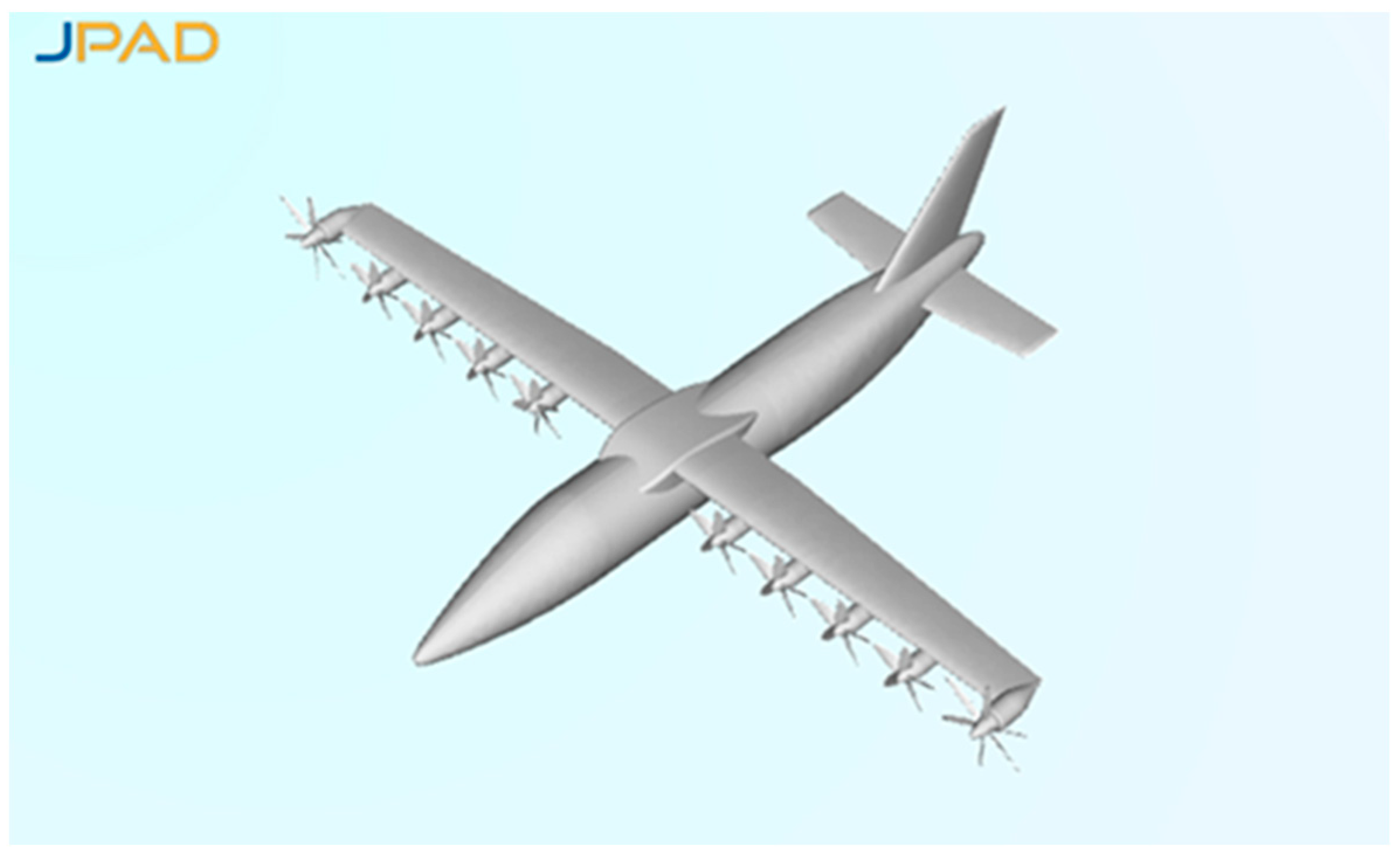
Figure 1.
A sketch of aircraft geometry, commuter aircraft 19 pax, obtained by means of JPAD.
Figure 1.
A sketch of aircraft geometry, commuter aircraft 19 pax, obtained by means of JPAD.
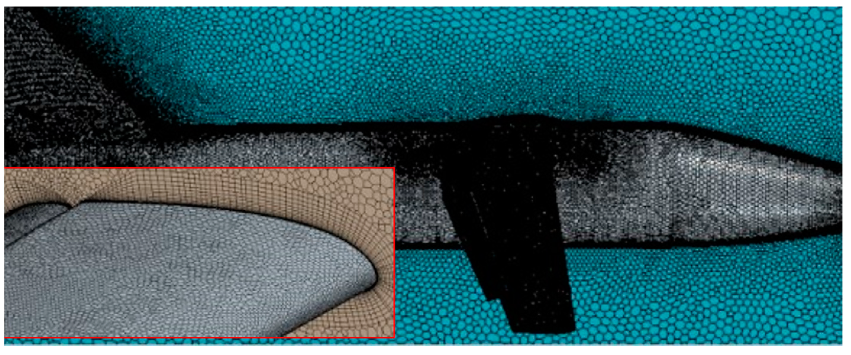
Figure 2.
Polyhedral mesh: symmetry plane near aircraft.
Figure 2.
Polyhedral mesh: symmetry plane near aircraft.
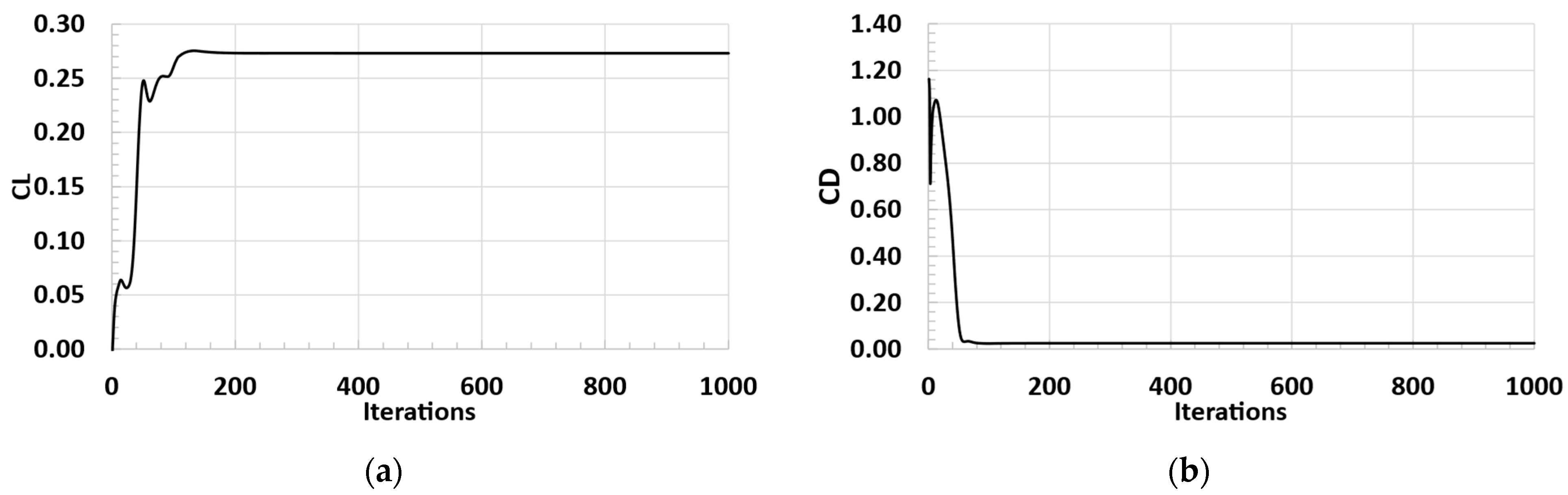
Figure 3.
Convergence plot for lift coefficient (a) and drag coefficient (b). Cruise condition, M = 0.32, Re = 9.2 Mil.
Figure 3.
Convergence plot for lift coefficient (a) and drag coefficient (b). Cruise condition, M = 0.32, Re = 9.2 Mil.
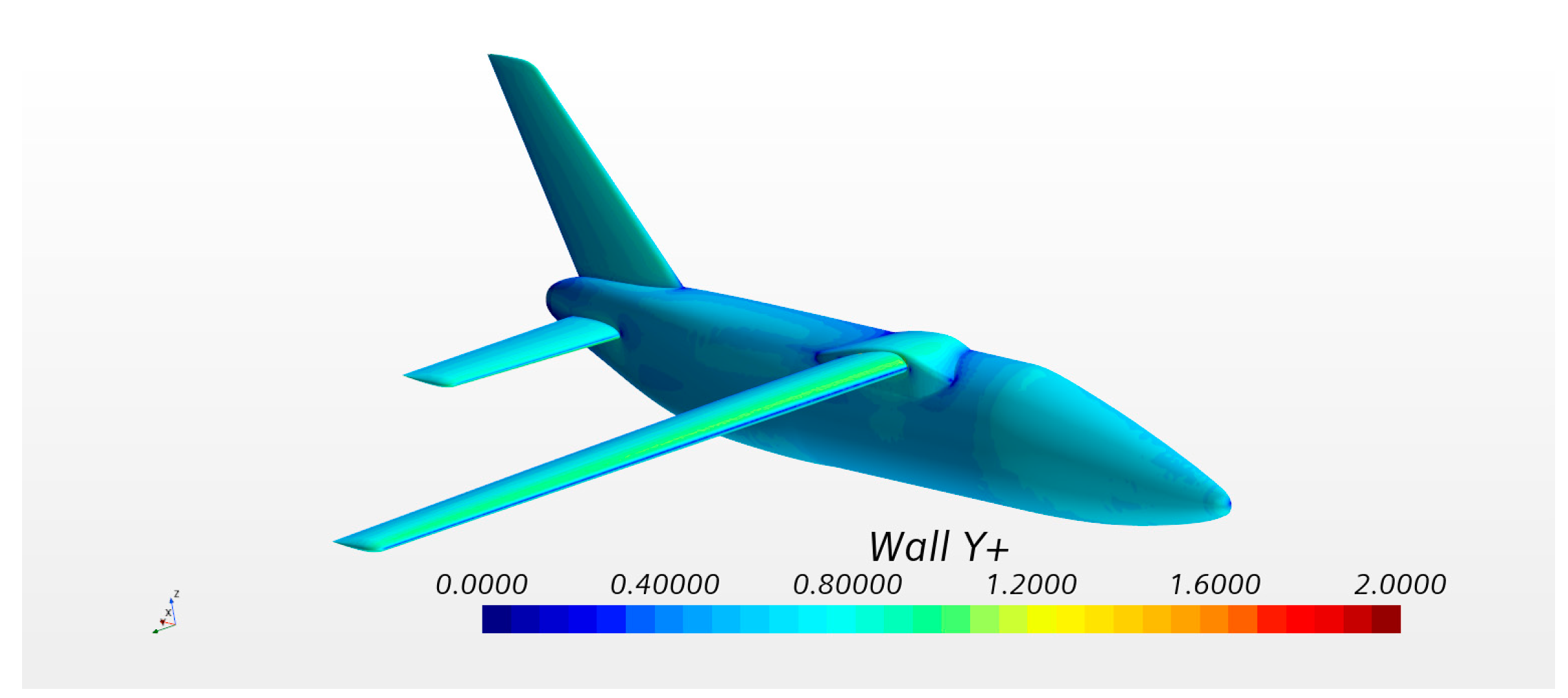
Figure 4.
Wall Y+ map, Star-CCM+, cruise condition, M = 0.32, Re = 9.2 Mil.
Figure 4.
Wall Y+ map, Star-CCM+, cruise condition, M = 0.32, Re = 9.2 Mil.
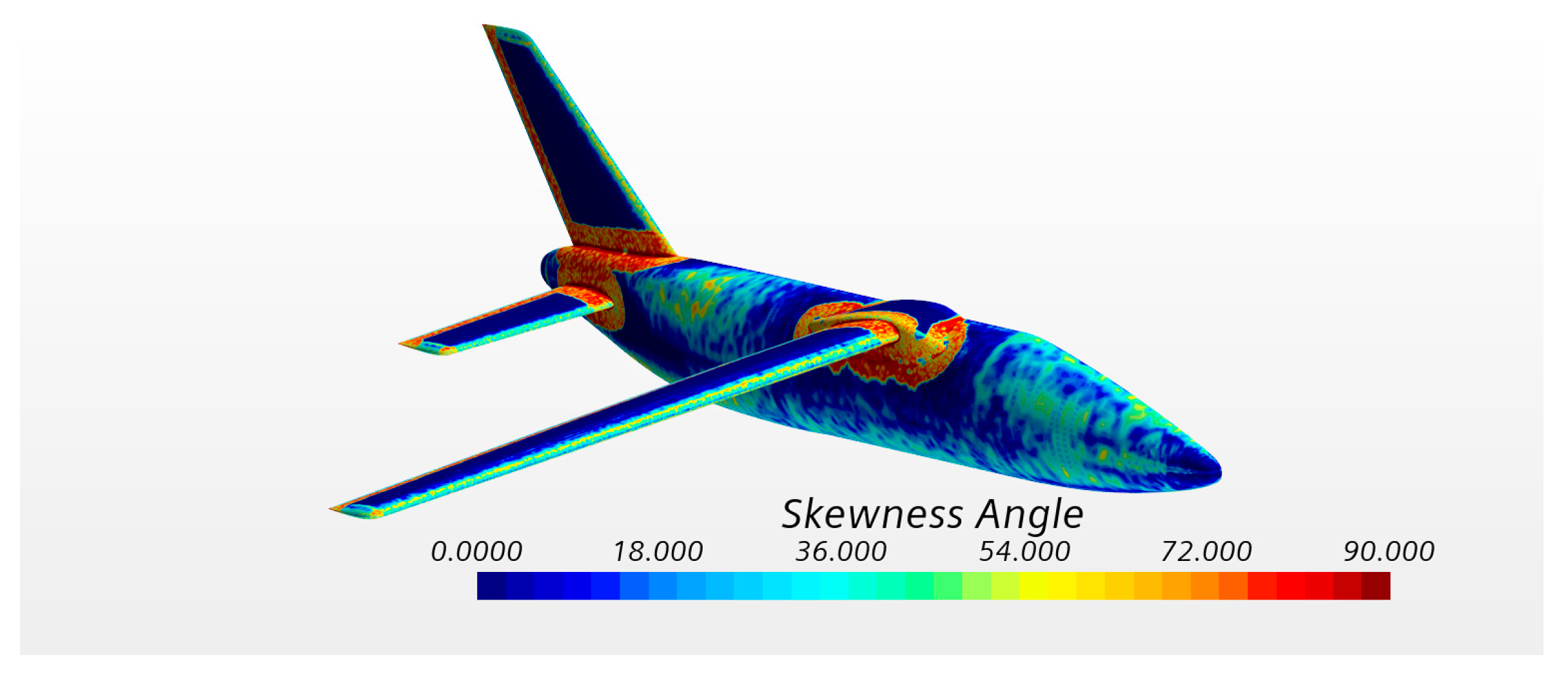
Figure 5.
Skewness angle map, Star-CCM+, cruise condition, M = 0.32, Re = 9.2 Mil.
Figure 5.
Skewness angle map, Star-CCM+, cruise condition, M = 0.32, Re = 9.2 Mil.
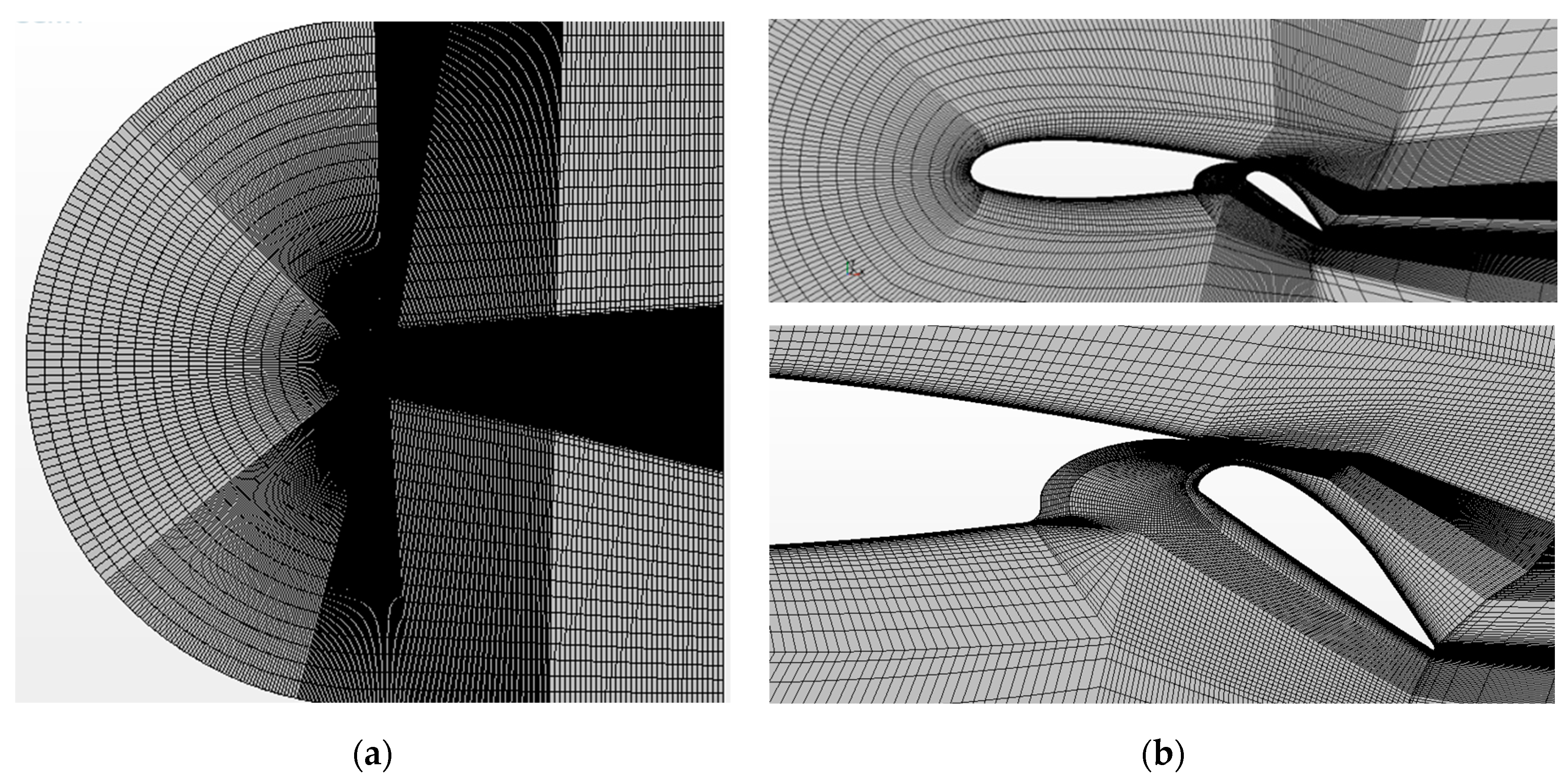
Figure 6.
Two-dimensional mesh for flapped airfoil analysis: (a) Global overview of C-shape domain; (b) mesh details around the airfoil and flap.
Figure 6.
Two-dimensional mesh for flapped airfoil analysis: (a) Global overview of C-shape domain; (b) mesh details around the airfoil and flap.
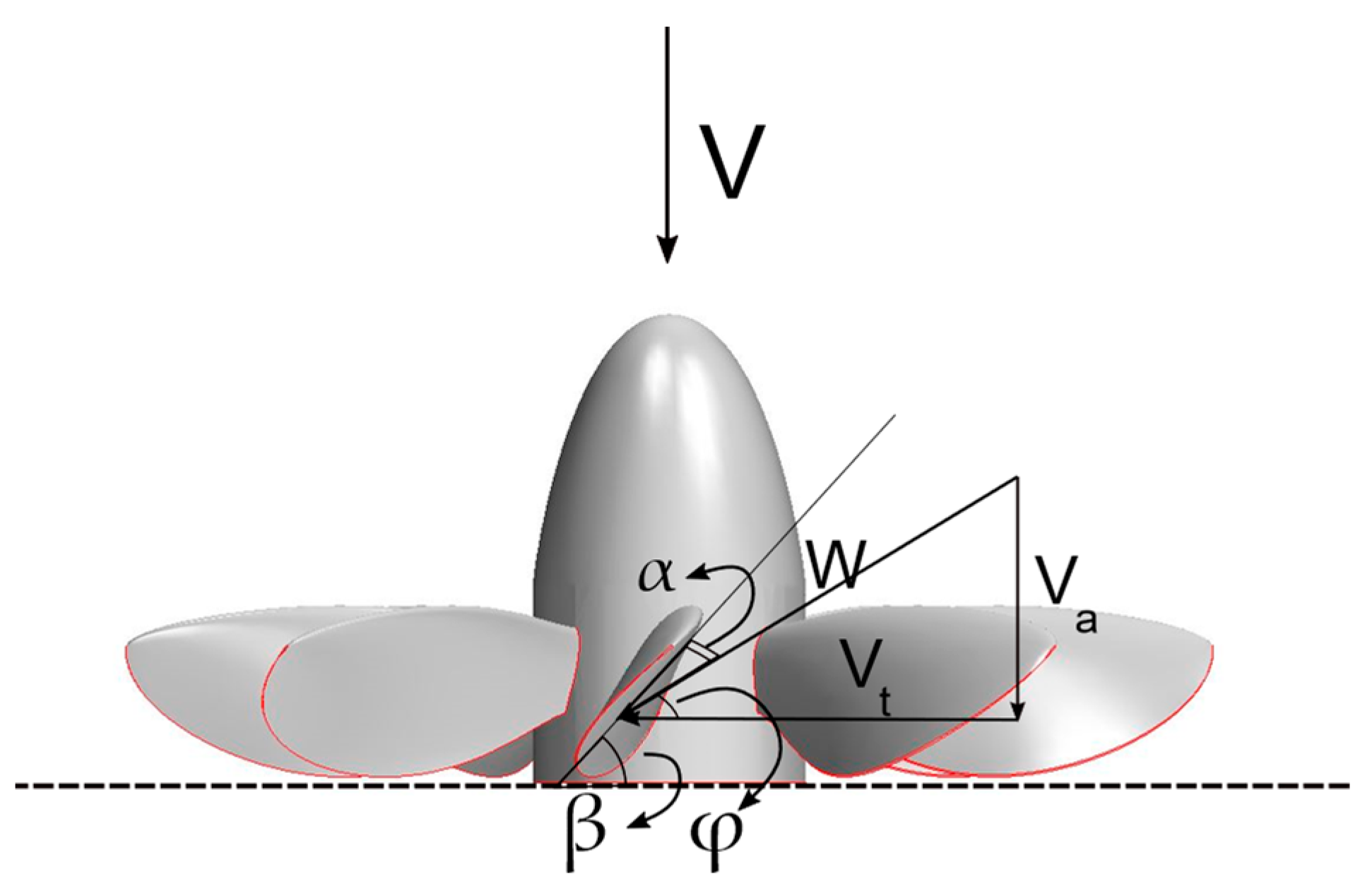
Figure 7.
Blade geometry definition and velocity of interest: α is AoA for the blade element, β is the geometric pitch angle, φ is the helix angle, Vt is the tangential velocity component, Va is the axial velocity component, and W is the resultant velocity.
Figure 7.
Blade geometry definition and velocity of interest: α is AoA for the blade element, β is the geometric pitch angle, φ is the helix angle, Vt is the tangential velocity component, Va is the axial velocity component, and W is the resultant velocity.
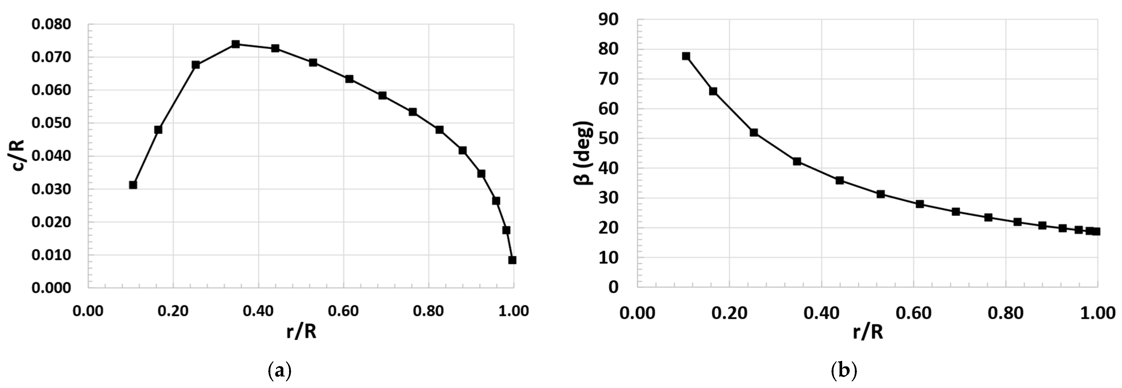
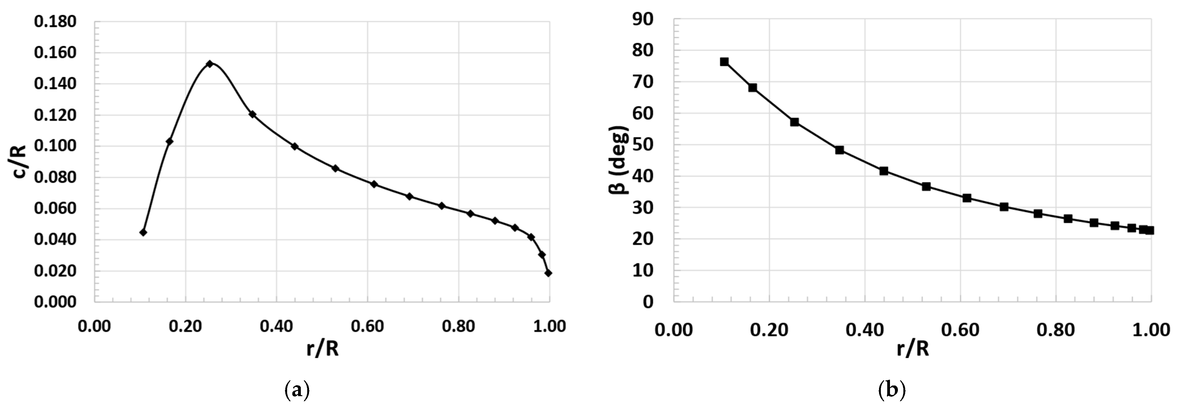
Figure 8.
TIP propeller designed with MIL approach. (a) Chord distribution. (b) Pitch angle distribution.
Figure 8.
TIP propeller designed with MIL approach. (a) Chord distribution. (b) Pitch angle distribution.
Figure 9.
DEP propeller designed with Patterson’s approach. (a) Chord distribution. (b) Pitch angle distribution.
Figure 9.
DEP propeller designed with Patterson’s approach. (a) Chord distribution. (b) Pitch angle distribution.
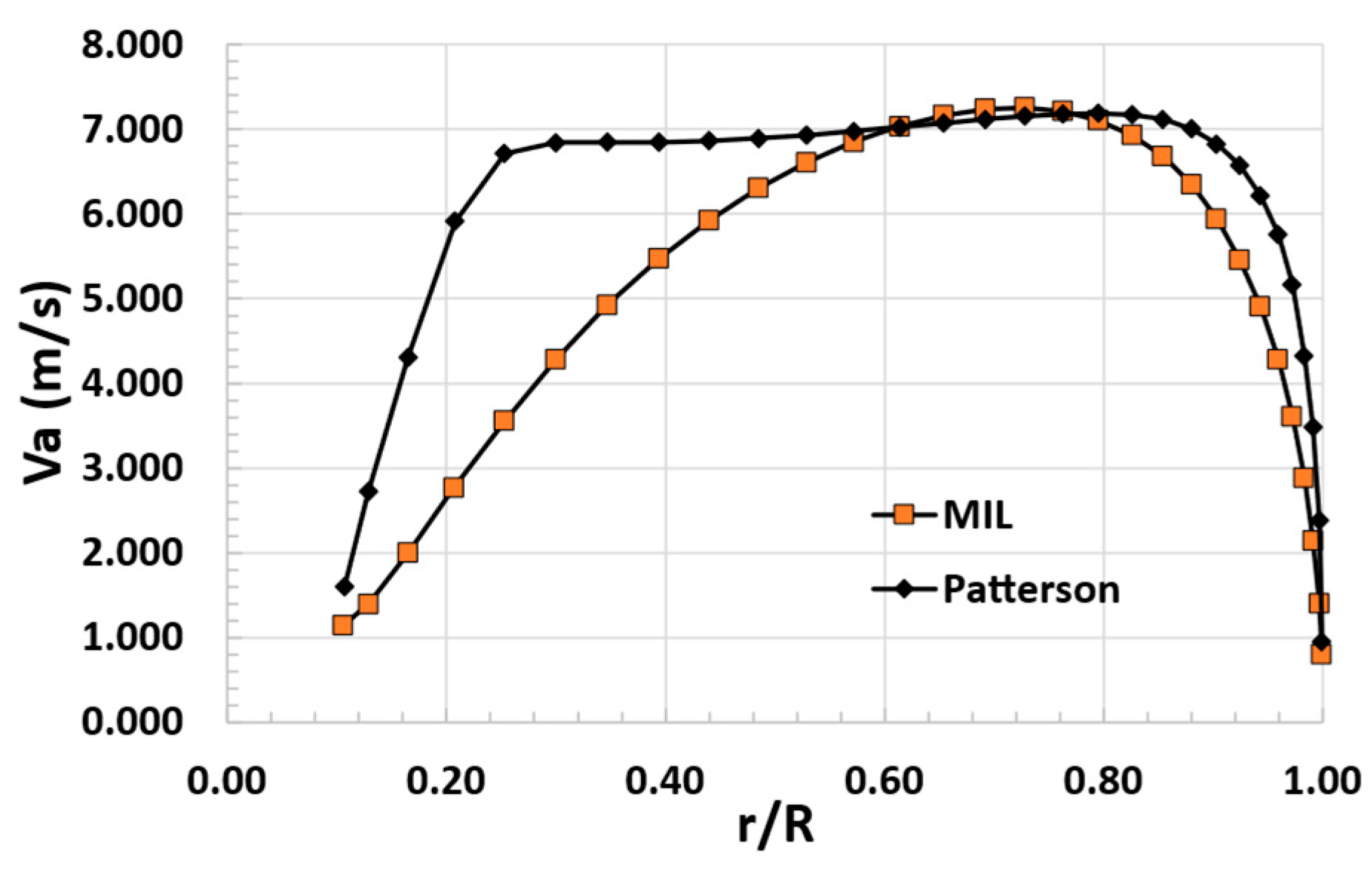
Figure 10.
Induced axial speed Va (m/s) for DEP propeller designed following Patterson approach and the equivalent one designed following the MIL approach.
Figure 10.
Induced axial speed Va (m/s) for DEP propeller designed following Patterson approach and the equivalent one designed following the MIL approach.
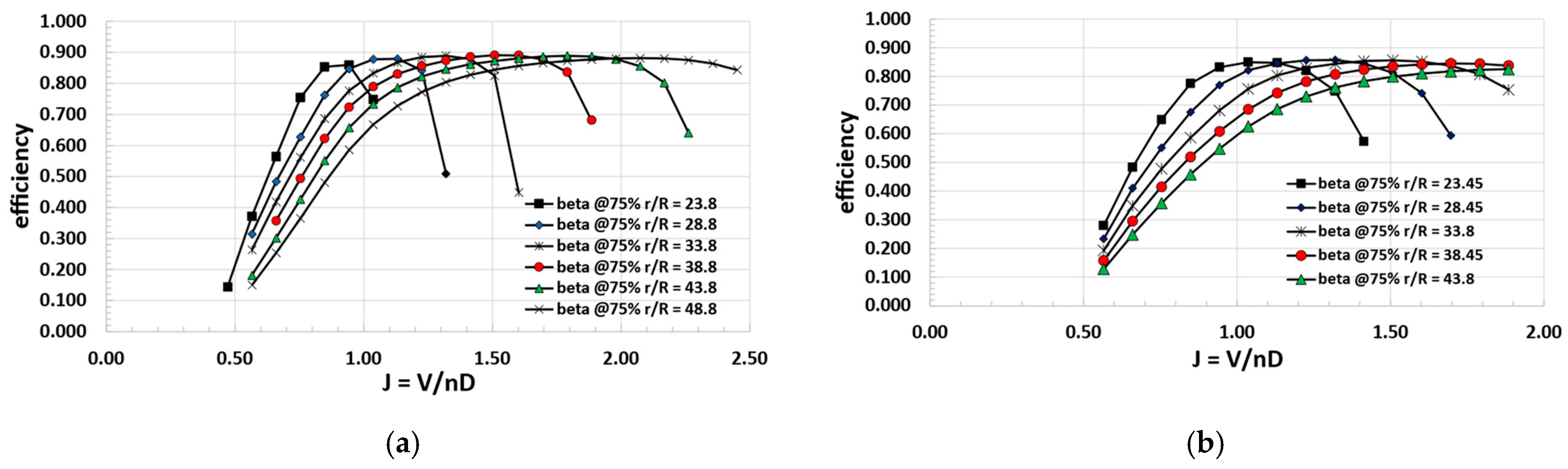
Figure 11.
Propellers efficiency map (different blade pitch angles). (a) Tip propeller. (b) DEP propeller.
Figure 11.
Propellers efficiency map (different blade pitch angles). (a) Tip propeller. (b) DEP propeller.
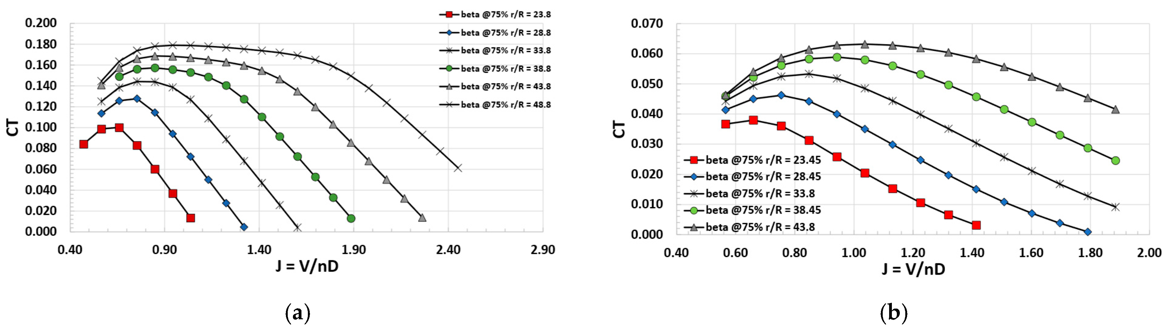
Figure 12.
Propellers thrust coefficient map (different blade pitch angles). (a) Tip propeller. (b) DEP propeller.
Figure 12.
Propellers thrust coefficient map (different blade pitch angles). (a) Tip propeller. (b) DEP propeller.
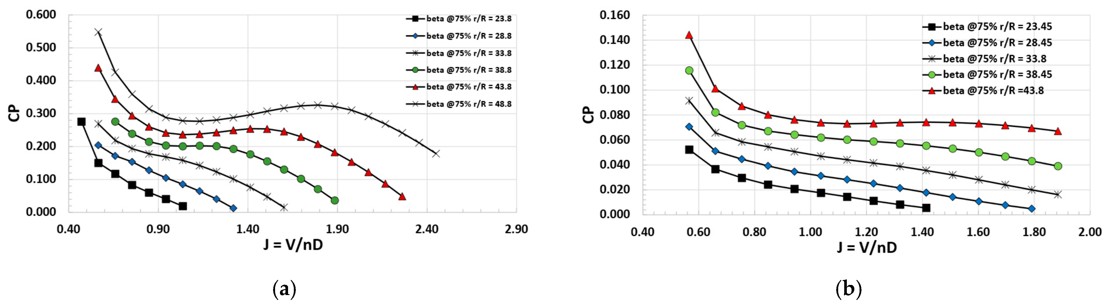
Figure 13.
Propeller power coefficient map (different blade pitch angles). (a) Tip propeller. (b) DEP propeller.
Figure 13.
Propeller power coefficient map (different blade pitch angles). (a) Tip propeller. (b) DEP propeller.
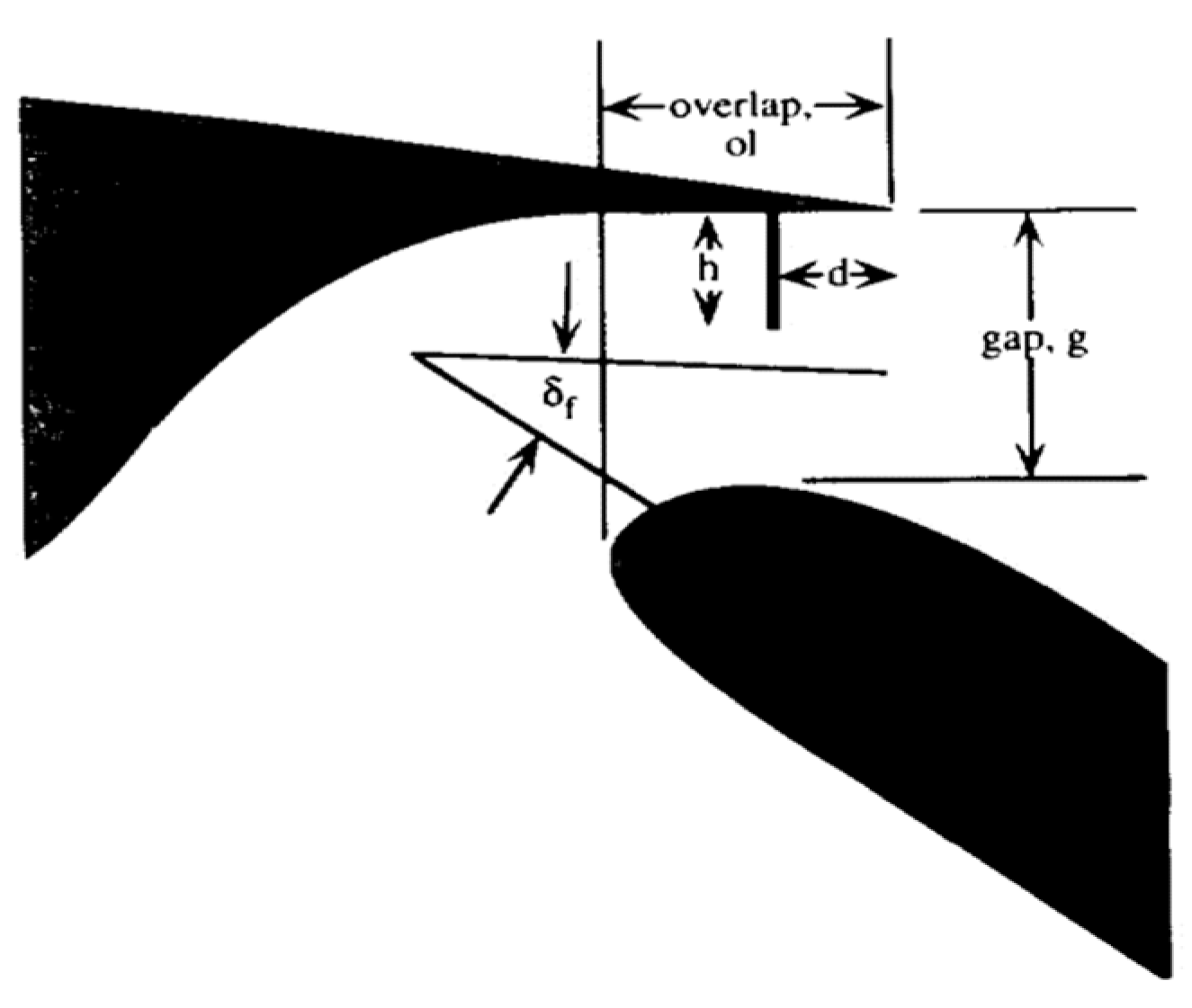
Figure 14.
Flap positioning main parameters: gap and overlap definition.
Figure 14.
Flap positioning main parameters: gap and overlap definition.
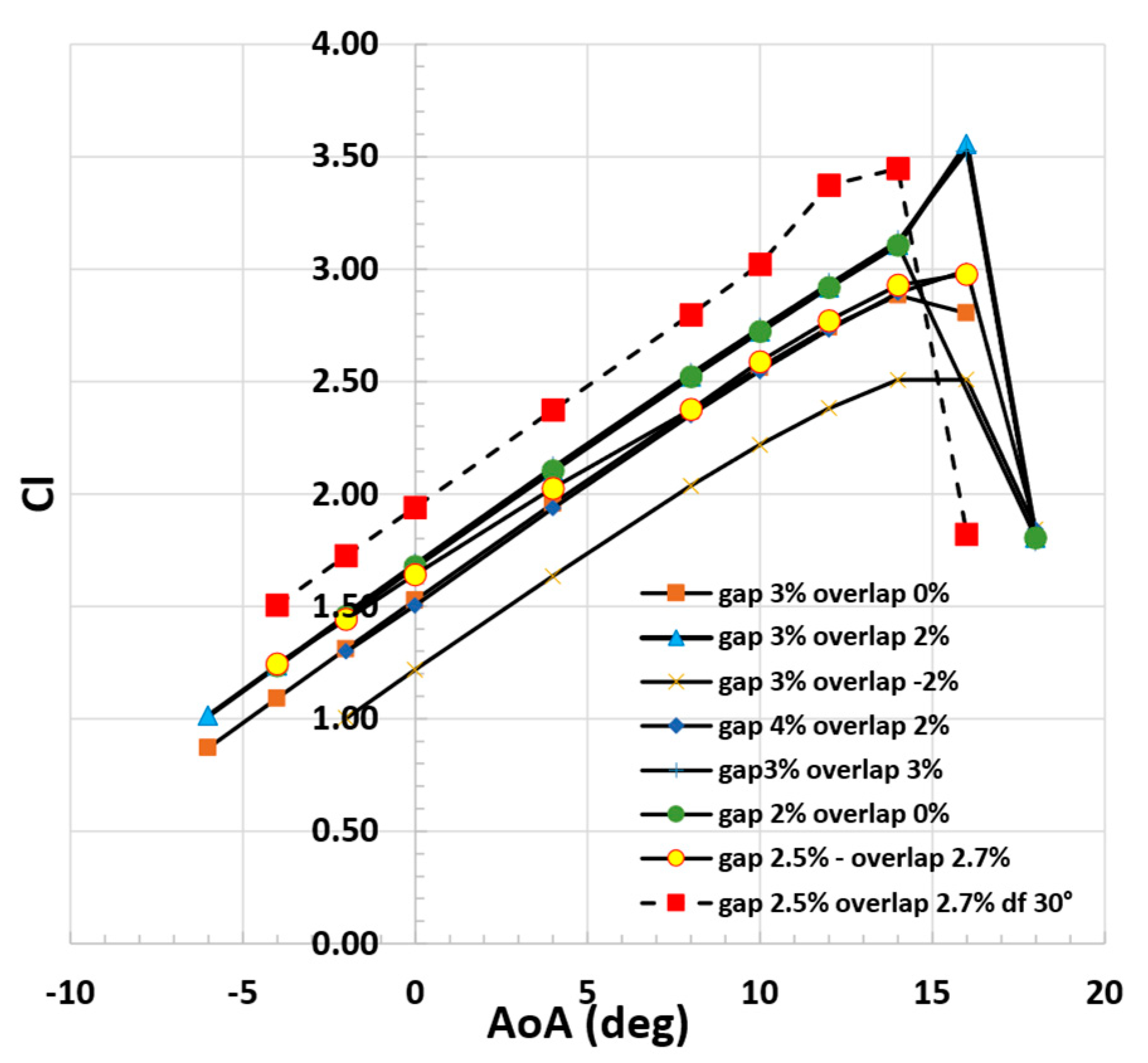
Figure 15.
Numerical results in terms of lift coefficient curves of 2D analysis at different flap positions, landing condition, M = 0.15, Re = 5.7 × 10⁶.
Figure 15.
Numerical results in terms of lift coefficient curves of 2D analysis at different flap positions, landing condition, M = 0.15, Re = 5.7 × 10⁶.
Figure 16.
Wing–fuselage fairing geometries without (a) and with (b) fillet.
Figure 16.
Wing–fuselage fairing geometries without (a) and with (b) fillet.
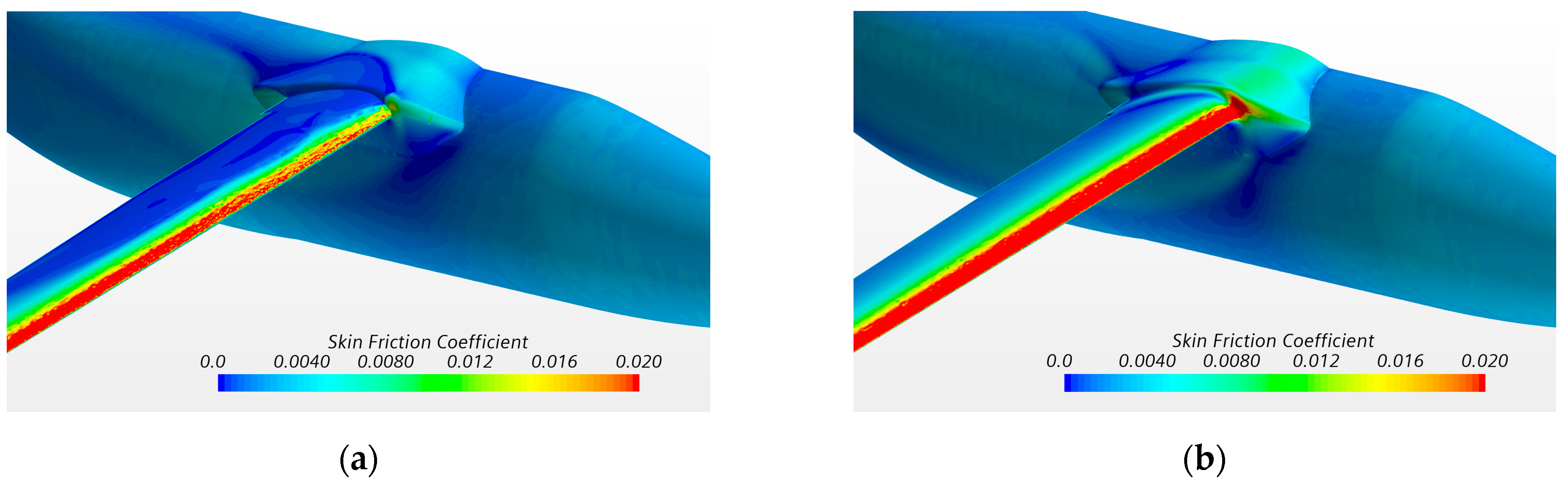
Figure 17.
Effect of the wing–fuselage fillet on the flow separation (skin friction map), AoA equal to 14 deg. (a) Geometry without fillet. (b) Geometry with fillet.
Figure 17.
Effect of the wing–fuselage fillet on the flow separation (skin friction map), AoA equal to 14 deg. (a) Geometry without fillet. (b) Geometry with fillet.
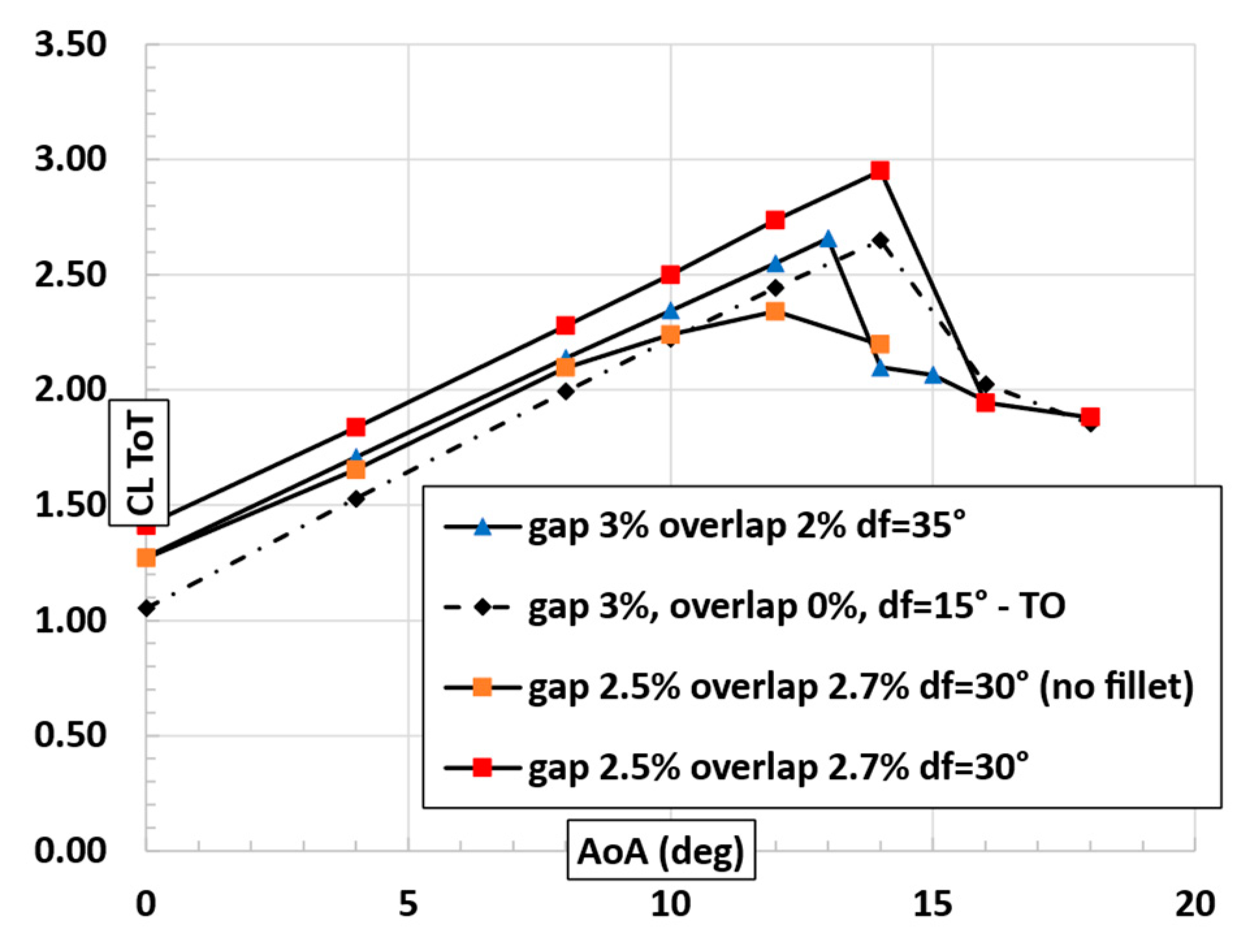
Figure 18.
Numerical results of 3D simulations in terms of global lift coefficient for different flap positions, landing condition, M = 0.15, Re = 5.7 × 10⁶.
Figure 18.
Numerical results of 3D simulations in terms of global lift coefficient for different flap positions, landing condition, M = 0.15, Re = 5.7 × 10⁶.
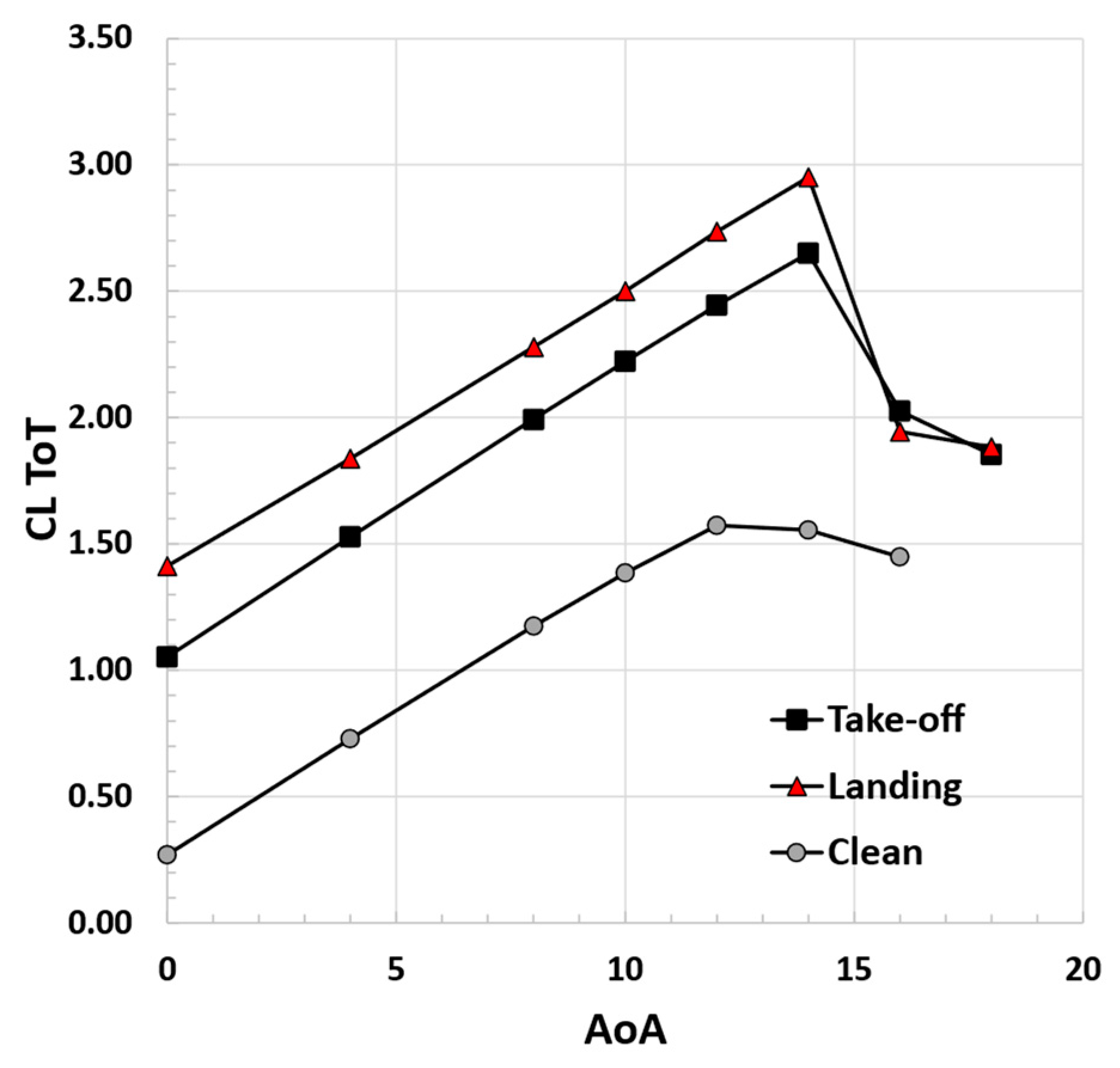
Figure 19.
Total lift coefficient curves for clean and flapped (take-off and landing setup) wing configurations, low-speed conditions, M = 0.15, Re = 5.7 × 10⁶.
Figure 19.
Total lift coefficient curves for clean and flapped (take-off and landing setup) wing configurations, low-speed conditions, M = 0.15, Re = 5.7 × 10⁶.
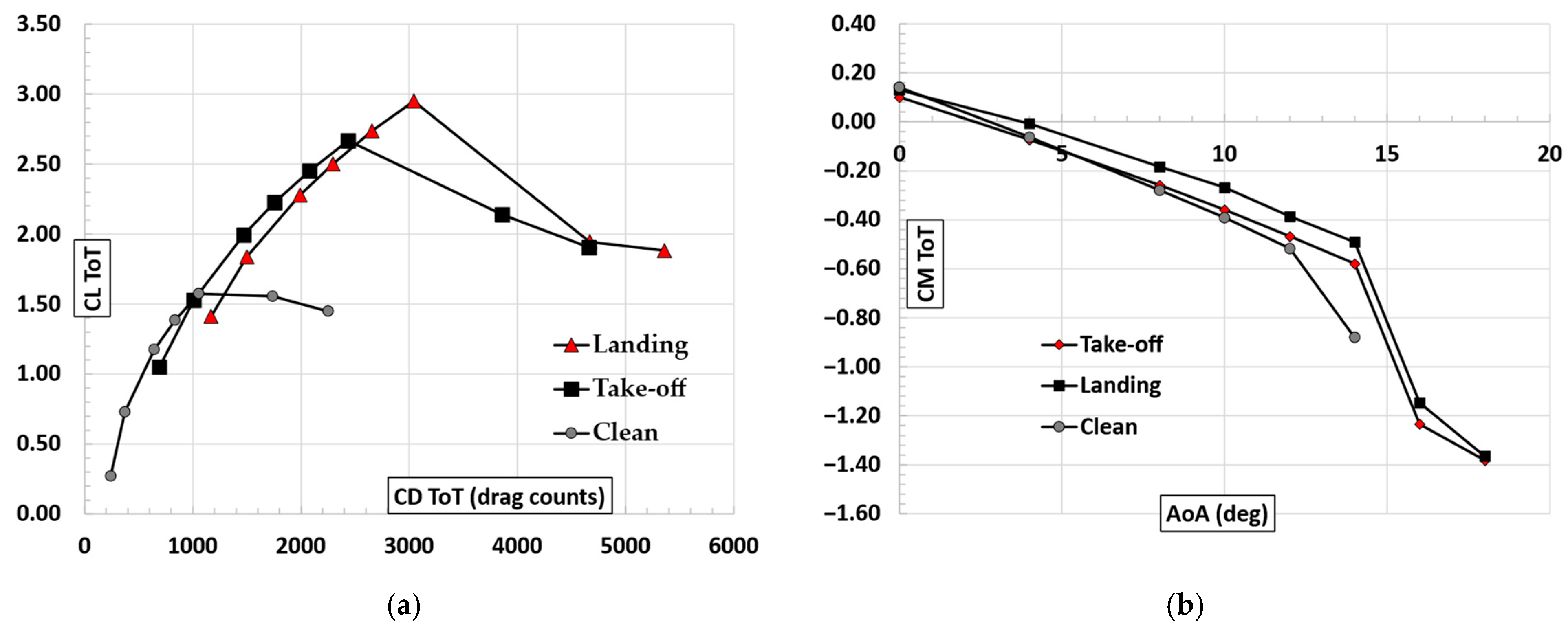
Figure 20.
Drag and pitching moment curves, take-off and landing condition, M = 0.15, Re = 5.7 × 10⁶. (a) Drag polar (drag expressed in counts). (b) Pitching moment coefficient w.r.t. CG pos. (31% mac).
Figure 20.
Drag and pitching moment curves, take-off and landing condition, M = 0.15, Re = 5.7 × 10⁶. (a) Drag polar (drag expressed in counts). (b) Pitching moment coefficient w.r.t. CG pos. (31% mac).
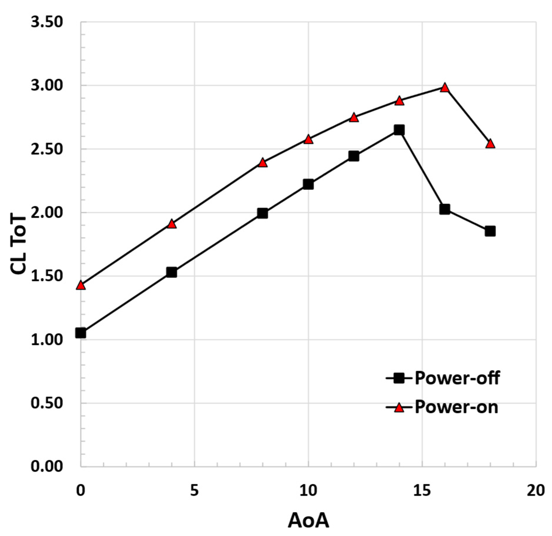
Figure 21.
Total lift coefficient curves for power-off and power-on take-off conditions, M = 0.15, Re = 5.7 × 10⁶, JTIP = 0.78, rpmTIP = 1600, JDEP = 0.89, rpmDEP = 2000.
Figure 21.
Total lift coefficient curves for power-off and power-on take-off conditions, M = 0.15, Re = 5.7 × 10⁶, JTIP = 0.78, rpmTIP = 1600, JDEP = 0.89, rpmDEP = 2000.
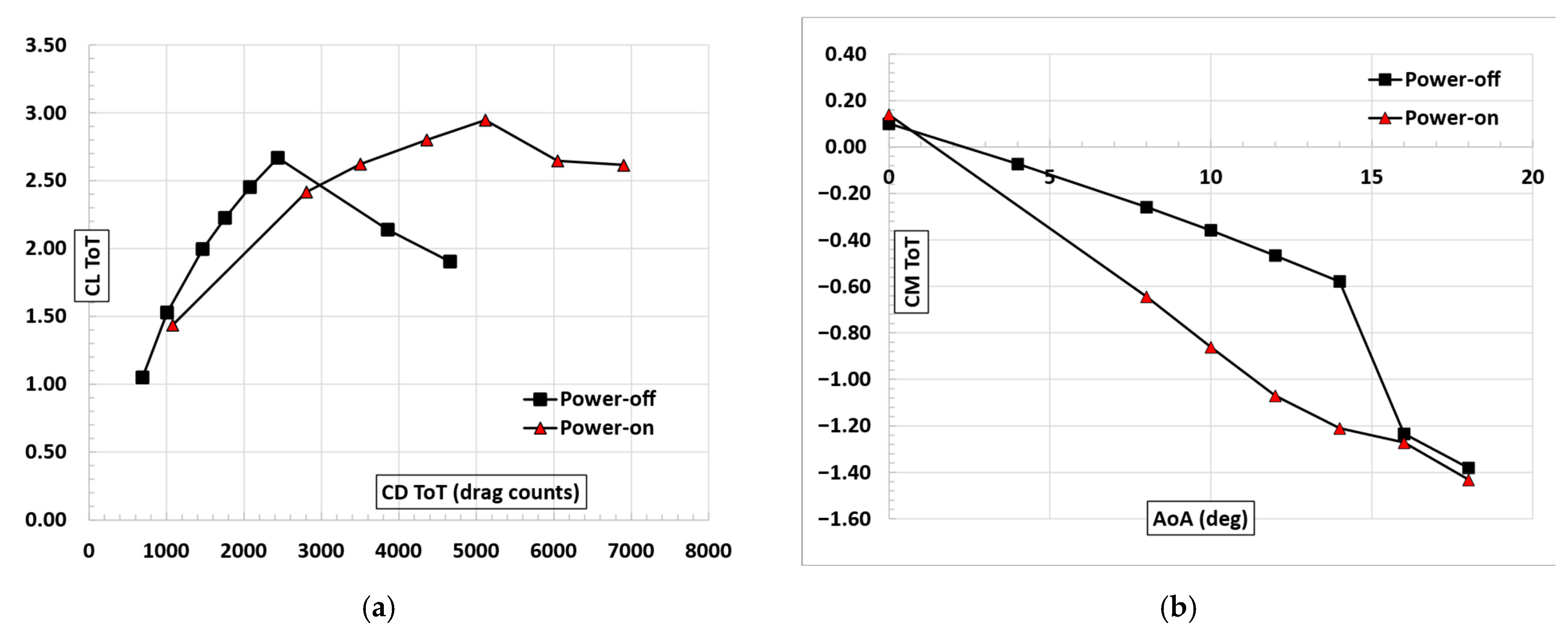
Figure 22.
Drag and pitching moment curves for power-off and power-on take-off conditions, M = 0.15, Re = 5.7 × 10⁶, JTIP = 0.78, rpmTIP = 1600, JDEP = 0.89, rpmDEP = 2000. (a) Drag polar (drag expressed in counts). (b) Pitching moment coefficient w.r.t. CG pos. (31% mac).
Figure 22.
Drag and pitching moment curves for power-off and power-on take-off conditions, M = 0.15, Re = 5.7 × 10⁶, JTIP = 0.78, rpmTIP = 1600, JDEP = 0.89, rpmDEP = 2000. (a) Drag polar (drag expressed in counts). (b) Pitching moment coefficient w.r.t. CG pos. (31% mac).
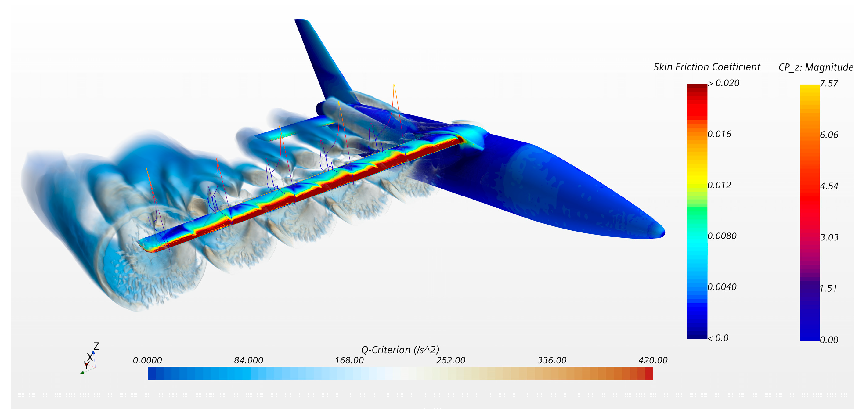
Figure 23.
Vorticity scene with the body skin friction contour and plot of pressure coefficient for sections located behind the propeller, AoA = 10 deg, take-off power-on, M = 0.15, Re = 5.7 × 10⁶, JTIP = 0.78, rpmTIP = 1600, JDEP = 0.89, rpmDEP = 2000.
Figure 23.
Vorticity scene with the body skin friction contour and plot of pressure coefficient for sections located behind the propeller, AoA = 10 deg, take-off power-on, M = 0.15, Re = 5.7 × 10⁶, JTIP = 0.78, rpmTIP = 1600, JDEP = 0.89, rpmDEP = 2000.
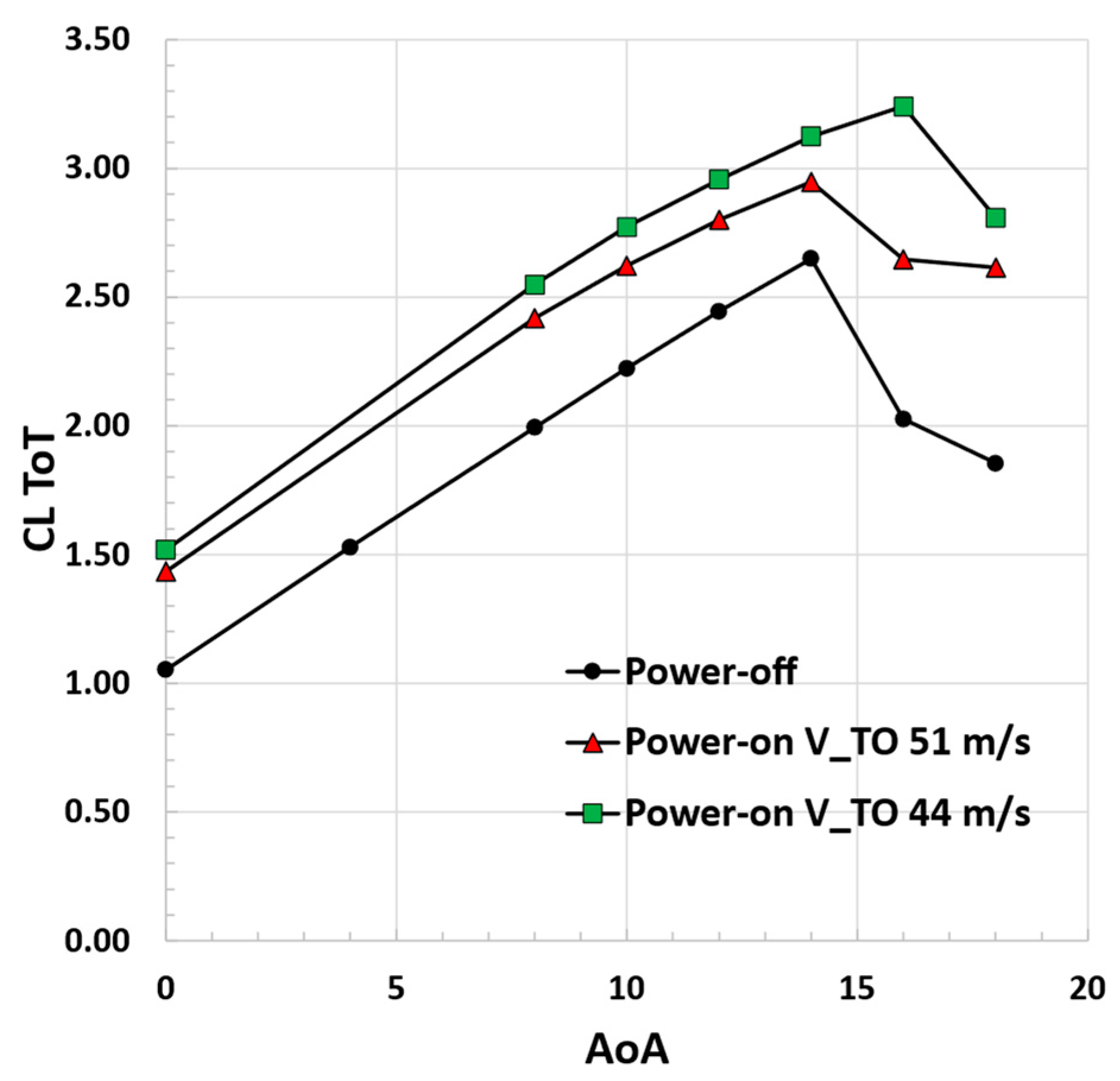
Figure 24.
Total lift coefficient curves for power-off and power-on take-off conditions, VTO = 44 m/s and VTO = 51 m/s, Re = 5.7 × 10⁶, JTIP = 0.78, rpmTIP = 1600, JDEP = 0.89, rpmDEP = 2000.
Figure 24.
Total lift coefficient curves for power-off and power-on take-off conditions, VTO = 44 m/s and VTO = 51 m/s, Re = 5.7 × 10⁶, JTIP = 0.78, rpmTIP = 1600, JDEP = 0.89, rpmDEP = 2000.
Figure 25.
Drag and pitching moment curves, take-off condition VTO = 44 m/s and VTO = 51 m/s, Re = 5.7 × 10⁶, JTIP = 0.78, rpmTIP = 1600, JDEP = 0.89, rpmDEP = 2000. (a) Drag polar (drag expressed in counts). (b) Pitching moment coefficient w.r.t. CG pos. (31% mac).
Figure 25.
Drag and pitching moment curves, take-off condition VTO = 44 m/s and VTO = 51 m/s, Re = 5.7 × 10⁶, JTIP = 0.78, rpmTIP = 1600, JDEP = 0.89, rpmDEP = 2000. (a) Drag polar (drag expressed in counts). (b) Pitching moment coefficient w.r.t. CG pos. (31% mac).
Table 1.
Relevant data of innovative aircraft configuration.
Table 1.
Relevant data of innovative aircraft configuration.
| Wing |
| Sw | 33.94 m2 |
| AR | 13 |
| root chord | 1.851 |
| Kink position | 2.88 m |
| TR | 0.65 |
| MAC | 1.645 m |
| LE sweep angle | 0 deg |
| TE sweep angle (kink-tip) | 4 deg |
| wing incidence | 3 deg |
| tip washout | −3 deg |
| Airfoil (root, kink, tip)
| NACA 23018/18/15 |
| Fuselage |
| Length | 18 m |
| Cabin Diameter | 2.150 m |
| Cabin Height | 2.262 m |
| Horizontal tail |
| Sh | 10.6 m2 |
| ARh | 4.6 |
| root chord | 1.76 |
| TR | 0.72 |
| LE sweep angle | 8 deg |
| Airfoil | NACA 0012 |
| Vertical tail |
| Sv | 10.6 m2 |
| ARv | 1.6 |
| root chord | 3.345 m |
| TR | 0.37 |
| LE sweep angle | 45 deg |
| Airfoil | NACA 0012 |
| Weight and Balance |
| MTOM | 8139 kg |
| CG (%mac) | [30–40%, 0.0, −25%]
Wing reference frame |
Table 2.
Mesh and numerical model parameters.
Table 2.
Mesh and numerical model parameters.
| Mesh Type | Unstructured (Polyhedral Cells) |
|---|
| Number of cells | ~8,500,000 |
| Number of prism layer | 33 |
| Wall distance of the first cell | 6 × 10⁻⁶ m |
| Turbulence models | Spalart–Allmaras (SA) |
| Flow model | Ideal gas |
| Solver | Steady Coupled implicit |
| Number of iterations per AoA | 1000 |
| Boundary conditions | Inflow: Free Stream |
| Outflow: Pressure Outlet |
Table 3.
Flight conditions.
Table 3.
Flight conditions.
| | Low Speed | Climb | Cruise |
|---|
| Mach number | 0.15 | 0.26 | 0.317 |
| Reynolds number | 5.7 × 10⁶ | 8.7 × 10⁶ | 9.2 × 10⁶ |
| Reference altitude | S/L | 1500 m | 3048 m |
| Reference density | 1.225 kg/m3 | 1.058 kg/m3 | 0.909 kg/m3 |
| Speed of sound | 340.3 m/s | 334.5 m/s | 328.4 m/s |
Table 4.
Relevant data for 2D analysis.
Table 4.
Relevant data for 2D analysis.
| Low-Speed Conditions |
|---|
| Mesh type | 2D-Structured |
| Number of cells | 86,179 |
| Mach number | 0.15 |
| Reynolds number | 5.7 × 10⁶ |
| Speed of sound | 340.3 m/s |
| Number of iterations per AoA | ~1000 |
Table 5.
Power requirements for each flight phase.
Table 5.
Power requirements for each flight phase.
| | Altitude | Speed | Shaft Power TIP | Shaft Power DEP |
|---|
| Take-Off | 0 m | 51 m/s | 217 kW | 126 kW |
| Climb | 1500 m | 94 m/s | 225 kW | 131 kW |
| Cruise | 3000 m | 104 m/s | 221 kW | 129 kW |
| Descent | 1500 m | 66 m/s | 32 kW | 49 kW |
| Landing | 0 m | 54 m/s | 16 kW | 6 kW |
Table 6.
DEP and TIP propeller geometries (r, blade station, R, blade radius, c, blade local chord).
Table 6.
DEP and TIP propeller geometries (r, blade station, R, blade radius, c, blade local chord).
| DEP Propeller | TIP Propeller |
|---|
| r/R | c/R | Blade Pitch Angle β (deg) | r/R | c/R | Blade Pitch Angle β (deg) |
|---|
| 0.101 | 0.04 | 80.70 | 0.106 | 0.031 | 82.63 |
| 0.103 | 0.042 | 80.36 | 0.129 | 0.037 | 77.97 |
| 0.111 | 0.049 | 79.35 | 0.165 | 0.048 | 70.79 |
| 0.124 | 0.061 | 77.73 | 0.207 | 0.059 | 63.49 |
| 0.142 | 0.079 | 75.59 | 0.253 | 0.068 | 56.96 |
| 0.165 | 0.105 | 73.04 | 0.3 | 0.072 | 51.36 |
| 0.192 | 0.12 | 69.1 | 0.347 | 0.074 | 47.25 |
| 0.224 | 0.129 | 64.58 | 0.394 | 0.074 | 43.78 |
| 0.259 | 0.126 | 59.52 | 0.44 | 0.073 | 40.85 |
| 0.298 | 0.113 | 54.38 | 0.485 | 0.071 | 38.37 |
| 0.34 | 0.103 | 49.81 | 0.529 | 0.068 | 36.26 |
| 0.384 | 0.094 | 45.76 | 0.572 | 0.066 | 34.44 |
| 0.43 | 0.086 | 42.21 | 0.614 | 0.063 | 32.87 |
| 0.478 | 0.079 | 39.1 | 0.654 | 0.061 | 31.51 |
| 0.526 | 0.073 | 36.4 | 0.692 | 0.058 | 30.33 |
| 0.575 | 0.068 | 34.07 | 0.728 | 0.056 | 29.28 |
| 0.623 | 0.063 | 32.06 | 0.763 | 0.053 | 28.37 |
| 0.671 | 0.059 | 30.34 | 0.795 | 0.051 | 27.56 |
| 0.717 | 0.056 | 28.86 | 0.826 | 0.048 | 26.85 |
| 0.761 | 0.053 | 27.61 | 0.854 | 0.045 | 26.23 |
| 0.803 | 0.05 | 26.56 | 0.88 | 0.042 | 25.68 |
| 0.841 | 0.047 | 25.7 | 0.903 | 0.038 | 25.21 |
| 0.877 | 0.045 | 25 | 0.924 | 0.035 | 24.81 |
| 0.908 | 0.042 | 24.47 | 0.943 | 0.031 | 24.47 |
| 0.936 | 0.039 | 24.1 | 0.959 | 0.026 | 24.2 |
| 0.958 | 0.035 | 23.89 | 0.972 | 0.022 | 23.99 |
| 0.976 | 0.03 | 23.83 | 0.983 | 0.018 | 23.83 |
| 0.989 | 0.023 | 23.9 | 0.991 | 0.013 | 23.73 |
| 0.997 | 0.013 | 24.02 | 0.997 | 0.008 | 23.68 |
| 0.999 | 0.006 | 24.09 | 0.999 | 0.005 | 23.65 |
Table 7.
Aerodynamic data of M114 and SDA1075 blade airfoil, XFOIL M = 0.15, Re = 3 × 10⁶.
Table 7.
Aerodynamic data of M114 and SDA1075 blade airfoil, XFOIL M = 0.15, Re = 3 × 10⁶.
| M114 Airfoil | SDA1075 Airfoil |
|---|
| AoA | cl | cd | AoA | cl | cd |
|---|
| −6 | 0.257 | 0.00818 | −6 | −0.467 | 0.0073 |
| −5 | 0.382 | 0.00697 | −5 | −0.362 | 0.0068 |
| −4 | 0.51 | 0.00641 | −4 | −0.256 | 0.0064 |
| −3 | 0.636 | 0.00628 | −3 | −0.151 | 0.0059 |
| −2 | 0.762 | 0.00604 | −2 | −0.045 | 0.0056 |
| −1 | 0.88 | 0.00617 | −1 | 0.061 | 0.0053 |
| 0 | 1.001 | 0.0063 | 0 | 0.167 | 0.0051 |
| 1 | 1.12 | 0.00656 | 1 | 0.273 | 0.005 |
| 2 | 1.239 | 0.00668 | 2 | 0.378 | 0.005 |
| 3 | 1.358 | 0.00699 | 3 | 0.478 | 0.0048 |
| 4 | 1.475 | 0.00732 | 4 | 0.591 | 0.0048 |
| 5 | 1.59 | 0.00779 | 5 | 0.714 | 0.0054 |
| 6 | 1.704 | 0.00825 | 6 | 0.842 | 0.0061 |
| 7 | 1.815 | 0.00867 | 7 | 0.959 | 0.0071 |
| 8 | 1.921 | 0.00959 | 8 | 1.082 | 0.0085 |
| 9 | 2.019 | 0.01055 | 9 | 1.21 | 0.01 |
| 10 | 2.083 | 0.0118 | 10 | 1.317 | 0.0113 |
| 11 | 2.101 | 0.0232 | 11 | 1.389 | 0.0127 |
| 12 | 2.084 | 0.02084 | 12 | 1.458 | 0.0141 |
| 13 | 2.03 | 0.02262 | 13 | 1.494 | 0.0158 |
| 14 | 1.951 | 0.03242 | 14 | 1.535 | 0.0179 |
| 15 | 1.844 | 0.03692 | 15 | 1.57 | 0.0211 |
| 16 | 1.711 | 0.04214 | 16 | 1.597 | 0.0261 |
| 17 | 1.562 | 0.04865 | 17 | 1.605 | 0.0341 |
| 18 | 1.408 | 0.05684 | 18 | 1.598 | 0.0452 |
| 19 | 1.257 | 0.06743 | 19 | 1.569 | 0.0605 |
| 20 | 1.112 | 0.08102 | 20 | 1.509 | 0.0816 |
Table 8.
Propellers take-off operating points. Both DEP and TIP propellers have a right-handed rotation.
Table 8.
Propellers take-off operating points. Both DEP and TIP propellers have a right-handed rotation.
| | D (m) | J | CT | n (rpm) | Pitch Angle @.75 r/R (deg) | Efficiency | Power (kW) |
|---|
| DEP | 1.89 | 0.89 | 0.138 | 2000 | 28.4 | 0.82 | 126 |
| TIP | 2.54 | 0.78 | 0.1015 | 1600 | 23.8 | 0.86 | 217 |
Table 9.
Main flap characteristics.
Table 9.
Main flap characteristics.
| Type | Fowler |
| Flap/Wing chord ratio | 0.3 |
| Inner station | 12% wingspan |
| Outer station | 80% wingspan |
| Airfoil (root, kink, tip) | NACA 23018/18/15 |
Table 10.
Numerical results of 2D analysis at different flap positions, landing condition, M = 0.15, Re = 5.7 × 10⁶.
Table 10.
Numerical results of 2D analysis at different flap positions, landing condition, M = 0.15, Re = 5.7 × 10⁶.
| Gap | Overlap | Deflection | Cl max | Cl α | Cl0 |
|---|
| 3% | 0% | 35 deg | 2.88 | 0.108 | 1.53 |
| 3% | −2% | 35 deg | 2.51 | 0.105 | 1.22 |
| 3% | 2% | 35 deg | 3.56 | 0.107 | 1.68 |
| 3% | 3% | 35 deg | 3.52 | 0.108 | 1.69 |
| 2% | 0% | 35 deg | 3.11 | 0.108 | 1.46 |
| 4% | 2% | 35 deg | 2.99 | 0.106 | 1.50 |
| 2.5% | 2.7% | 35 deg | 2.98 | 0.097 | 1.64 |
| 2.5% | 2.7% | 30 deg | 3.45 | 0.108 | 1.94 |
Table 11.
Flap position take-off.
Table 11.
Flap position take-off.
| Take-Off |
|---|
| Gap | 3% chord |
| Overlap | 0% chord |
| Deflection | 15 deg |
Table 12.
Flap position landing.
Table 12.
Flap position landing.
| Landing |
|---|
| Gap | 2.5% chord |
| Overlap | 2.7% chord |
| Deflection | 30 deg |
Table 13.
Numerical results for low-speed conditions, untrimmed maximum lift coefficient, moment coefficient calculated w.r.t. CG pos. (31% mac), M = 0.15, Re = 5.7 × 10⁶.
Table 13.
Numerical results for low-speed conditions, untrimmed maximum lift coefficient, moment coefficient calculated w.r.t. CG pos. (31% mac), M = 0.15, Re = 5.7 × 10⁶.
| | CLmax | CLα | CL0 | CMα | CM0 |
|---|
| Clean | 1.57 | 0.110 | 0.27 | −0.053 | 0.118 |
| Take Off | 2.65 | 0.118 | 1.05 | −0.045 | 0.100 |
| Landing | 2.95 | 0.108 | 1.41 | −0.039 | 0.130 |
Table 14.
Numerical results for low-speed conditions, trimmed maximum lift coefficient, moment coefficient calculated w.r.t. CG pos. (31% mac), M = 0.15, Re = 5.7 × 10⁶.
Table 14.
Numerical results for low-speed conditions, trimmed maximum lift coefficient, moment coefficient calculated w.r.t. CG pos. (31% mac), M = 0.15, Re = 5.7 × 10⁶.
| | CLmax | CM cg
(@AoA = 14 Deg) | VH | ΔCLH | CLmax trimmed |
|---|
| Take-Off | 2.65 | −0.593 | 1.5 | −0.12 | 2.53 |
| Landing | 2.95 | −0.491 | 1.5 | −0.10 | 2.85 |
Table 15.
Numerical results for take-off power-on condition, untrimmed maximum lift coefficient, moment coefficient calculated w.r.t. CG pos. (31% mac), M = 0.15, Re = 5.7 × 10⁶, JTIP = 0.78, rpmTIP = 1600, JDEP = 0.89, rpmDEP = 2000.
Table 15.
Numerical results for take-off power-on condition, untrimmed maximum lift coefficient, moment coefficient calculated w.r.t. CG pos. (31% mac), M = 0.15, Re = 5.7 × 10⁶, JTIP = 0.78, rpmTIP = 1600, JDEP = 0.89, rpmDEP = 2000.
| Take Off | CLmax | CLα | CL0 | CMα | CM0 |
|---|
| power-off | 2.65 | 0.118 | 1.05 | −0.045 | 0.100 |
| power-on | 2.95 | 0.123 | 1.43 | −0.098 | 0.139 |
Table 16.
Numerical results for take-off, trimmed maximum lift coefficient, moment coefficient calculated w.r.t. CG pos. (31% mac), power-on conditions: JTIP = 0.78, rpmTIP = 1600, JDEP = 0.89, rpmDEP = 2000. M = 0.15, Re = 5.7 × 10⁶.
Table 16.
Numerical results for take-off, trimmed maximum lift coefficient, moment coefficient calculated w.r.t. CG pos. (31% mac), power-on conditions: JTIP = 0.78, rpmTIP = 1600, JDEP = 0.89, rpmDEP = 2000. M = 0.15, Re = 5.7 × 10⁶.
| Take Off | CLmax | CM cg
(@AoA = 14 Deg) | VH | ΔCLH | CLmax trimmed |
|---|
| power off | 2.657 | −0.593 | 1.5 | −0.12 | 2.53 |
| power on | 2.95 | −1.210 | 1.5 | −0.25 | 2.70 |
Table 17.
Numerical results for take-off power-on condition, untrimmed maximum lift coefficient, moment coefficient calculated w.r.t. CG pos. (31% mac), VTO = 44 m/s and VTO = 51 m/s, Re = 5.7 × 10⁶, JTIP = 0.78, rpmTIP = 1600, JDEP = 0.89, rpmDEP = 2000.
Table 17.
Numerical results for take-off power-on condition, untrimmed maximum lift coefficient, moment coefficient calculated w.r.t. CG pos. (31% mac), VTO = 44 m/s and VTO = 51 m/s, Re = 5.7 × 10⁶, JTIP = 0.78, rpmTIP = 1600, JDEP = 0.89, rpmDEP = 2000.
| Take Off | CLmax | CLα | CL0 | CMα | CM0 |
|---|
| power-off | 2.65 | 0.118 | 1.05 | −0.045 | 0.100 |
| power-on | 2.95 | 0.123 | 1.43 | −0.098 | 0.139 |
| power-on(reduced VTO) | 3.24 | 0.129 | 1.52 | −0.098 | 0.138 |
Table 18.
Numerical results for take-off power-on condition, trimmed maximum lift coefficient, moment coefficient calculated w.r.t. CG pos. (31% mac), VTO = 44 m/s and VTO = 51 m/s, Re = 5.7 × 10⁶, JTIP = 0.78, rpmTIP = 1600, JDEP = 0.89, rpmDEP = 2000.
Table 18.
Numerical results for take-off power-on condition, trimmed maximum lift coefficient, moment coefficient calculated w.r.t. CG pos. (31% mac), VTO = 44 m/s and VTO = 51 m/s, Re = 5.7 × 10⁶, JTIP = 0.78, rpmTIP = 1600, JDEP = 0.89, rpmDEP = 2000.
| Take Off | CLmax | CM cg
(@AoA = 14 Deg) | VH | ΔCLH | CLmax trimmed |
|---|
| power off | 2.67 | −0.593 | 1.5 | −0.12 | 2.53 |
| power on | 2.95 | −1.210 | 1.5 | −0.25 | 2.70 |
| power-on(reduced VTO) | 3.24 | −1.268 | 1.5 | −0.26 | 2.98 |
Table 19.
DEP effect on the take-off distance.
Table 19.
DEP effect on the take-off distance.
| Take Off | CLmax trimmed | Take-Off Stall Speed
(m/s) | Take-Off Distance
(m) | Δ% |
|---|
| Reference | 2.0 | 40.37 | 507 | |
| Power-off | 2.53 | 38.96 | 435 | −14% |
| Power-on | 2.70 | 37.72 | 407 | −19% |
Power-on
(reduced VTO) | 2.98 | 35.90 | 365 | −27% |


