
An Efficient Task Synthesis Method Based on Subspace Differential Patterns for Arrangements of Event Intervals Mining in the Avionics Cloud System Architecture

Abstract
:1. Introduction
2. Avionics Cloud Architecture
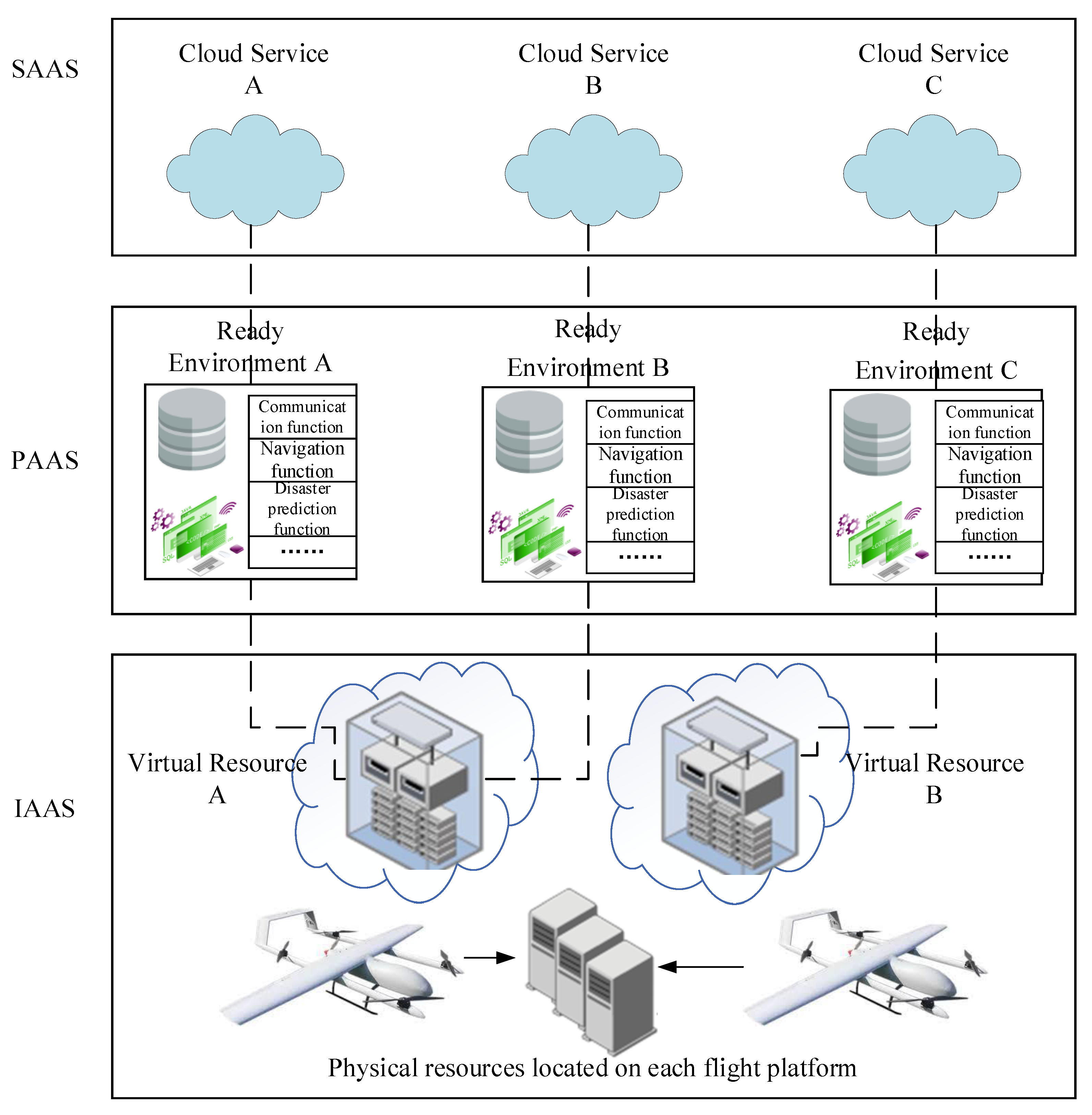
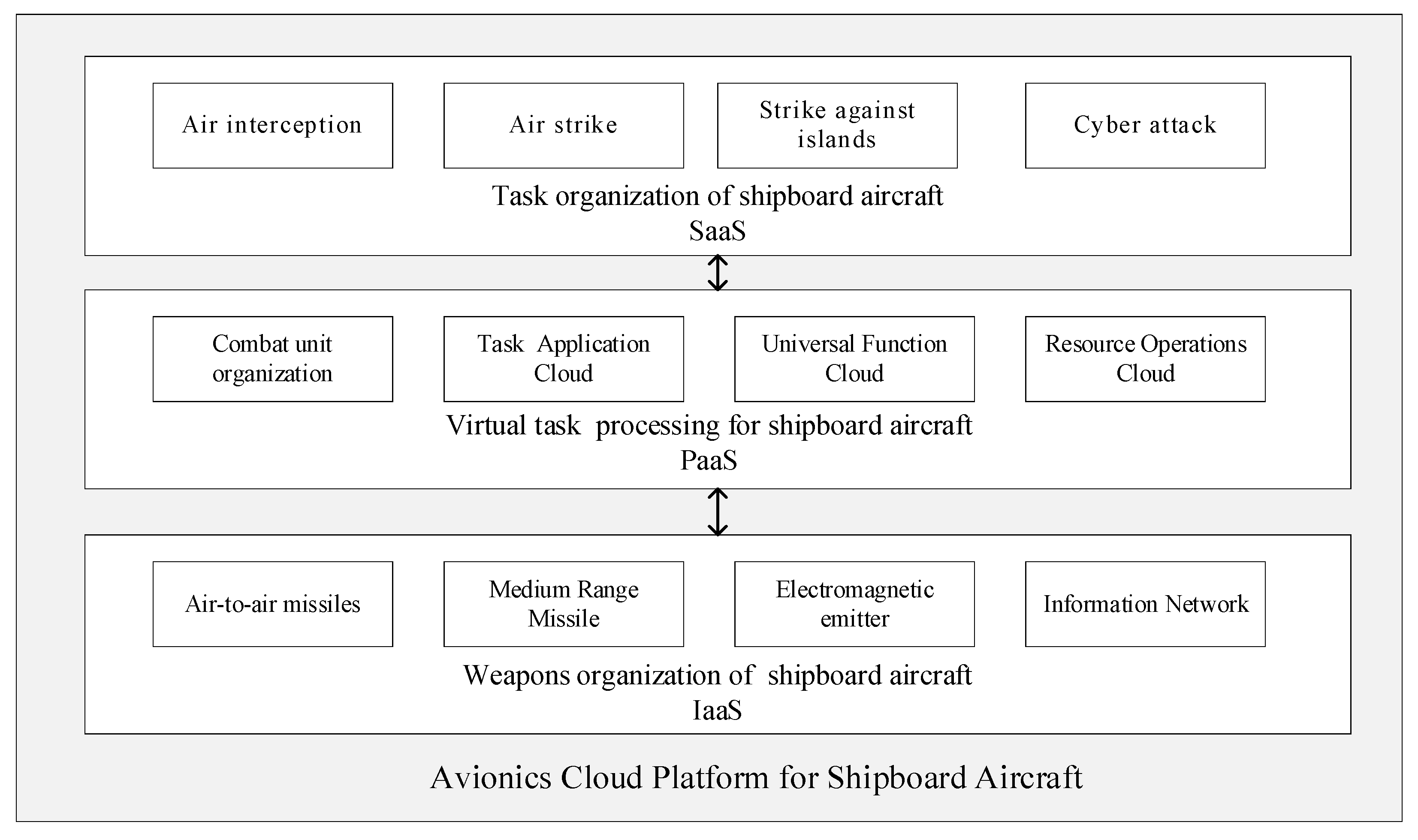
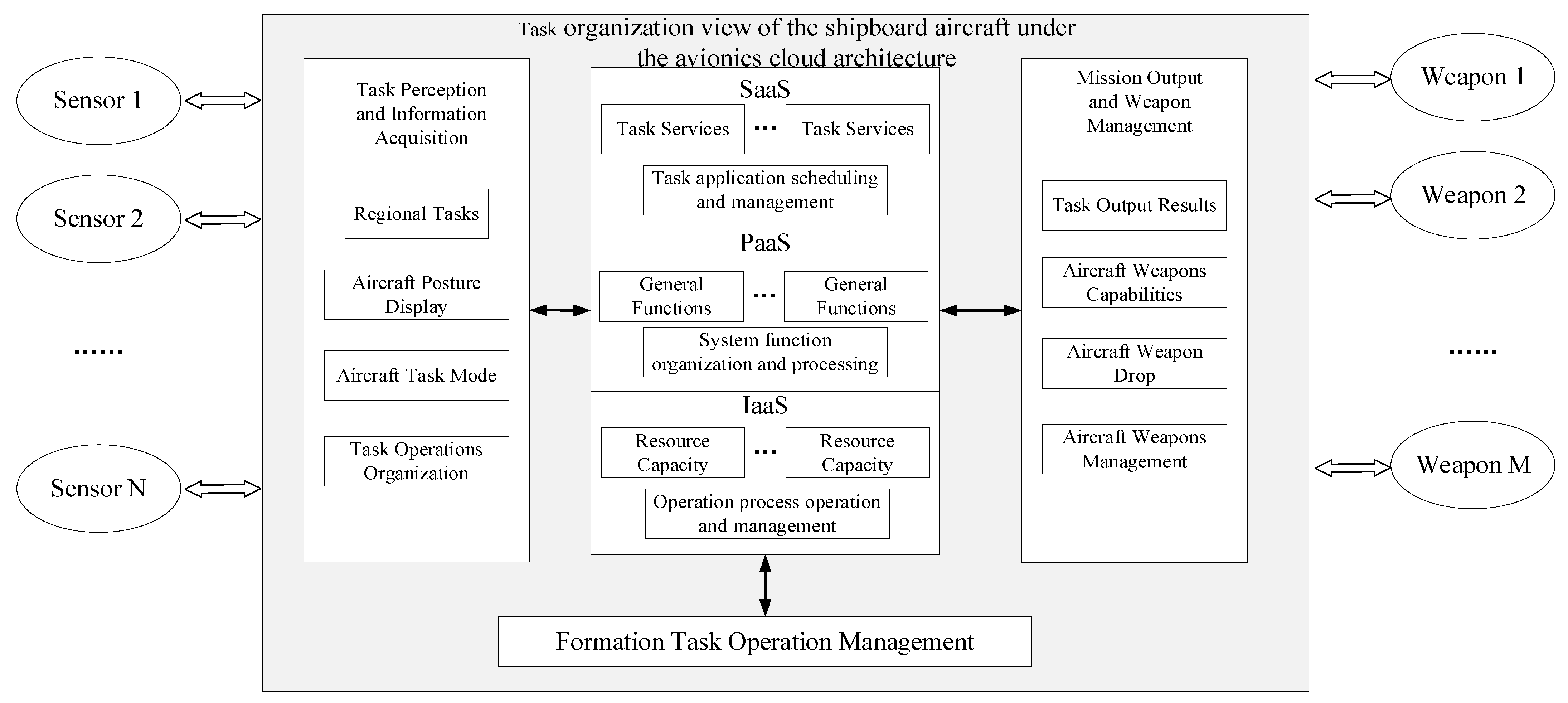
2.1. Avionics Cloud Organizational Structure
- (1)
- Application Cloud Platform (SaaS)
- (2)
- Function Cloud Platform (PaaS)
- (3)
- Resource Cloud Platform (IaaS)
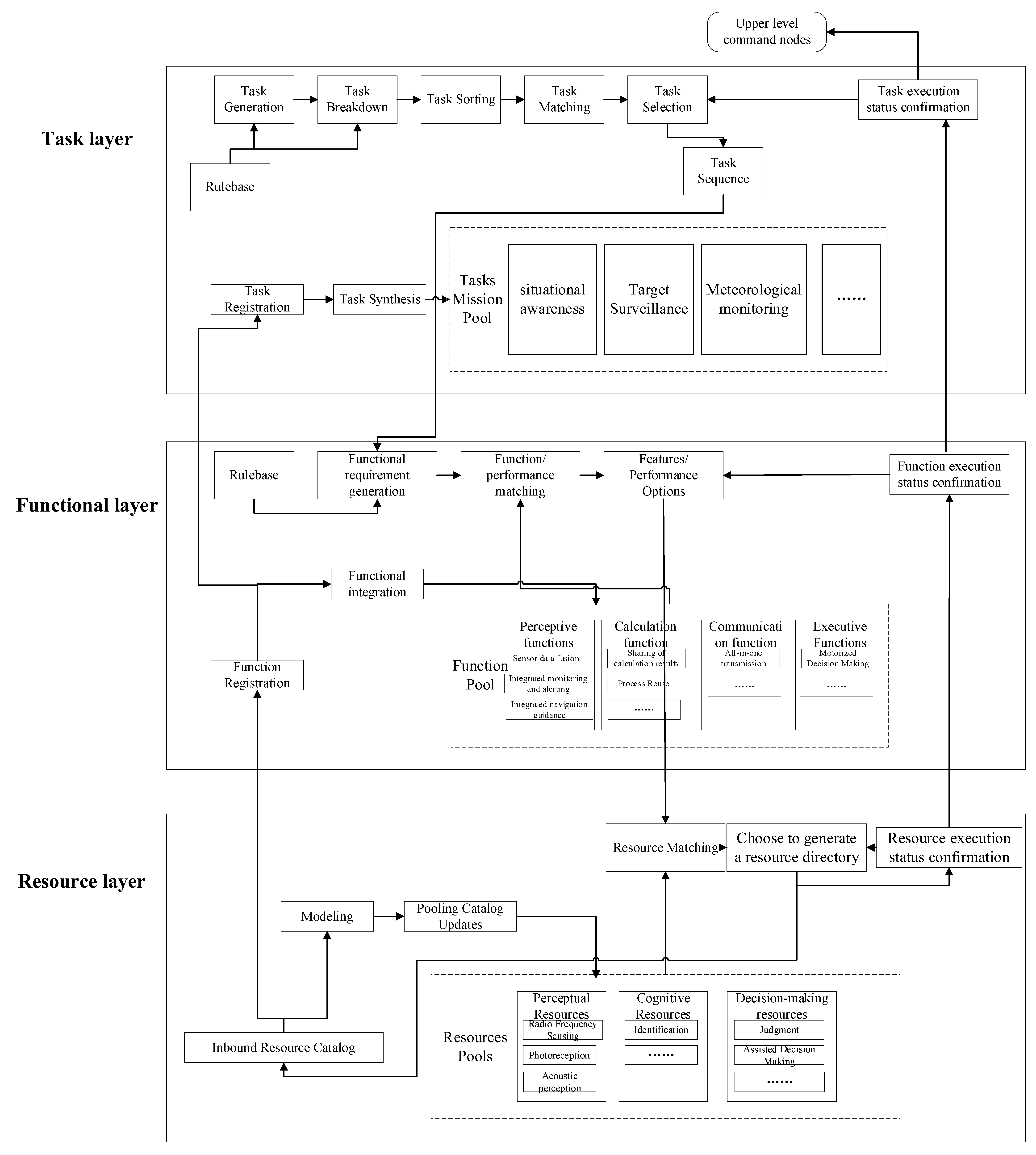
2.2. Avionics Cloud Logical Architecture
- (1)
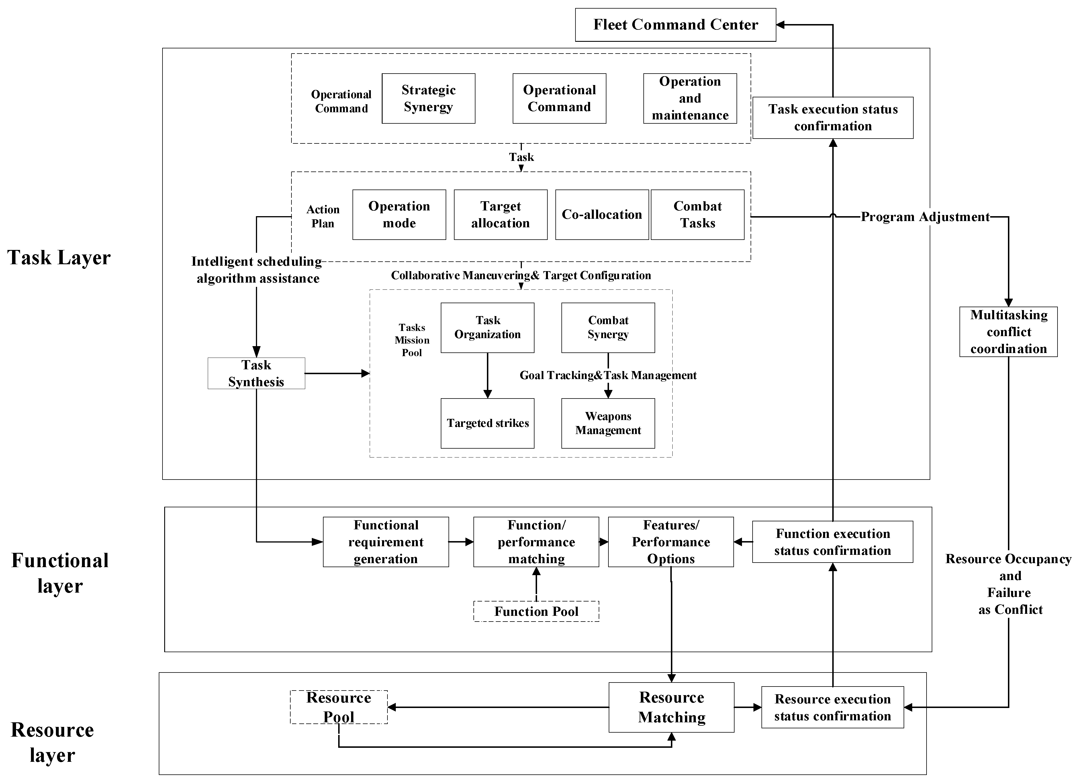
- Task layer
- (1)
- Based on the current functional cloud and resource cloud capabilities, the requirements are gradually decomposed into platforms with corresponding capabilities according to the requirements. In the task generation phase, the resource pool of the task cloud is the platform that can perform various tasks, and the platform that can be selected to meet the task requirements is selected from the current resource pool. The task is organized to ensure that the requirements can be met. In the process of organization, the process of how many platforms need to be selected from the resource pool and how to collaborate between platforms to generate plans is undertaken in the task cloud based on task dynamic demand elasticity.
- (2)
- Based on the task plan, a suitable sequence of units is selected to execute tasks in real-time based on the current platform operation status. In the task execution phase, based on the changes in demand caused by changes in the task plan and current scenario, as well as battle damage, etc., the platform is automatically increased or decreased from the resource pool to ensure that the demand is met. This means that the task execution can be completed automatically and flexibly during the execution process.
- (2)
- Functional layer
- (1)
- Task-oriented requirements and selection of available functions from the pool of functional resources. When, the function organization and fusion method meet the task capability requirements, this is called the function generation and organization phase. In this phase, facing the dynamic changes of the task, the functional cloud dynamically selects the required functions. In addition, based on the functional capability demand of real-time fusion to enhance the capability, the elasticity achieves dynamic function generation and organization.
- (2)
- Function execution is based on the current function’s required physical resource operation state, and real-time selection of the appropriate physical platform to execute the function, called function execution. In the functional execution phase, based on the functional organization and changes in demand caused by changes in the current scenario and battle damage, functional modules are automatically added or reduced from the resource pool to ensure that the capability requirements are met. This means that functional execution can be performed automatically and flexibly during the execution process.
- (3)
- Resource Layer
3. Problem Description
4. Algorithm Description
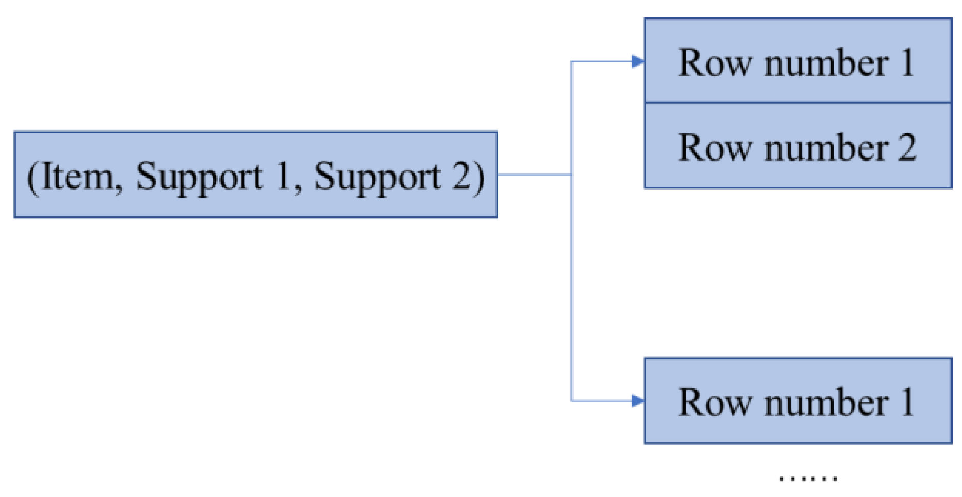
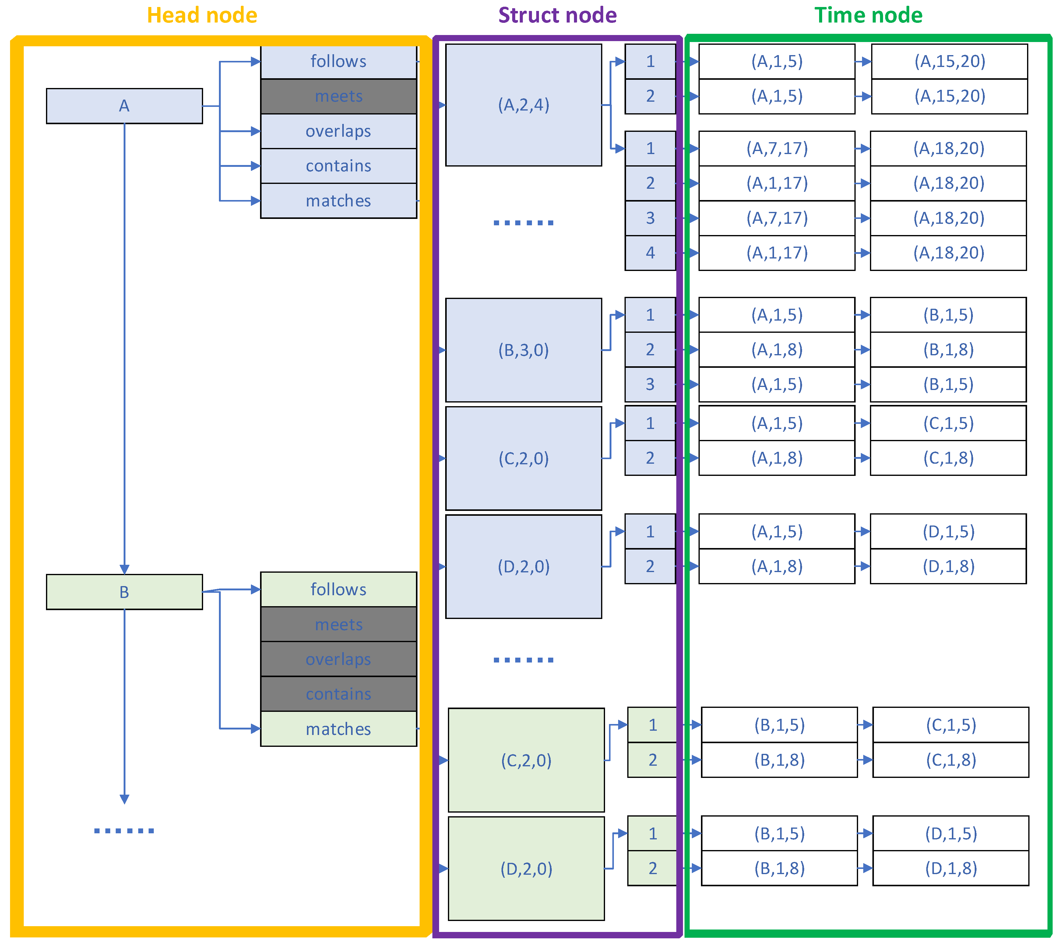
4.1. Data Structure
4.2. Pruning Strategy
4.3. DiMining Algorithm
| Algorithm 1 DiMining Algorithm |
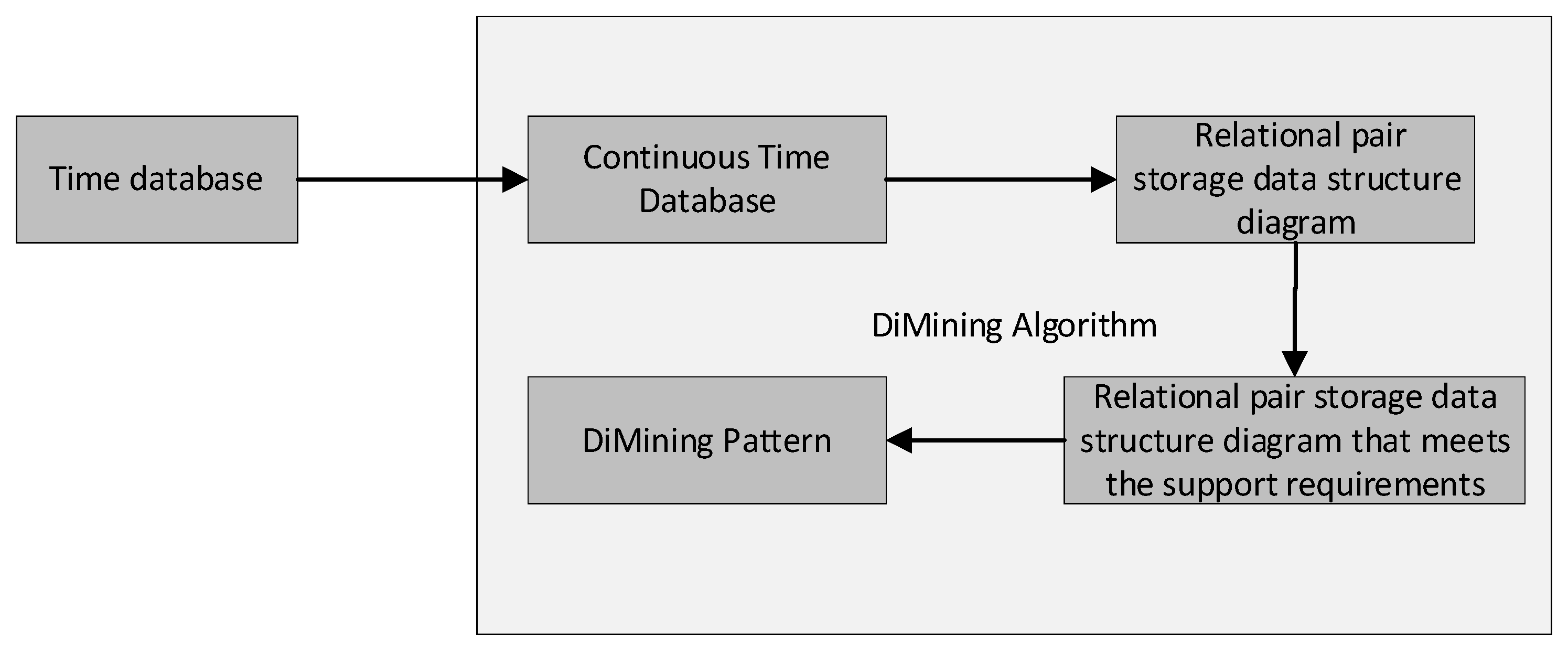
| Data: D1: high execution efficiency dataset, D2: low execution efficiency dataset , r: current extended subspace differential frequent pattern, R: relational pairs store data structures, constraints: predefined constraints ε. Result: Maximum differential frequent pattern set 1 ; ; ; ; 2 R ← getRelation (D1, D2); 3 for each rR do 4 if the SDF of the current relation meets the constraints then 5 Store current relation; 6 end if 7 flag ← growDiM(R, r, ); 8 if flag ==0 then 9 MSD←get_result(r); 10 end if 11 end for 12 return DiMining Pattern |
| Algorithm 2 getRelation (D1, D2) |
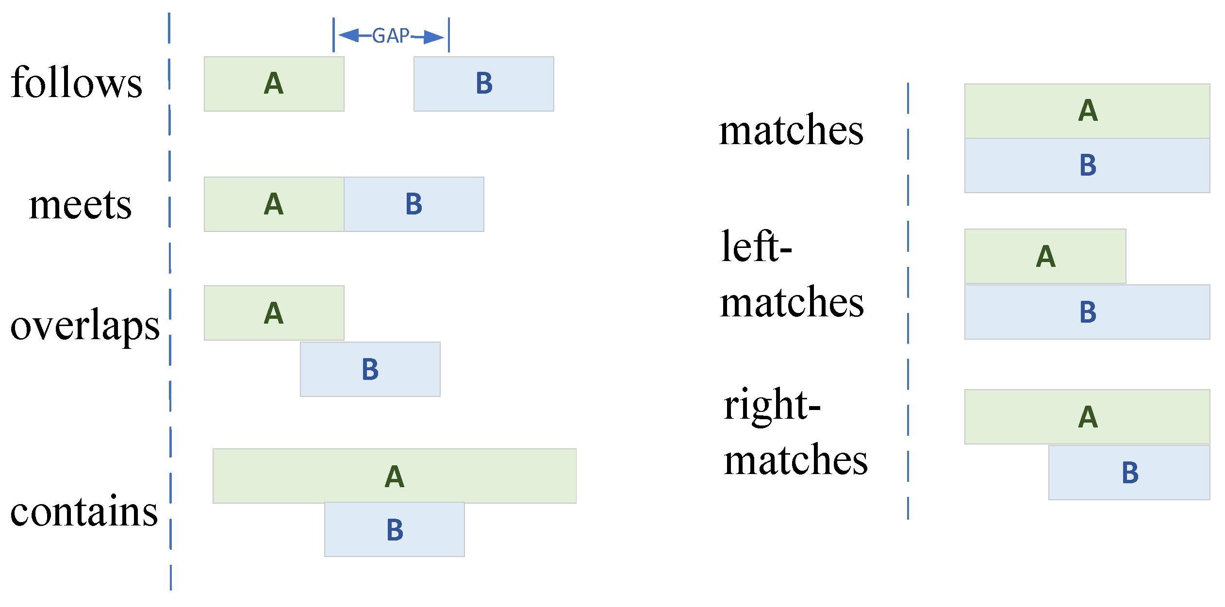
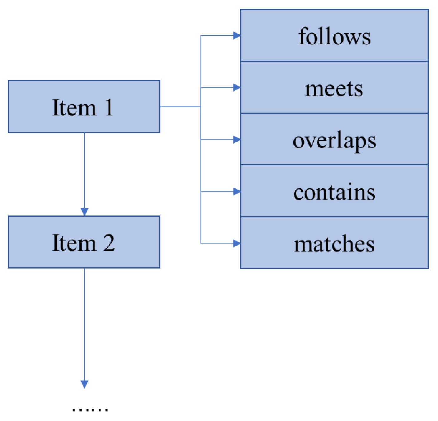
| Data: D1: high execution efficiency dataset, D2: low execution efficiency dataset. Result: R: relational pairs store data structures 1 for each I1, I2D1(or D2) do 2 if there is follows relationship between I1 and I2 then 3 I1.follows <- I2; 4 else if there is meets relationship between I1 and I2 then 5 I1. meets <- I2; 6 else if there is overlaps relationship between I1 and I2 then 7 I1. overlaps <- I2; 8 else if there is contains relationship between I1 and I2 then 9 I1. contains <- I2; 10 else if there is matches relationship between I1 and I2then 11 I1. matches <- I2; 12 end if 13 R ← get_head (I1.follows, I1. meets, I1. overlaps, I1. contains, I1. matches); 14 end for 15 get_tl(R); 16 return R |
| Algorithm 3 growDiM(R, r, ) |
| Data: R: relational pairs store data structures, r: current extended subspace differential frequent pattern, constraints: predefined constraints . Result: flag: Determine whether the current expansion node needs to continue linear expansion. 1 N ←getPrecursornode(R,r); 2 M←getCandidatenode(R,r); 3 if the set of transaction link 1 of PMiNj isn’t a subset of the set of transaction link 1 of PNj then 4 flag=0; 5 return flag 6 end if 7 if the maximum binomial subset support of PMiNj in dataset 2 is less than the maximum binomial subset support of PNj then 8 flag=0; 9 return flag 10 end if 11 if PMiNj is not a differential frequent pattern then 12 flag=0; 13 return flag 14 end if 15 flag=1; 16 return flag |
5. Experiment and Analysis
5.1. Efficiency Comparison
- (1)
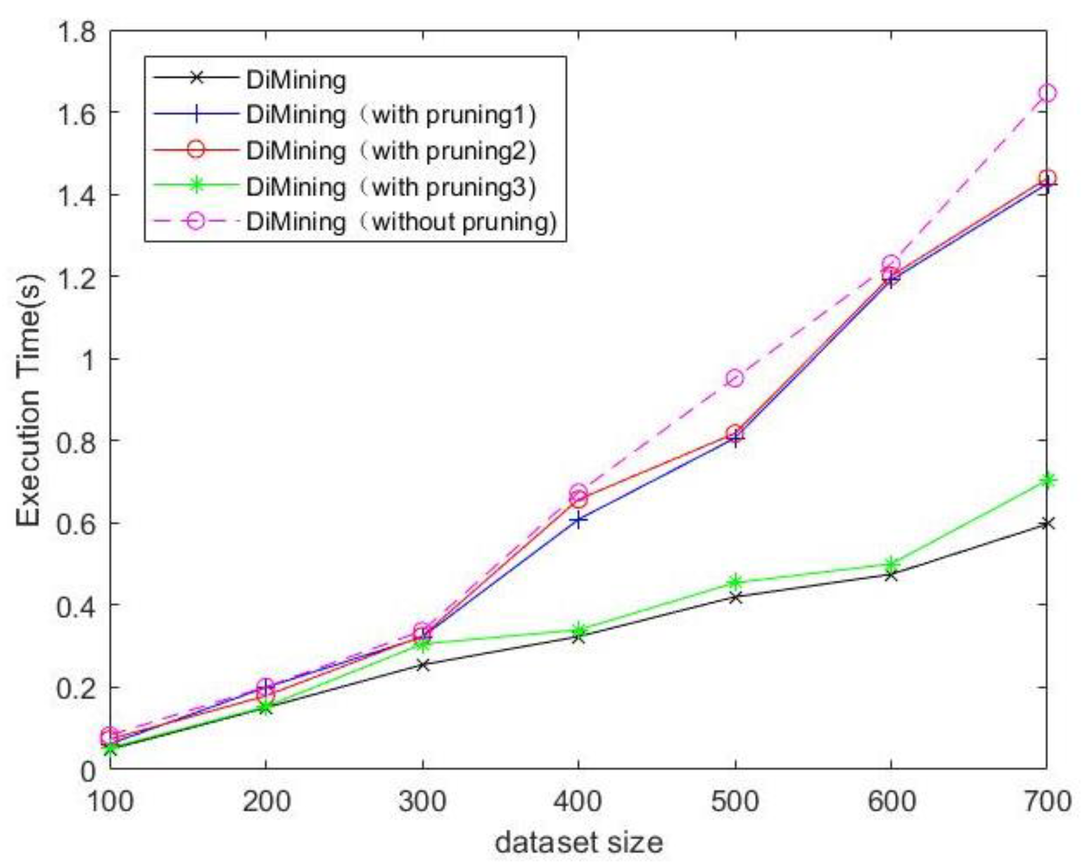
- Pruning strategy analysis
- (2)
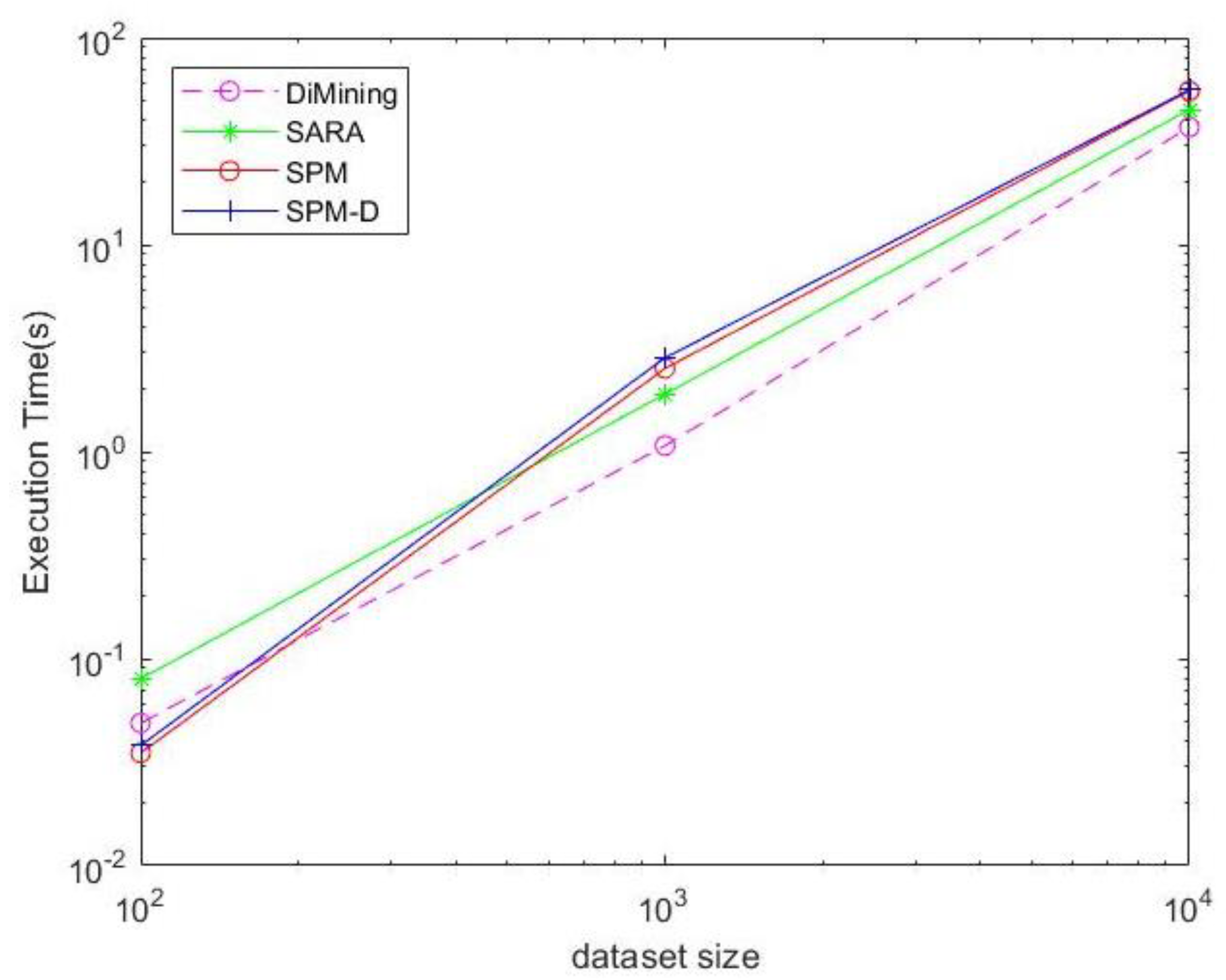
- Efficiency comparison
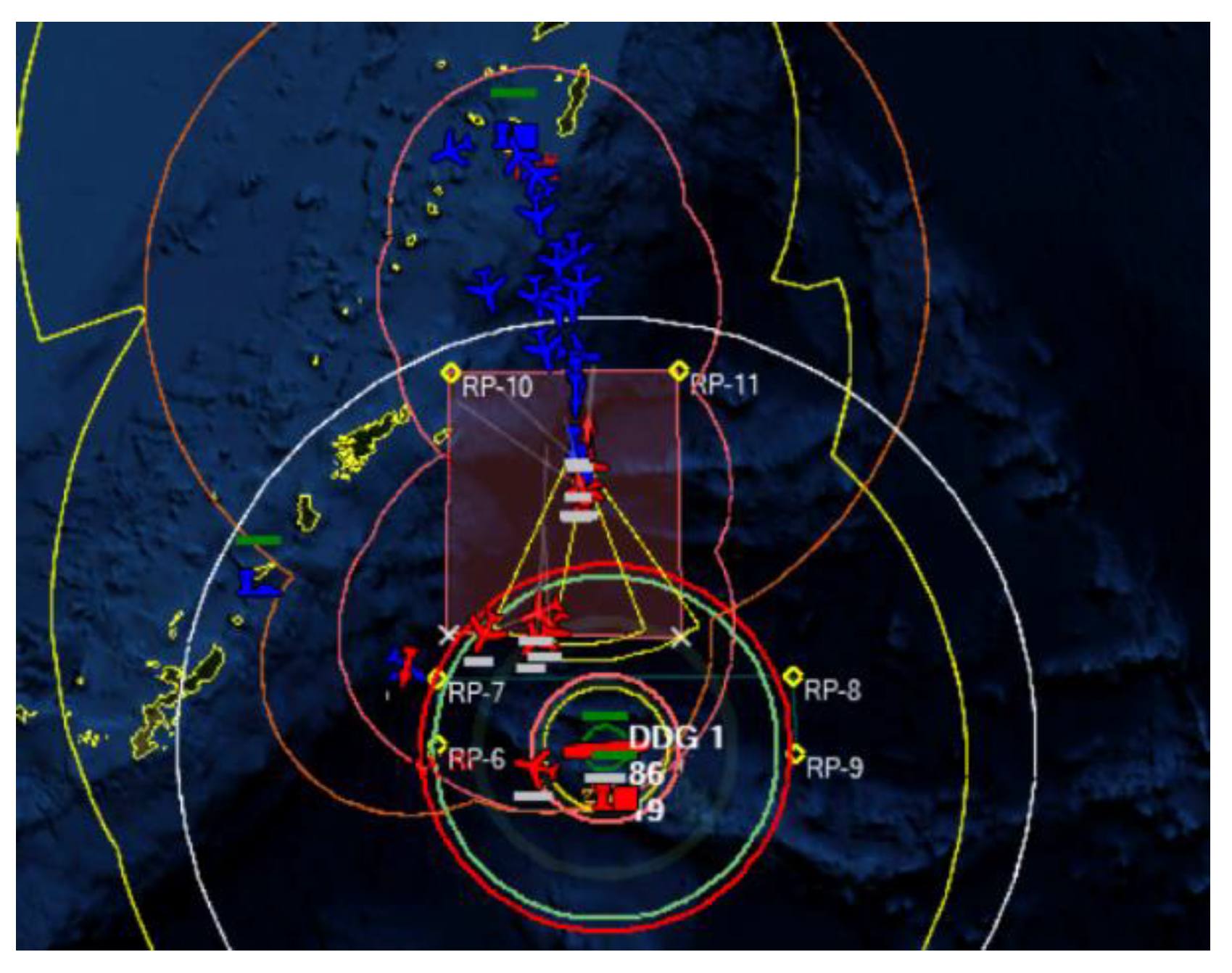
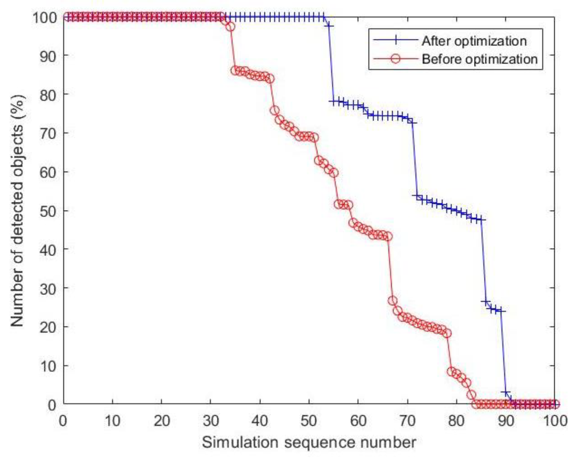
5.2. Simulation Experiment
6. Conclusions
Author Contributions
Funding
Data Availability Statement
Conflicts of Interest
References
- Mark, H.; George, V.; Gregary, B.P. A comparison of open architecture standards for the development of complex military systems: GRA, FACE, SCA NeXT (4.0). In Proceedings of the MILCOM 2012–2012 IEEE Military Communications Conference, Orlando, FL, USA, 29 October–1 November 2012. [Google Scholar]
- Guertin, N. How the navy is using open systems architecture to revolutionize capability acquisition. In Proceedings of the 12th Annual Acquisition Research Symposium, Monterey, CA, USA, 13–14 May 2015. [Google Scholar]
- Du, X.; Du, C.; Chen, J.; Liu, Y. An energy-aware resource allocation method for avionics systems based on improved ant colony optimization algorithm. Comput. Electr. Eng. 2023, 105, 108515. [Google Scholar] [CrossRef]
- Elkholy, W.; El-Menshawy, M.; Bentahar, J.; Elqortobi, M.; Laarej, A.; Dssouli, R. Model checking intelligent avionics systems for test cases generation using multi-agent systems. Expert Syst. Appl. 2020, 156, 113458. [Google Scholar] [CrossRef]
- Kabashkin, I.; Filippov, V. Reliability of Software Applications in Integrated Modular Avionics. Transp. Res. Procedia 2020, 51, 75–81. [Google Scholar] [CrossRef]
- The Open Group. Technical Standard for Future Airborne Capability Environment (FACETM). Edition 2.1. Available online: http://www.opengroup.org/bookstore (accessed on 20 November 2019).
- Turiak, M.; Sedláčková, A.N.; Novak, A. Portable electronic devices on board of airplanes and their safety impact. In Telematics-Support for Transport, Proceedings of the 14th International Conference on Transport Systems Telematics, TST 2014, Katowice/Kraków/Ustroń, Poland, 22–25 October 2014; Springer: Berlin/Heidelberg, Germany, 2014. [Google Scholar] [CrossRef]
- Yang, H.; Sun, Y. A combination method for integrated modular avionics safety analysis. Aircr. Eng. Aerosp. Technol. 2022, 95, 345–357. [Google Scholar] [CrossRef]
- Dong, X.; Wang, M.; Liu, Y.; Xiao, G.; Huang, D.; Wang, G. An Efficient Spatial High Utility Occupancy Frequent Item Mining Algorithm for Task System Integration Architecture Design using MBSE Method. Aerosp. Syst. 2022, 5, 377–392. [Google Scholar] [CrossRef]
- Li, Z.; Li, Q.; Xiong, H. Avionics clouds: A generic scheme for future avionics systems. In Proceedings of the 2012 IEEE/AIAA 31st Digital Avionics Systems Conference (DASC), Williamsburg, VA, USA, 14–18 October 2012; pp. 6E4-1–6E4-10. [Google Scholar] [CrossRef]
- Nguyen, A.-Q.; Amrhar, A.; Landry, R. Direct RF Sampling Avionics Architecture for future multi-system integrated Avionics. In Proceedings of the 2018 16th IEEE International New Circuits and Systems Conference (NEWCAS), Montreal, QC, Canada, 24–27 June 2018; pp. 61–65. [Google Scholar] [CrossRef]
- Jianchun, X.; Zhonghua, W.; Yahui, L. The Distributed Computing Framework Research for Avionics Cloud. In Proceedings of the 2018 International Conference on Networking and Network Applications (NaNA), Xi’an, China, 12–15 October 2018; pp. 390–393. [Google Scholar] [CrossRef]
- Ma, X.; Jiang, C.; Huang, C. Cloud Task Optimization Scheduling based on Three-branch clustering. Comput. Sci. 2022, 49, 875–881. [Google Scholar]
- Ye, F.; Shen, W. Task scheduling algorithm based on depth of reinforcement learning to improve. J. Comput. Age 2022, 11, 58+55–64. [Google Scholar]
- Wang, S.; Sun, J.; Wang, P.; Yang, A. Cloud and synergy of resource scheduling optimization. J. Telecom Sci. 2022, 12, 1–9. [Google Scholar]
- Fournier-Viger, P.; Nkambou, R.; Mephu Nguifo, E. A Knowledge Discovery Framework for Learning Task Models from User Interactions in Intelligent Tutoring Systems. In Proceedings of the 7th Mexican International Conference on Artificial Intelligence (MICAI 2008), Atizapan de Zaragoza, Mexico, 27–31 October 2008; Springer: Berlin/Heidelberg, Germany, 2008; pp. 765–778. [Google Scholar]
- Huang, J.-W.; Jaysawal, B.P.; Chen, K.-Y.; Wu, Y.-B. Mining frequent and top-K High Utility Time Interval-based Events with Duration patterns. Knowl. Inf. Syst. 2019, 61, 1331–1359. [Google Scholar] [CrossRef]
- Ritika; Gupta, S. K. HUFTI-SPM: High-utility and frequent time-interval sequential pattern mining from transactional databases. Int. J. Data Sci. Anal. 2022, 13, 239–250. [Google Scholar] [CrossRef]
- Mordvanyuk, N.; Lopez, B.; Bifet, A. vertTIRP: Robust and efficient vertical frequent time interval-related pattern mining. Expert Syst. Appl. 2021, 168, 114276. [Google Scholar] [CrossRef]
- Lee, Z.; Lindgren, T.; Papapetrou, P. Z-Miner: An Efficient Method for Mining Frequent Arrangements of Event Intervals. In Proceedings of the 26th ACM SIGKDD International Conference on Knowledge Discovery & Data Mining (KDD ‘20), New York, NY, USA, 6–10 July 2020; pp. 524–534. [Google Scholar]
- Fang, G.; Kuang, R.; Pandey, G.; Steinbach, M.; Myers, C.L.; Kumar, V. Subspace Differential Co-expression Analysis: Problem Definition and A General Approach. In Proceedings of the 15th Pacific Symposium on Biocomputing (PSB), Kamuela, HI, USA, 4–8 January 2010; Volume 15, pp. 145–156. [Google Scholar]


| Number of T | Data |
|---|---|
| T1 | (A, 1, 5) (B, 1, 5) (C, 1, 5) (D, 1, 5) (B, 7, 13) (A, 15, 20) |
| T2 | (A, 1, 8) (B, 1, 8) (C, 1, 8) (D, 1, 8) (A, 15, 20) |
| T3 | (A, 1, 5) (B, 1, 5) (C, 7, 13) (B, 15, 20) |
| T4 | (A, 1, 17) (D, 9, 11) (C, 11, 13) (D, 14, 18) (B, 18, 20) |
| Number of T | Data |
|---|---|
| T1 | (B, 1, 8) (A, 7, 17) (D, 9, 11) (C, 10, 12) (D, 14, 18) (A, 18, 20) |
| T2 | (A, 1, 17) (D, 9, 11) (C, 10, 12) (D, 14, 18) (A, 18, 20) |
| T3 | (A, 7, 17) (C, 9, 13) (D, 12, 14) (C, 14, 18) (A, 18, 20) |
| T4 | (A, 1, 17) (C, 11, 13) (D, 12, 14) (C, 14, 18) (A, 18, 20) |
| Task Number | Task Name |
|---|---|
| F1 | UAV anti-radiation Task |
| F2 | Early Warning Aircraft Radar 1 Detection Task |
| F3 | Early Warning Aircraft Radar 2 Detection Task |
| F4 | UAV Radar 1 Detection Task |
| F5 | UAV Radar 2 Detection Task |
| F6 | UAV Radar 3 Detection Task |
| F7 | UAV Radar 4 Detection Task |
| Number | Result |
|---|---|
| 1 | F1 f F2 o F4 |
| 2 | F2 f F2 o F4 |
| 3 | F4 f F5 o F5 |
| 4 | F4 f F5 |
| 5 | F4 m F7 |
| 6 | F4 a F2 o F4 |
| 7 | F5 c F5 |
Disclaimer/Publisher’s Note: The statements, opinions and data contained in all publications are solely those of the individual author(s) and contributor(s) and not of MDPI and/or the editor(s). MDPI and/or the editor(s) disclaim responsibility for any injury to people or property resulting from any ideas, methods, instructions or products referred to in the content. |
© 2023 by the authors. Licensee MDPI, Basel, Switzerland. This article is an open access article distributed under the terms and conditions of the Creative Commons Attribution (CC BY) license (https://creativecommons.org/licenses/by/4.0/).
Share and Cite
Dong, X.; Wang, X.; Peng, L.; Wang, M.; Wang, G. An Efficient Task Synthesis Method Based on Subspace Differential Patterns for Arrangements of Event Intervals Mining in the Avionics Cloud System Architecture. Aerospace 2023, 10, 249. https://doi.org/10.3390/aerospace10030249
Dong X, Wang X, Peng L, Wang M, Wang G. An Efficient Task Synthesis Method Based on Subspace Differential Patterns for Arrangements of Event Intervals Mining in the Avionics Cloud System Architecture. Aerospace. 2023; 10(3):249. https://doi.org/10.3390/aerospace10030249
Chicago/Turabian StyleDong, Xiaoxu, Xin Wang, Ling Peng, Miao Wang, and Guoqing Wang. 2023. "An Efficient Task Synthesis Method Based on Subspace Differential Patterns for Arrangements of Event Intervals Mining in the Avionics Cloud System Architecture" Aerospace 10, no. 3: 249. https://doi.org/10.3390/aerospace10030249