Article

RAMSEES: A Model of the Atmospheric Radiative Environment Based on Geant4 Simulation of Extensive Air Shower

1
Environnement and New Components Section, Centre National d’Études Spatiales (CNES), 31400 Toulouse, France
2
Radiation Engineering Department, Tests and Radiations (TRAD), 31670 Labège, France
3
Institut d’Électronique et des Systèmes, UMR-CNRS 5214, University of Montpellier, 34095 Montpellier, France
*
Authors to whom correspondence should be addressed.
Aerospace 2023, 10(3), 295; https://doi.org/10.3390/aerospace10030295
Submission received: 31 January 2023 / Revised: 9 March 2023 / Accepted: 14 March 2023 / Published: 16 March 2023
(This article belongs to the Collection Avionic Systems)

Abstract

:
The device downscaling of electronic components has given rise to the need to consider specific failures in onboard airplane electronics. Single Event Effects (SEE) are a kind of failures that occur due to radiation in the atmosphere. For the purpose of ensuring onboard electronic reliability, there is a clear need for new tools to predict the SEE rate, at both avionic altitudes and at ground level. In this work, we develop a new tool: RAMSEES (Radiation Atmospheric Model for SEE Simulation), which simulates the atmospheric radiative environment induced by cosmic rays. This multiscale and multi-physics phenomenon is simulated using the Geant4 toolkit, allowing the creation of a database to characterize the radiation environment in the atmosphere as a function of altitude. We show the need to simulate very high-energy particles such as 100 TeV space protons, because they are the main contributor of radiation at avionic altitudes as well as at ground level. Our approach shows a good agreement with the experimental data, the standards, and other models, and it also points out some discrepancies, especially below 18 km of altitude. RAMSEES can be the basis of the estimation of the SEE rate from ground level to the stratosphere, at any given position and time.

1. Introduction

The Earth’s magnetic field traps a lot of the particles coming from outer space, creating the radiation belts, also called Van Allen Belts [1]. However, the highest energetic particles, the Galactic Cosmic Rays (GCR), can go through the magnetospheric shielding and reach the Earth’s atmosphere. The GCR interact with the atmosphere constituents, creating the so-called Extensive Air Shower (EAS) [2,3,4]. An EAS is a physical phenomenon taking place when a primary particle coming from space interacts with the Earth’s atmosphere. The single primary particle generates a zoo of secondary particles: neutron, electron, photon, muon. These secondary particles will interact with the atmospheric atoms, generating new secondary particles in a shower of particles, which will lead to the creation of the atmospheric radiative environment.
Many works have already dealt with radiation in the atmosphere [5,6,7,8,9]. They all have their targeted applications (e.g., knowledge of the environment, cosmic rays study, dosimetry for aircrew), their limitations and are generally not easy to be transposed from one application to another. In this work, our targeted application is radiation-induced failures in microelectronics. For a long time, the Radiation Hardness Assurance (RHA) for microelectronics or the safety issue created by the atmospheric radiative environment was not addressed because the risk induced was estimated to be too low. The atmospheric radiative environment induces mostly one kind of RHA risk: the Single Event Effect (SEE). An SEE appears when a single particle—generally a heavy ion, a neutron, or a proton— induces a failure in an electronic device. This kind of risk is assessed in satellites because they are designed to be resistant to space radiation-induced failures; however, airplanes were initially not so designed. In the early 90’s, after several unexpected electronic failures in flight, a collaboration between IBM (International Business Machines Corporation, Armonk, NY, USA) and Boeing lead to the conclusion that these errors were due to radiation-induced SEE at avionic altitude, changing the status of radiation-induced failures in avionics from a myth to a proven scientific reality [10,11]. Following those events, a major interest in that field of study was born in the scientific community. It led to one standard for the ground electronics based on a neutron flux at New York “JEDEC” [12], a standard for airplanes at 12 km of altitude “IEC” [13], and two models of the atmospheric radiative environment: “MAIRE+” (Models for Atmospheric Ionizing Radiation Effects) [14] and “EXPACS” (Excel-based Program for calculating Atmospheric Cosmic-ray Spectrum) [15].
The JEDEC standard gives atmospheric neutron flux at New York City, USA at sea level as a reference and a formula to adapt it to any location. It is based on Ziegler’s work on cosmic rays [16] and the NASA-Langley neutron flux model. In the case of IEC, the standard is the neutron flux at 12 km altitude at 45° of latitude and can be adapted to any location. The IEC model is based on a fit of the AMES data, a NASA experiment of the 70’s, measuring the atmospheric neutrons. The MAIRE+ model, which is a new version of MAIRE [17] and QARM (QinetiQ Atmospheric Radiation Model) [18,19], based on a Monte Carlo simulation of the interactions of cosmic rays with the atmosphere via MCNPX (Monte Carlo N-Particle eXtended) [20]. Developed by the Surrey Space Center to provide real-time information to the airline industry about the radiation dose received by crew and passengers, it is logically focused on the Dose rate. Moreover, EXPACS was developed by the JAEA (Japan Atomic Energy Agency) [21,22,23,24]. It is based on EAS simulation performed by PHITS (Particle and Heavy Ion Transport Code System) [25] a homemade Monte Carlo code. It provides the effective dose, ambient dose equivalent and absorbed dose in air based on the atmospheric cosmic-ray spectra. These tools were created in the early 2000s following the work of Normand and Taber [10,11]. In the case of EXPACS and MAIRE+, they have been updated and upgraded until today.
Moreover, with transistor sizes shrinking, we have observed an increase in the sensitivity of electronic components to radiations. One example was revealed during the CONCORDIASI scientific balloon campaign at Concordia, Antarctica in 2010, when hundreds of anomalies were recorded because a commercial electronic device sensible to Single Event Latch up (SEL) was on board [26]. In such cases, it becomes important to qualify the reliability of the electronic devices in the atmospheric radiative environment. The RHA became a topic discussed in a bigger community and the need of a precise model to make calculations of failure rate at all the levels of the atmosphere is now higher than ever before.
Here, we present a new model based on a Monte Carlo simulation with state-of-the-art data as input and state-of-the-art Monte Carlo tools based on Geant4 [27,28,29], a toolkit developed by CERN (European Organization for Nuclear Research). Even if some other tools exist, they are not fully satisfactory, as they do not allow us to implement all the ingredients required to address our concerns with microelectronic reliability. On the contrary, the use of a toolkit such as Geant4 is ideal and will, in future work, allow us to consider more complex simulations that include, for example, the effect of the nature of the ground, the presence of buildings or the effect of aircraft materials. Our model, based on technology and scientific knowledge, is designed to allow a better RHA at every altitude of the atmosphere and a better reliability of the electronic devices, especially for ground, avionic and balloon applications.
This paper starts with a description of our approach to model the atmospheric radiative environment. Then, we present the parameters needed to simulate an EAS, which are the structure of the atmosphere and the primary particle spectrum. Afterwards, we present our method to model the EAS phenomenon via a Monte Carlo simulation. Subsequently, we present a comparison of our results with experimental data and then with the standards and other models. Finally, we conclude this paper by presenting our tool RAMSEES (Radiation Atmospheric Model for Single Event Effect Simulation) and its fields of application.

2. Approach and Methodology

Our objective in creating RAMSEES was to give a user-friendly tool, which allows the evaluation of the spectrum of secondary particles anywhere and anytime on the planet, allowing users to calculate the SEE number and predict the risks for their flight, their launch, or ground application.

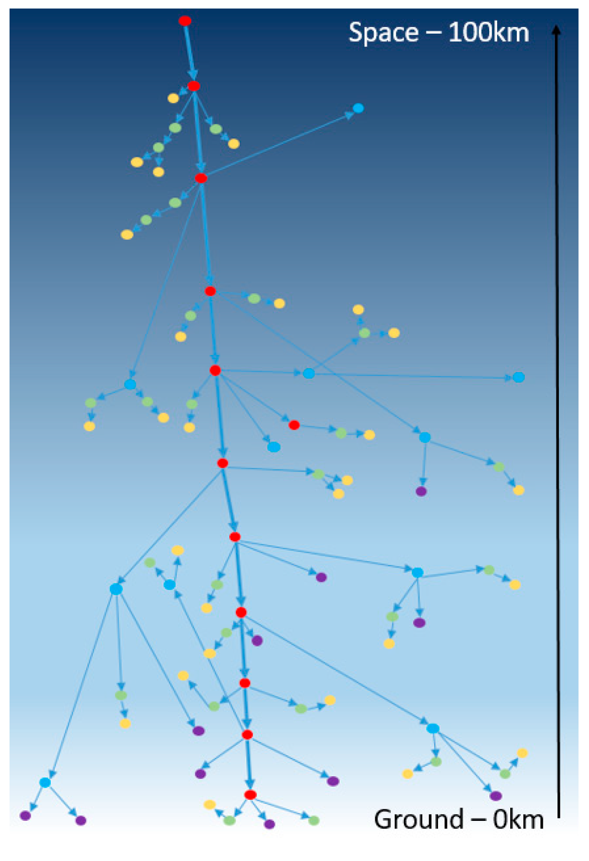
2.1. Extensive Atmospheric Air Shower

An Extensive Atmospheric Shower (EAS) is the physical phenomenon created by high-energy particles coming from space when they enter the top of atmosphere [2,3]. During their propagation in the atmosphere, these primary particles interact with air molecules and create secondary particles, which themselves continue to interact with the atmosphere, generating new secondaries and creating showers of particles. This process will continue until no more interactions are possible. In Figure 1, a schematic of an EAS is presented, showing the creation of secondary particles from a primary particle.

2.2. Approach in Modelling the EAS Phenomenon

To give the user a tool able to calculate SEE, we divided the work into four steps, presented in Figure 2. The first one is the collection of the information needed to simulate the EAS phenomenon, which are the primary particles—in our case, the protons coming from space—and the atmosphere definition. The second one is the choice of the physics used to simulate the EAS; in our case, the Monte Carlo simulation by Geant4 using the QGSP_BERT physics list. The third one is the EAS modelling itself, representing the geometry and simulating enough time to gather sufficient statistics. We simulated the EAS phenomenon in the CNES (Centre National d’Études Spatiales) Cluster during 100,000 h equivalent on one CPU using our C++ code with the Geant4 toolkit. The fourth one is the compilation of the simulation. We combined all the calculations, i.e., 350,000 simulations, for more than 1.2 TB of data by using Python and the Django framework. Finally, we developed our tool, which includes a database of the EAS interaction in the atmosphere, allowing particle spectra to be estimated for any place on Earth.

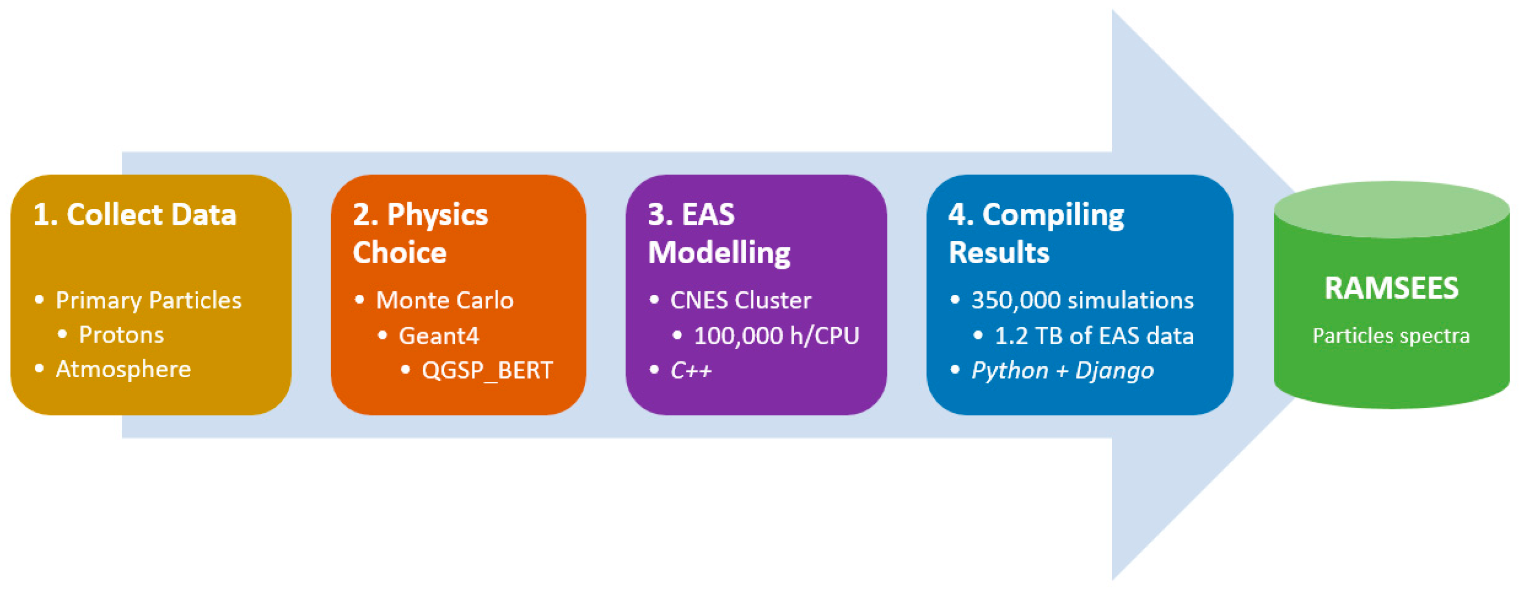
2.3. Physics and Methodology

Figure 3 is a schematic of the principle behind our simulation. We simulated showers of particles in a volume of atmosphere of 30 km × 30 km × 100 km. Primary protons are incoming at the top of the atmosphere and their energies are chosen according to Section 3.2.2. For the sake of simplicity, we consider that protons reach the atmosphere with a normal incidence (i.e., vertically). Doing so implies that the flux of primary protons is fully described by the quantity d ϕ i n c d E i n c as we integrated over the solid angle. Moreover, the density of the atmosphere varies, as explained in Section 3.1.2. At different altitudes, noted z, we simulated a planar detector to track secondary particles involved in an EAS. Such a detector provides d N i d E i z , the differential number of particles i, with energy Ei, which can be created by a primary proton at an altitude z. Then, we can calculate the differential flux of that kind of particle at the altitude of the detector:
d ϕ i d E i z = 2 π d N i d E i z · d ϕ i n c d E i n c d E i n c
The methodology to compute particle spectra is the following:
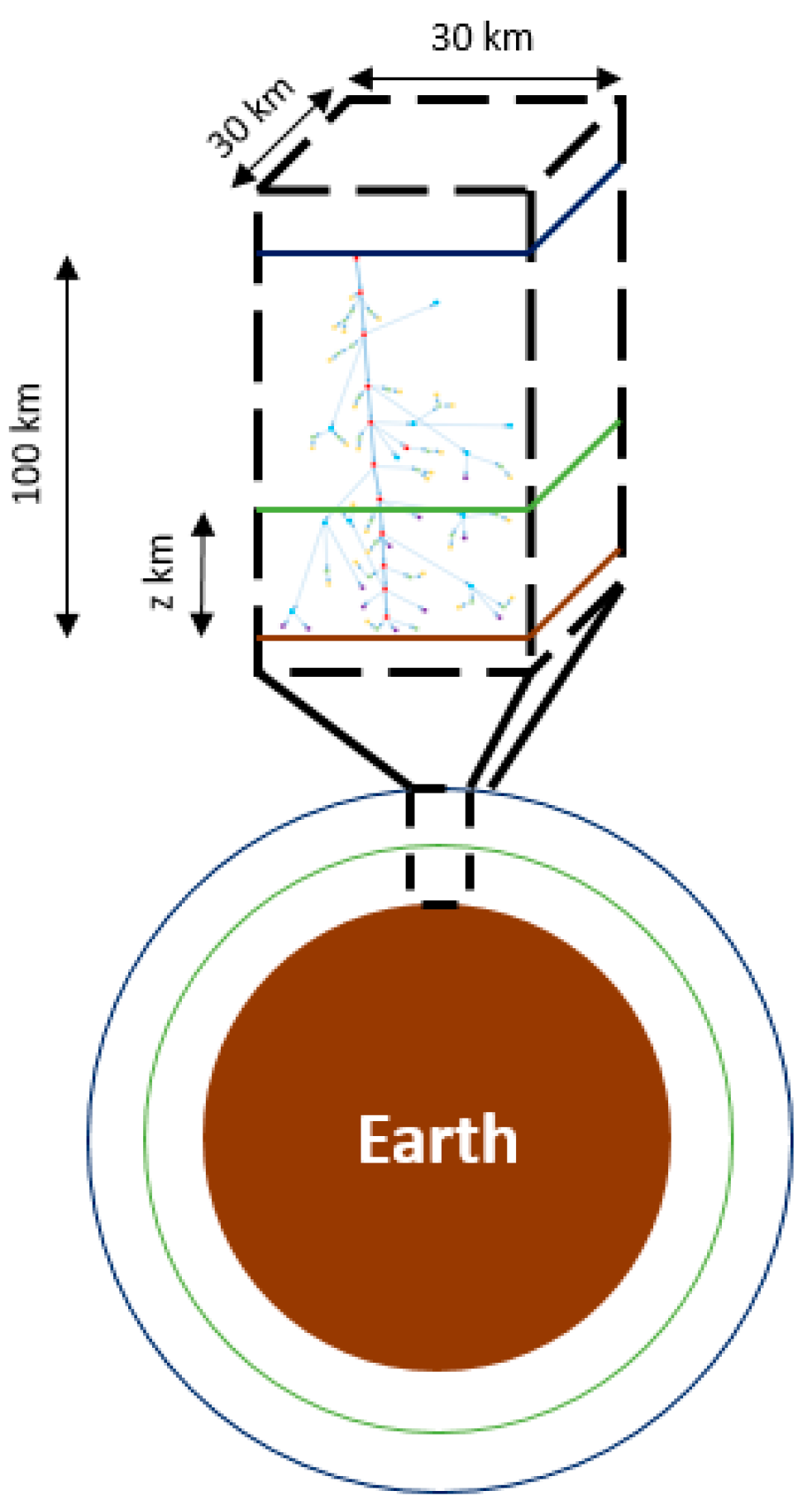
  • We create a planar detector in the atmosphere at the altitude z . From this detector, we can extract every particle crossing it and then extract all the secondaries generated by the primary particle.
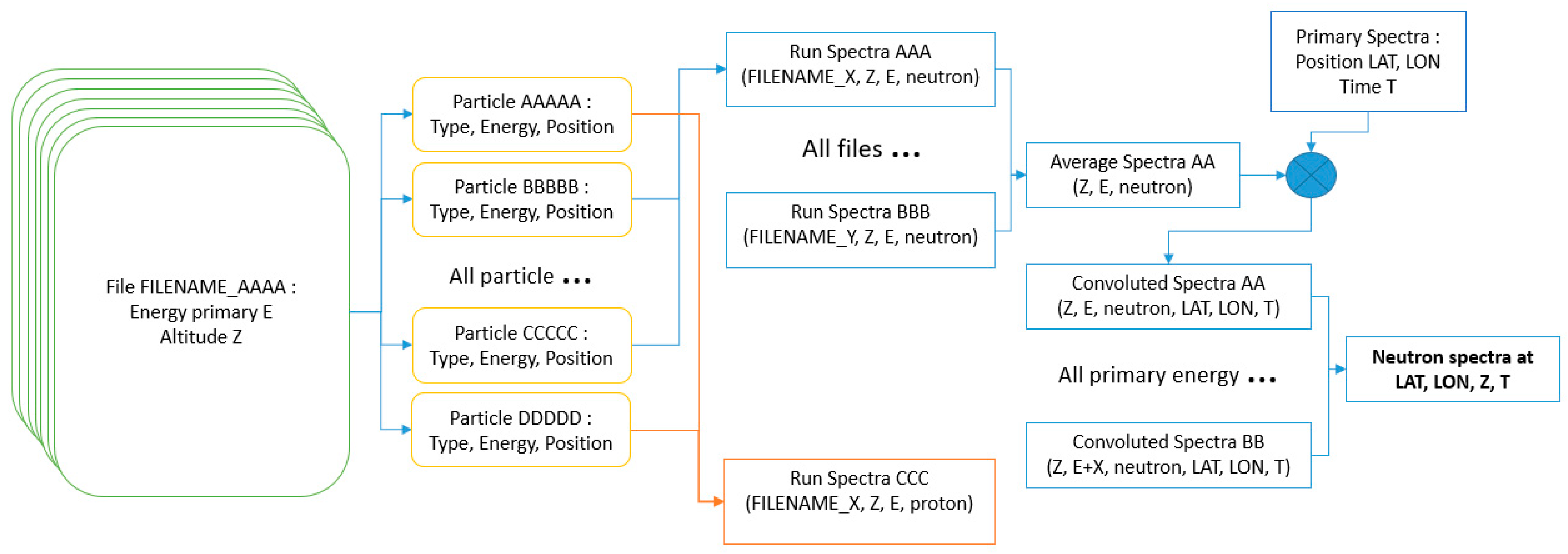
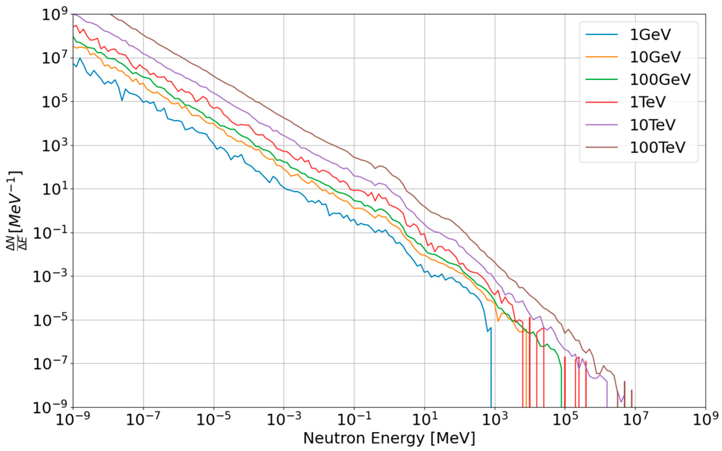
  • By compiling all the particles generated by type (neutron, proton, muons…) we create a spectrum for each kind of particle i .
  • Then we compile all the spectra of the particles i generated by all simulations of a primary of the same energy E at the same altitude z to create the average spectra generated by a primary of energy E at the altitude z .
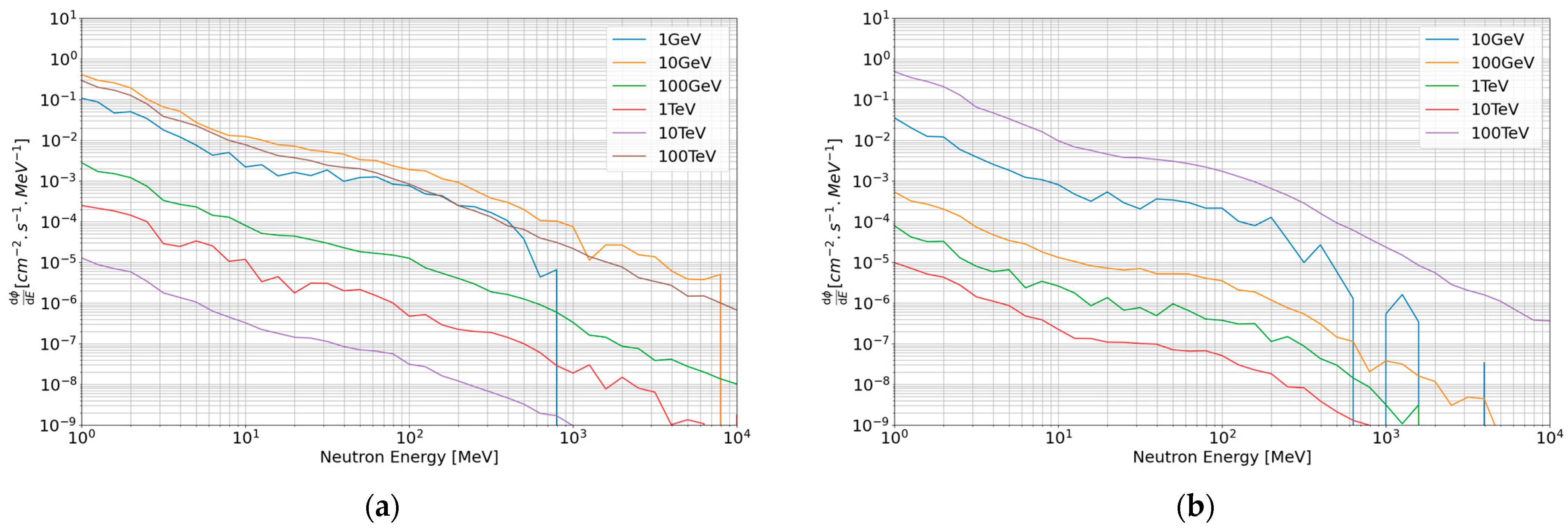
  • Then we convolute the average spectra to the population of primary particles at the position x and y at the time t with the energy E at 100 km, generating the convoluted spectra of the particle i created by the primary particle with the energy E at z altitude.
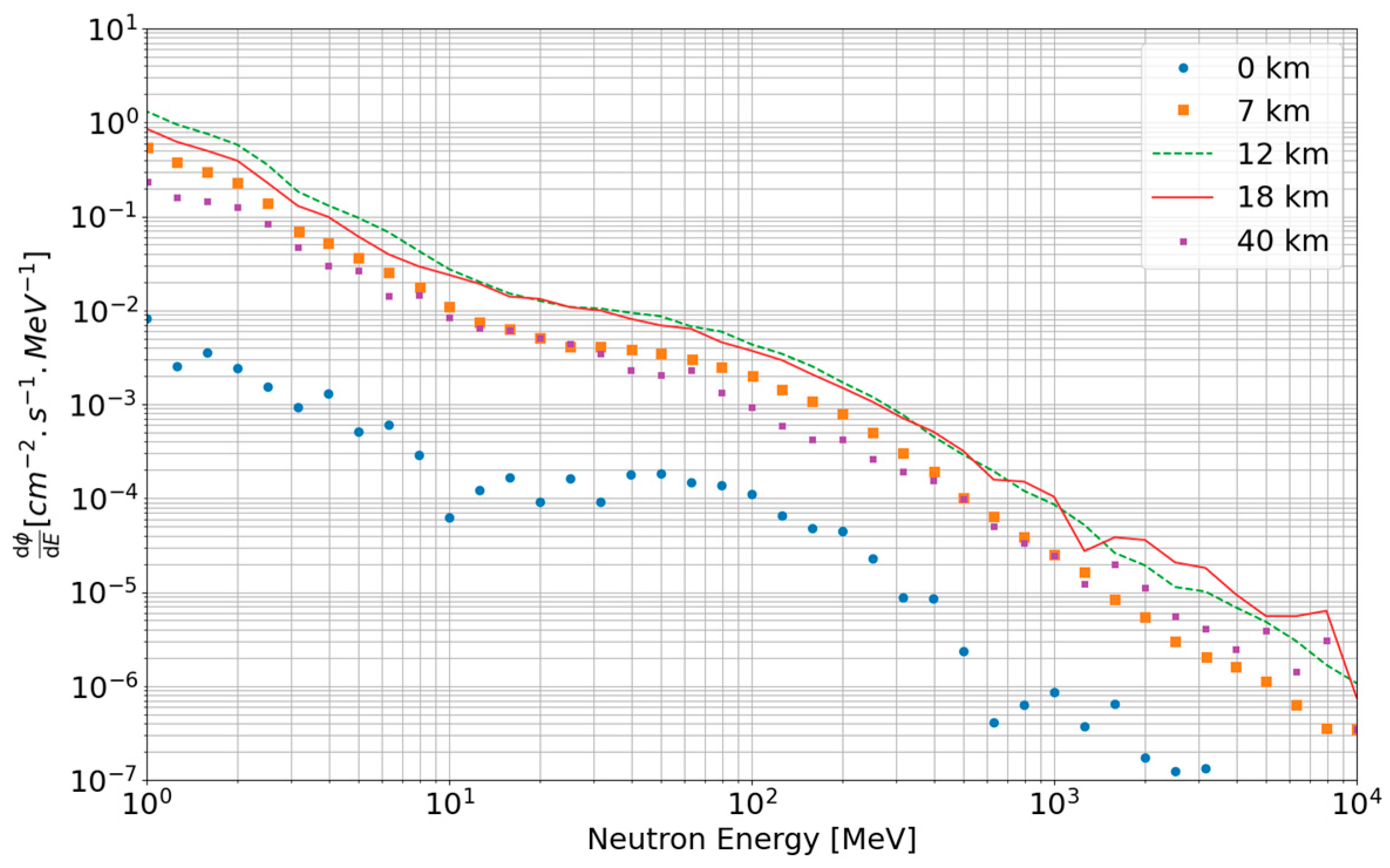
  • Finally, we compile all the convoluted spectra of the particle i at the altitude z , generating the spectra of particle i at the position x , y at the altitude z at the time t . To have an acceptable database size, we chose to focus on specific altitudes, which are z = 0 km, 3 km, 5 km, 7 km, 12 km, 18 km, and 40 km. This choice makes sense for ground level, avionic and stratospheric balloon applications.
In Figure 4, we present an example of the methodology to generate the spectra of neutrons at the position LAT, LON, at the time T and at the altitude Z.

3. Parameters Needed for the Simulations

There are two key parts to simulate EAS: the first one is the atmospheric modelling, and the second is the knowledge of primary particle flux coming from space. The definition of the atmosphere is primordial because the generation of the secondary particles starts with the nuclei of the atoms in the atmosphere. Moreover, the definition of the particles coming from outer space is also crucial, because they lead to the generation of the atmospheric radiative environment.

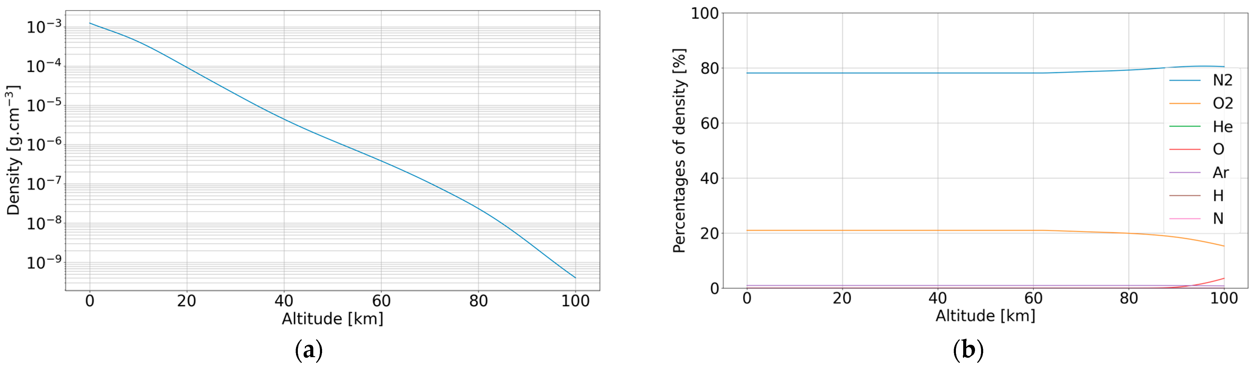
3.1. Constitution of the Atmosphere

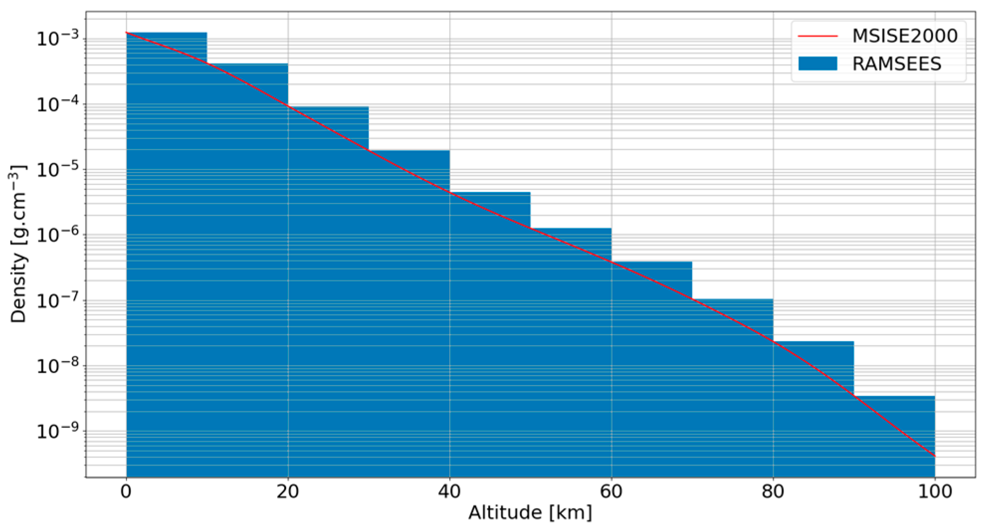
3.1.1. MSISE2000 Model

The NRLMSISE-00 [30] model is a model of the constitution of the atmosphere created by the NRL (Naval Research Laboratory). We selected the NRLMSISE-00 model using the Python version: nrlmsise00 [31] version 0.1.0 in this work. It allows the user to have, for a given location in the atmosphere at a given time, the constitution of the atmosphere. The main parameters are the total density of atoms, the density for a given gas and the temperature. In Figure 5, we show the result of MSISE200 for Paris France on 21 June of 2022. In Figure 5a, we plotted the evolution of the density of the atmosphere with altitude. Figure 5b shows the composition of the atmosphere as a function of altitude.
From Figure 5a,b, we can observe that the density decreases with the altitude, starting at 1.23 × 10 3 g . c m 3 at ground level and falling to 4.05 × 10 10 g . c m 3 at 100 km of altitude. In opposition to the evolution of the composition, the constitution is stable from 0 km to 60 km of altitude. The percentages of O2 and N2 are quite stable except at high altitudes (above 80 km), where we can observe some slight variations. We chose to model only O2 and N2 for the atmosphere because the third constituent (Argon) has an abundance lower than 1% whatever the altitude is.
Some variations occur between 60 km and 100 km of altitude but are compensated for by a very small global density at these altitudes, leading to few nuclear interactions. We decided to neglect them for the sake of simplicity.

3.1.2. Segmentations of the Atmosphere

Based on the results of the evolution of the atmosphere at a single location, we chose to discretize the atmosphere, in a first approximation, into ten blocks composed of 78.85% of N2 and 21.15% of O2, each with a height of 10 km. Each block has the density of the lowest altitude in the block. For example, in the 0 to 10 km block, the density is the one at 0 km.
In Figure 6, we plot the density of the atmosphere according to RAMSEES and to MSISE2000.

3.2. Primary Particles

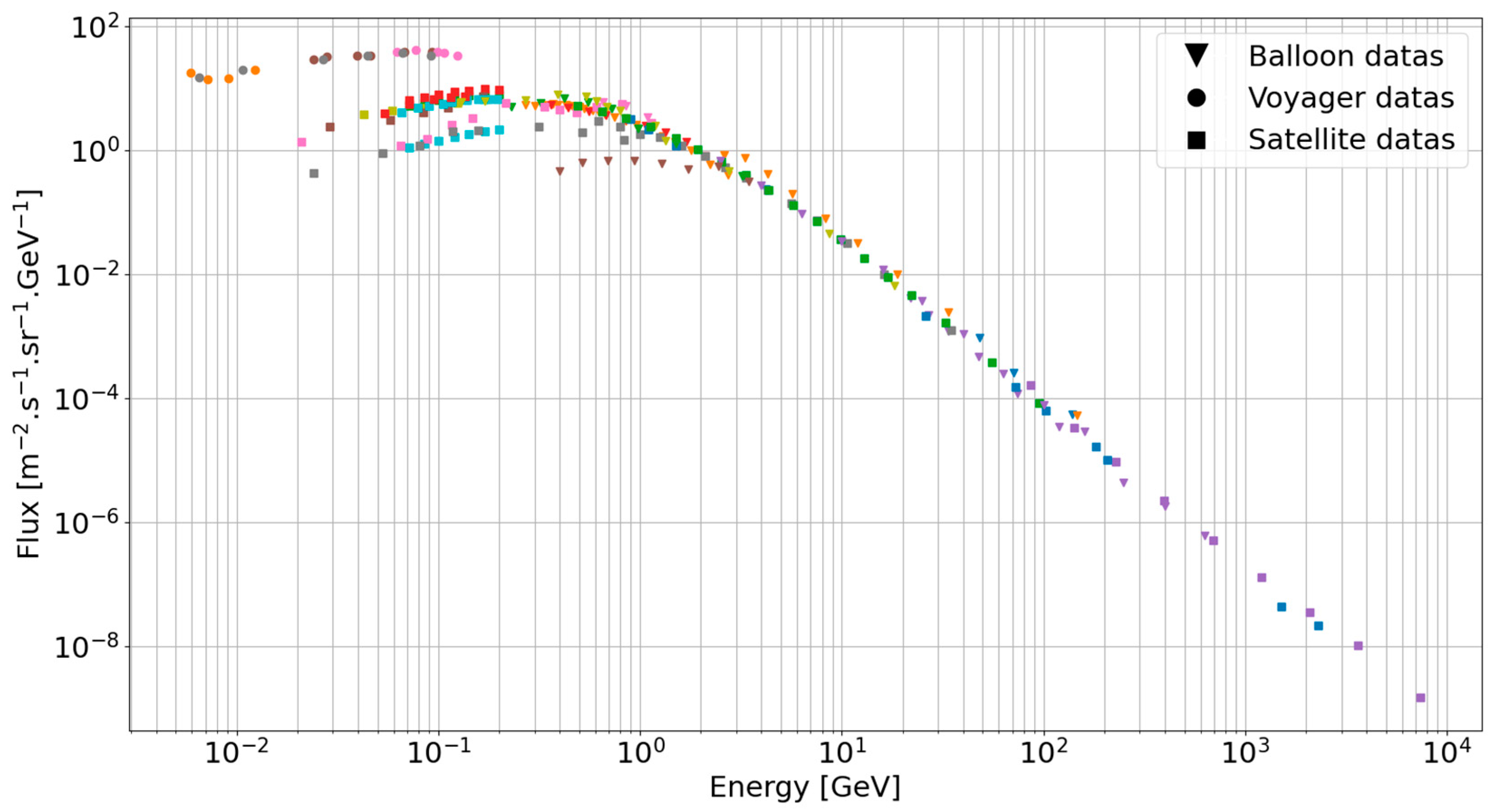
3.2.1. Compiling Proton Spectrum from Instrument and Model

The Cosmic Ray Data Base (CRDB) [32,33] compiles experimental data about cosmic rays measured in atmosphere with balloons, around the Earth from satellites and around the Solar System from Voyager 1 and 2. In the 4.0 version, the CRDB compiles the results of 116 experiments. Therefore, we chose it as the reference for our primary spectrum. Figure 7 presents a compilation of spectrum data from the CRDB. We observe a dispersion of the fluxes below 10 GeV because the lower energetic particles (<10 GeV) interact more with the heliosphere, the magnetosphere, the atmosphere and even the vehicle itself. Therefore, depending on the location (and the presence of an atmosphere or not) and the solar modulation [34,35], the particle flux obviously varies. Above 10 GeV, data are very similar whatever the measurement system, since the particles are too energetic to be affected enough to change the results.

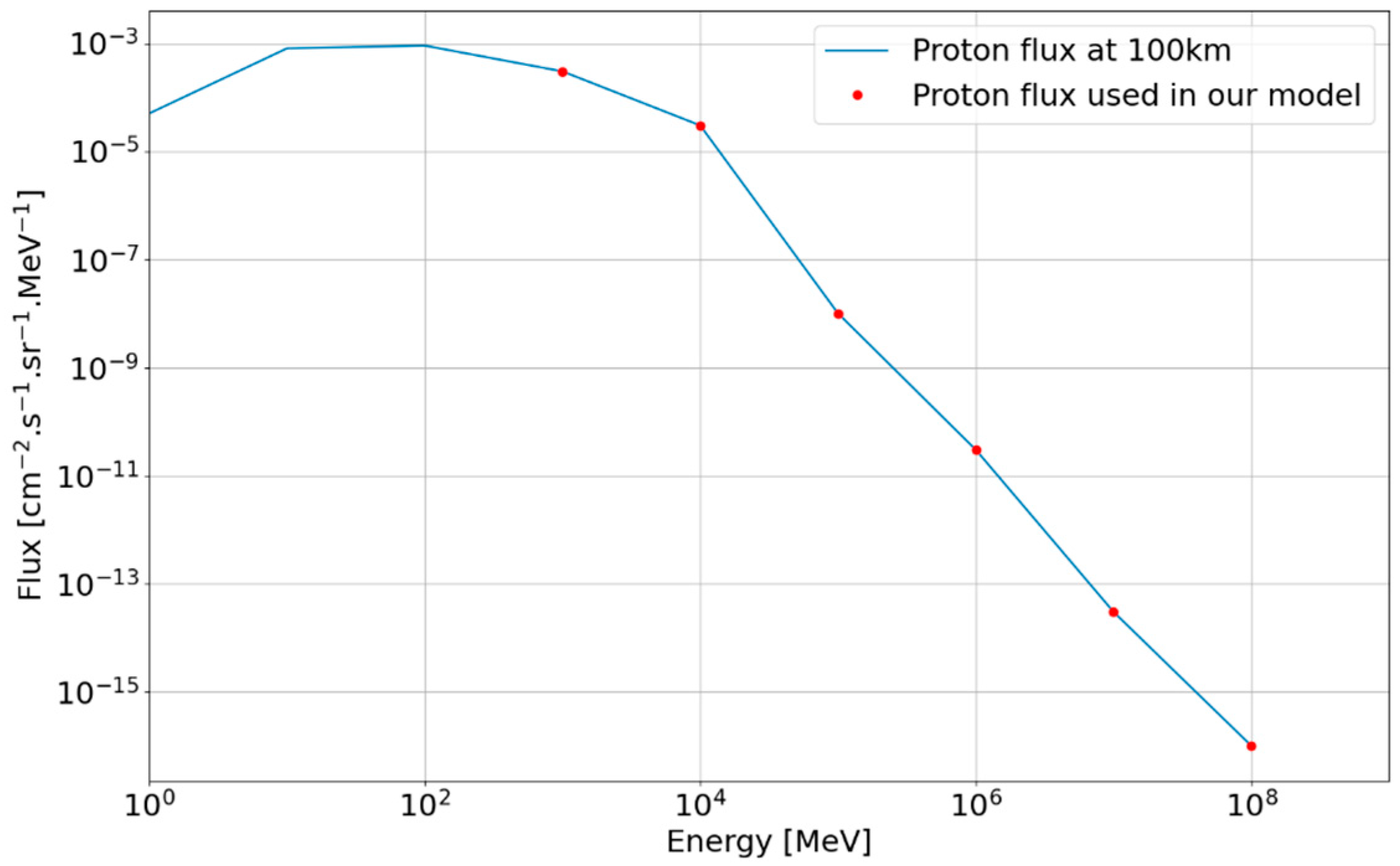
3.2.2. Discretization of the Primary Spectrum

In our approach, we simulate some monoenergetic protons to be able to reconstruct any primary spectrum. Because of the lack of accuracy of the data below 10 GeV, we focused our calculations above 1 GeV. We simulated proton primaries at energies of 1 GeV, 10 GeV, 100 GeV, 1 TeV, 10 TeV and 100 TeV. We simulated the particle of lowest energy of the bin, and we used it as a reference for the response of all the particles in the energy bin. This will allow the adding of new energies of a primary, reducing the bin size in the next version and so increasing the precision of RAMSEES with each version. In Figure 8, we present our primary spectrum of proton and the energies we choose to simulate. As an example of our methodology, in the energy bin 1 GeV to 10 GeV we simulated the 1 GeV proton EAS but integrated the population of the whole energy bin [1 GeV; 10 GeV] of the primary proton spectra. For the 1 GeV, 10 GeV and 100 GeV we simulated each primary proton energy for each single altitude 10 000 times, while for the 1 TeV, 10 TeV and 100 TeV we simulated each primary proton energy for each single altitude 300 times.
In Figure 9, we show the average calculation time for an extensive air shower in our simulation as a function of the incident energy. We observe that in a first approach, a power law can estimate the calculation time for one primary particle of a given energy: if we multiply the proton primary energy by 10, then we multiply the calculation time by 10. Based on this information, we chose to stop the primary spectrum at 100 TeV because of two parameters:
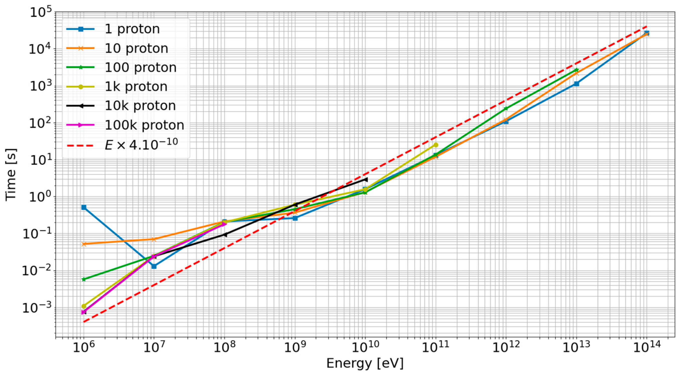
  • The calculation time: one proton of 100 TeV took, on average, 7 h to simulate on the CNES cluster, as shown in Figure 9. In total, we simulated for more than 300 million seconds equivalent 1 CPU (~10 years) in the CNES cluster.
  • The number of particles per time unit and surface, for a geometry of 30 km by 30 km at the top of the atmosphere: there is only one proton per second having an energy of 100 TeV or higher. This must be compared to the value of 13 × 10 15 of protons between 1 GeV and 10 GeV, which arrive on the same surface per second.
We did not make simulation below 1 GeV because our preliminary simulations showed that these particles could not create EAS big enough to reach below 30 km of altitude.

4. Monte Carlo Modelling and Extraction of the Model

4.1. Monte Carlo Simulation

To model the interaction of protons in the atmosphere, we chose the Geant4 toolkit version 10.6.0 [37,38]. Geant4 has many advantages. First, Geant4 is a well-known, robust, and used toolkit based on state-of-the-art physics developed by CERN and a coalition of scientists around the world. Secondly, Geant4 is a toolkit; therefore, it allows the user to be very flexible and to adapt the physics and the geometry to the problem. Thirdly, it is possible to use a pre-determined physics list in which all the recommended models are put together. In the Geant4 Physics list user manual [39], it is recommended to use QGSP_BERT [40] developed by Peter Speckmayer for High Energy Particles and secondary neutron production. It justifies the choice of QGSP_BERT as the physics list for our simulation.

4.2. Extracting Secondary Particle Spectrum from EAS Simulation

Compiling Simulation from the Same Energy

To be able to create a database of EAS transfer in the Earth atmosphere, we started by compiling all the results of our simulations by altitude and by particle, for a given energy of a primary proton. Then, we created an average response for each energy based on a Monte Carlo simulation, the Δ N i Δ E i z , with N i being the quantity of particles in the energy bin E i , the kind of secondary particle i at the given altitude z . As an example, we plotted in Figure 10 the spectrum for neutrons at 18 km of altitude. We can observe that the energy response is similar for each energy but that a more energetic primary creates more secondary neutrons. Moreover, higher energetic primaries create more secondaries, allowing better statistics to be obtained.
Applying Equation (1) to the primary spectrum of a given location and a given date, we computed the spectra of secondaries. In Figure 11a, we present the contribution of each part of the primary proton spectrum in the production of secondary neutrons at 18 km based on the primary particle population given in Figure 8. According to Figure 10, the number of secondary particles per primary proton increases with incident energy. However, because the flux of primary ions decreases with energy, we observe in Figure 11 that the primary proton energy that contributes the most to the secondary spectrum at 18 km is 10 GeV. In addition, the 100 TeV energy also contributes a lot to the neutron spectrum, not because of their abundance but because of their high energy, which allows triggering much more secondary particle generation. This is a crucial point, since it shows that we cannot neglect the contribution of very high-energy primary particles, which represent at least of 30% of the total spectrum. Moreover, the lower the altitude is, the higher the impact of the energy. In Figure 11b, we plotted the spectrum of secondary neutrons as a function of the energy of the incident proton at 7 km. In this case, we now observe a higher impact of the 100 TeV compared to 10 GeV, because the denser atmosphere has a greater impact on the lower-energy particles generated by the 10 GeV primary proton. The secondary particles generated by a 10 GeV have a lower energy than the ones from 100 TeV, and then are easily stopped by the atmosphere. The denser the atmosphere, the more energy the secondaries lose and the faster they stop. Finally, there is a very small contribution, less than 1%, of secondaries generated by the 1 GeV primary protons at 7 km.
Finally, by compiling all the energy responses, we get the spectrum plotted in Figure 12 for the secondary neutrons at 18 km and at 7 km based on the primary spectrum from Figure 8 (see Equation (1)).
In conclusion, by simulating monoenergetic proton entry at the top of the atmosphere, we developed a database of secondary particle spectra generated by EAS, designing RAMSEES to be adaptable to any primary particle spectra and making it compatible with every condition of space weather or cosmic ray model.
In parallel, we simulated energies higher by two orders of magnitude than any other model, because we observed that for ground applications it is necessary to simulate the highest energies (>1 TeV) of primary protons to correctly evaluate the spectrum of secondary particles involved in SEE.

5. Model Results and Analysis

In this part, we present RAMSEES results compared to experimental data and to the results given by the existing tools EXPACS and MAIRE. In Figure 13, we present RAMSEES results for neutrons at five altitudes: 0, 7, 12, 18 and 40 km. As expected, the neutron spectrum decreases rapidly with energy, in opposition to its evolution with the altitude where it increases from 40 km to 18 km and then decreases from 18 km to 0 km. There are two counterbalanced phenomena at play to explain this: (1) when the altitude decreases, the atmosphere density increases and the interaction is then more likely (and so the number of secondaries increases), and (2) because there are more and more interactions, the number of remaining primary particles decreases with decreasing altitude (and so the number of secondaries decreases). This combination of two counterbalanced effects leads to a maximum neutron flux at around 18 km. In first approximation, there are two orders of magnitude between ground level and avionic altitude (12 km).

5.1. Comparison with Experimental Data

To validate our results, we compared it to experimental data measured by several teams around the world.
In Figure 14, we compare RAMSEES results with the experimental data from two different instruments. The first set of data was collected at Pic du Midi, France (2.9 km of altitude) from May 2011 to 2018 with a Bonner Sphere System (BSS) neutron spectrometer and the second one at Plateau de Rosa, Italy (3.5 km of altitude) in January 1998 with a Bubble Detector Spectrometer, a passive system, by Hubert et al. [41]. The Pic du Midi experiment collected data for 8 years. When comparing our predictions at 3 km and the in-situ data at Pic du Midi, we need to consider that there is a difference of 100 m of altitude between them. Despite the 100 m of altitude difference, RAMSEES shows a good agreement with the data from Pic du Midi with less than a factor 1.55 of difference. In the case of Plateau Rosa, we observe a factor 2.38 of difference between RAMSEES model and the experimental data below 1 GeV. However, there are two main factors to consider here. First, the data were acquired during one month at a solar minimum, implying a maximum of atmospheric radiation, and secondly, the 500 m of altitude of difference influences the spectrum, making it higher in the case of Plateau the Rosa than at 3 km. At higher energies than 1 GeV, we observe a divergence between our prediction and the in-situ measurements. We think the divergence is caused by the solar minimum allowing more cosmic rays to enter the Solar System and the Earth’s atmosphere. All together, we can say that the RAMSEES model fits with the experimental data at 2.9 km but shows discrepancies at 3.5 km. The comparison of a worst-case scenario (solar minimum) to the 3.5 km data should be interesting to do to extend the validation of RAMSEES.

5.2. Comparison to Existing Models

In the following, we compare the RAMSEES model to the standards, which are the JEDEC and the IEC, and also to existing tools, namely EXPACS and MAIRE. The JEDEC standard gives a neutron flux at New York, United States of America at Sea Level and the IEC standard gives an analytical formula to extract the neutron spectrum at 12 km of altitude.
In Figure 15a, we compare the JEDEC to EXPACS, MAIRE and RAMSEES at ground level. We observe that between 1 MeV and 10 GeV there is a maximum of a factor of 10 between RAMSEES, EXPACS, MAIRE and the JEDEC. RAMSEES has a very good agreement with the JEDEC up to 40 MeV and, like MAIRE, RAMSEES overestimates the number of neutrons from 40 MeV to 400 MeV. In the same way, we compare, in Figure 15b, the IEC to EXPACS, MAIRE and RAMSEES at 12 km. We observe a very good agreement between RAMSEES and the IEC from 3 MeV to 3000 MeV with less than a factor of 2. RAMSEES agrees with MAIRE above 10 MeV but not below 10 MeV, where RAMSEES gives a flux 2 times higher than MAIRE. However, RAMSEES disagrees with EXPACS on the whole spectrum by a factor of 6, which will be discussed later.
In Figure 16a,b, we compare the results of RAMSEES with EXPACS and MAIRE at 7 and 18 km, respectively. We observe that, at 7 km and 18 km, the spectra generated by RAMSEES and by EXPACS are, again, separated by a factor of 6. This is in opposition to the observation between results from MAIRE and RAMSEES, for which the difference is less than a factor of 2, except below 10 MeV, where RAMSEES tends to predict higher fluxes than MAIRE. At 18 km, we observe that RAMSEES and MAIRE give the same results from 400 keV to 5 GeV, except for two differences: the first one at 500 MeV, which is a difference of a factor of 2; and the second one at 1.1 GeV, by a factor of 5. We think these two differences can be explained by statistical issues on our side, because the values before and after these energies are equivalent to MAIRE values in the two cases.

6. Conclusions and Discussions

In this paper, we presented our model RAMSEES (Radiation Atmospheric Model for SEE Simulation), which is a database, built by Monte-Carlo simulation, composed of the response of the atmosphere to cosmic rays. We modeled the atmosphere with the results given by the NRLMSISE-00 model and used the CRDB and the Swordy plot as reference for the primary protons coming from space. Then, we simulated the Extensive Air Shower (EAS) phenomenon by making Monte Carlo simulations of the interactions of monoenergetic proton via the Geant4 toolkit with the QGSP_BERT physics list. We stopped our simulation at 100 TeV per proton because there is only one proton per geometry per second and because of the very high computational time required at high energy. Finally, we compiled the results of the monoenergetic primary simulation with the spectrum of protons coming from space, creating for each altitude a spectrum of neutrons and of protons.
In opposition to MAIRE and EXPACS, which were built to calculate dose rates for flight crews, RAMSEES was built to allow the SEE rate calculations from ground level to space. By using a physics list dedicated to high-energy particles and to neutron generation, we created a model designed to estimate electronic failures induced by neutrons and protons from ground level to 100 km. Moreover, we showed in this work that the higher energetic part of the primary spectrum is primordial for calculating the secondary spectrum below 18 km. That is why we simulated two more orders of magnitude in the energy of primary particles than in any other models, to make RAMSEES reliable down to ground level.
RAMSEES could be used for the airplane industry, scientific balloons and even the automotive industry, to estimate the SEE rates in their electronic devices. Moreover, RAMSSES allows the user to know the flux of neutron and proton at any given location, and any time, making it compatible with any cosmic ray model.
Our model provides very encouraging results when compared with existing experimental results, other models, and standards:
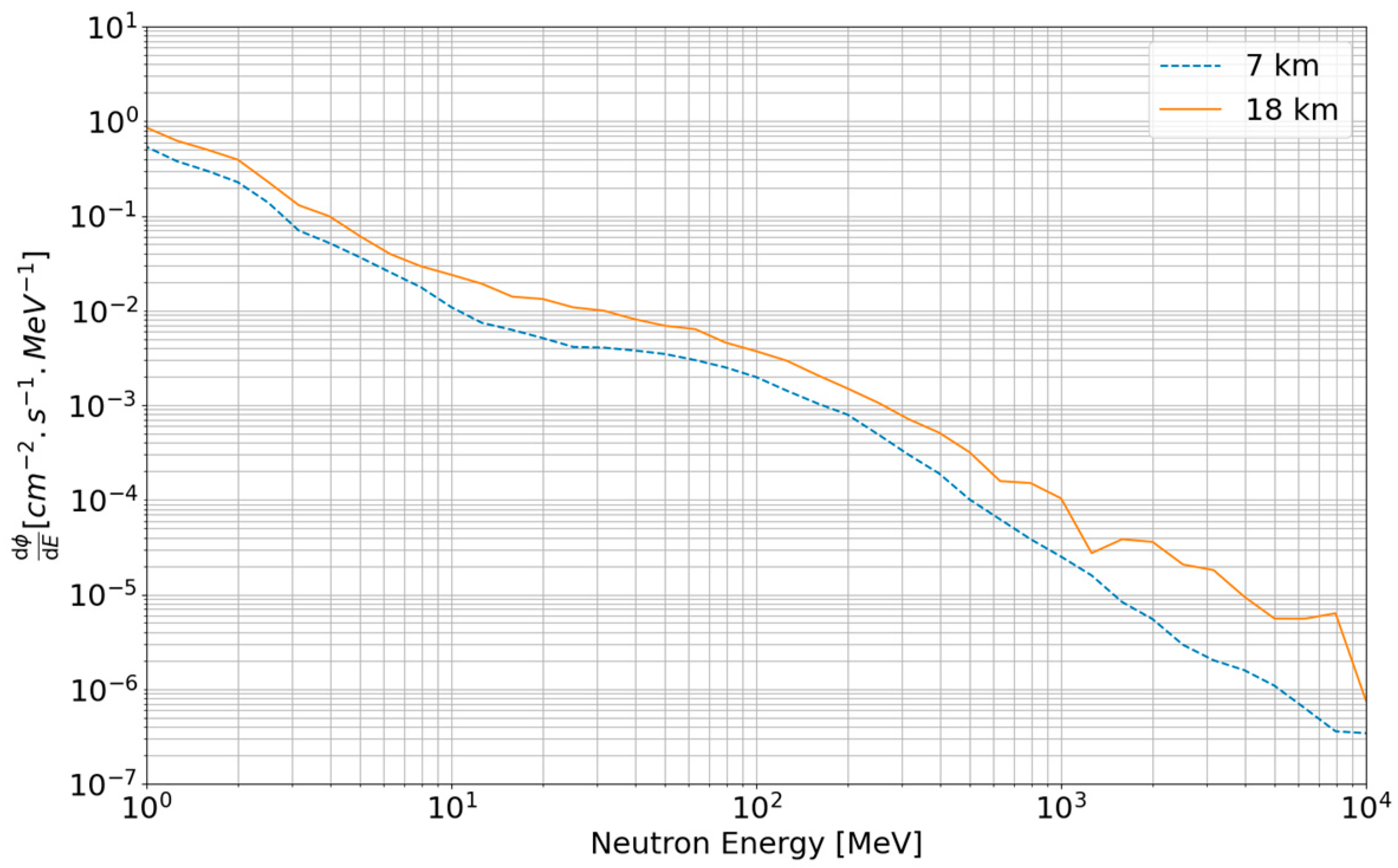
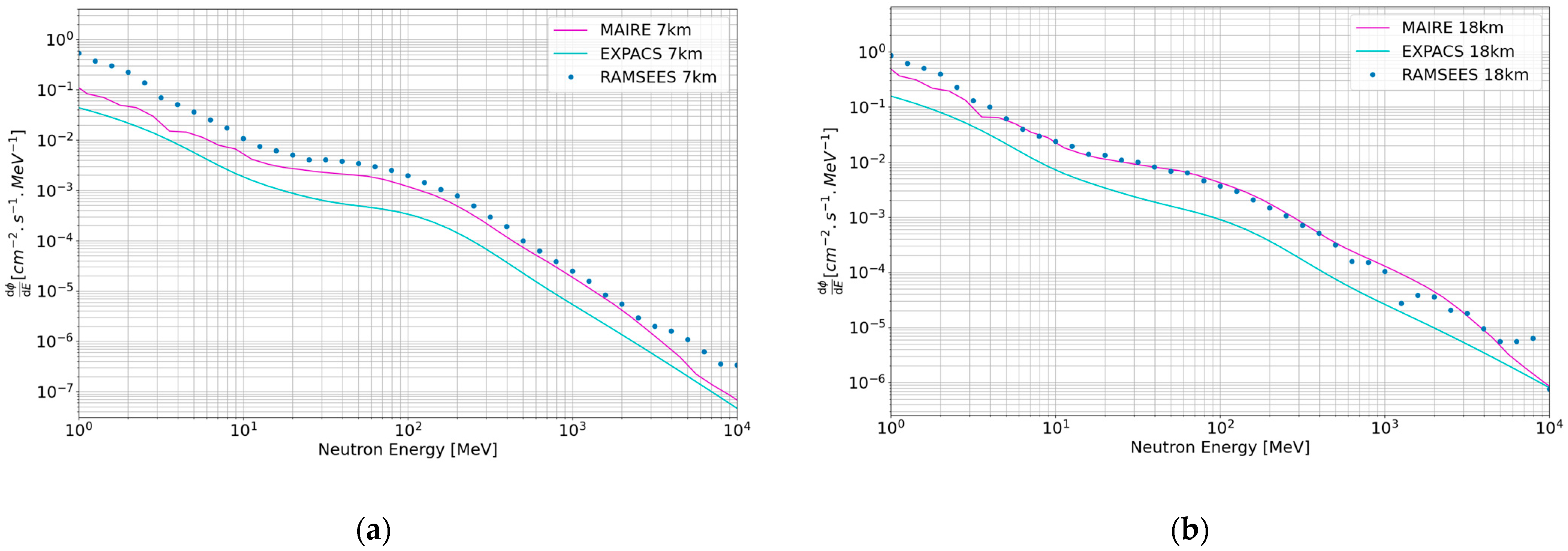
  • At high altitude (18 km), our results are in very good agreement with MAIRE.
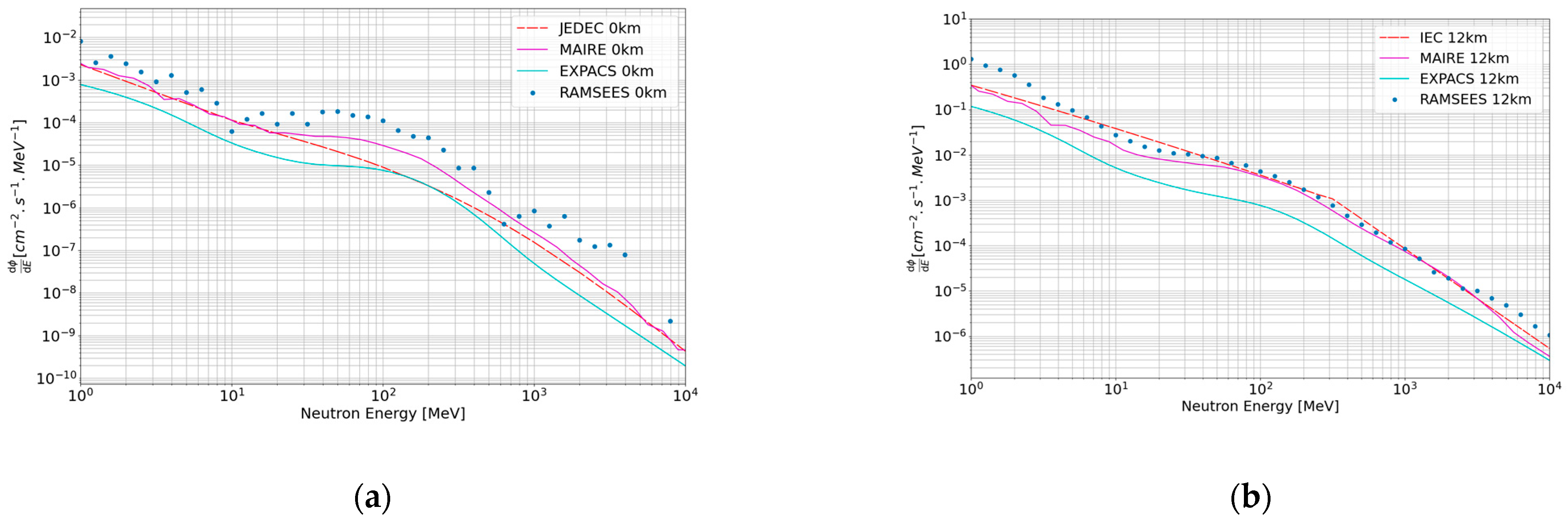
  • At avionic altitude (12 km), our results are in good agreement with both MAIRE and IEC standard. RAMSEES seems to overestimate neutron flux below 10 MeV, which is not an issue since electronic devices are not sensitive to fast neutrons below a few MeV.
  • At 7 km of altitude, we have the same trend as MAIRE but with a slight enhancement of neutron flux. We cannot claim which one is closer to the real flux, and more experimental data are required. Regarding concerns over electronic reliability, it is probably better to overestimate the risk.
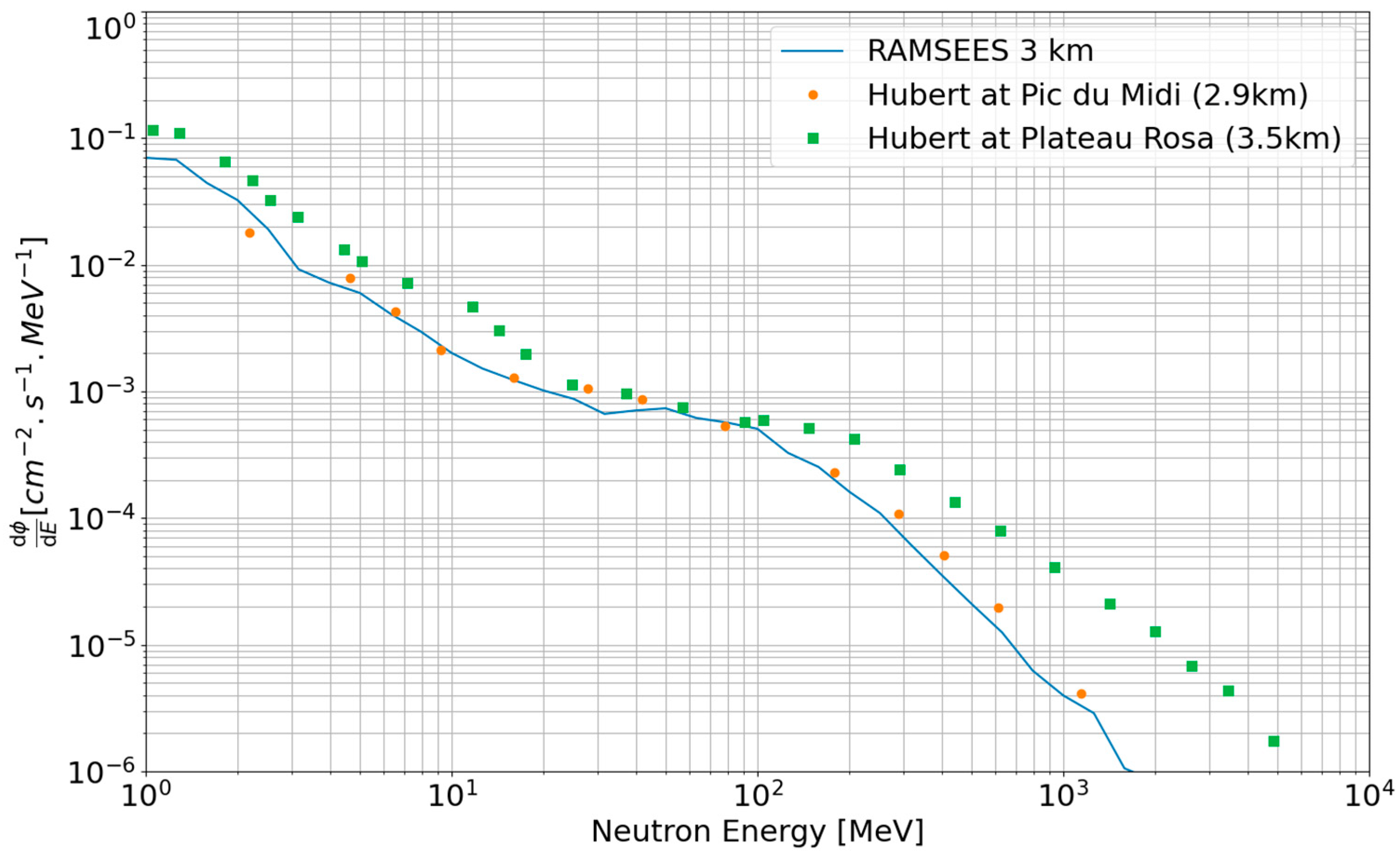
  • At 3 km of altitude, RAMSEES shows a good agreement with experimental data at 3 km, if we compare them to 8 years of experimental data at Pic du Midi at 2.9 km.
  • At ground level, our results have a shape similar to those of MAIRE and JEDEC spectra. However, here again, we seem to overestimate the risk, compared to the other models.
As far as EXPACS is concerned, we observed a factor of 6 between this work and the flux given by EXPACS at any altitude. We suppose that it may be due to a missing factor of 2π in EXPACS that should account for all particle directions; however, we cannot be sure of this, as we do not have details of the calculations. Finally, to be able to compare the three models with more precision and to understand the differences, it would be necessary to have access to the precise methodology and equations used by the other two models. However, this information is currently not available, for proprietary reasons.
This work is an attempt to model the radiation environment in the atmosphere. It is encouraging even if not perfect, and some points could be improved in the future. Among these are:
  • The physics list of Geant4 is not the best when dealing with such high energies. Alternately, it could be possible to link Geant4 with CRMC [42,43].
  • The discretization of the atmosphere into layers could be improved by increasing the number of layers.
  • The number of primary proton energies used for the simulation could be increased.
  • Some more comparisons are also possible with other existing tools such as MCeq [44].
To conclude, the results of this work fill the need for CNES scientific balloon applications as well as for avionic industry applications, which experience reliability issues due to natural radiation. RAMSEES will allow evaluating the flux of neutrons and protons needed to calculate failure rates at ground level, avionic altitude, or stratospheric altitude, making them able to design their electronic devices to better resist the atmospheric radiative environment. To do so, we will need to link RAMSEES to a prediction tool able to transport neutrons in electronic devices, to simulate nuclear reactions induced by neutrons in the silicon of the chip, and to determine whether a single event effect occurs or not.

Author Contributions

Conceptualization, H.C., F.W. and M.R.; methodology, H.C., F.W., F.S. and D.H.; software, H.C.; validation, H.C.; writing—original draft preparation, H.C., F.W. and F.S.; writing—review and editing, F.W., F.S., D.H., M.R., F.B. and J.M.; supervision, F.W., F.S., F.B. and A.V.; funding acquisition, F.W., F.B., J.M. and A.V. All authors have read and agreed to the published version of the manuscript.

Funding

This work was co-funded by the French Government through the CNES, the French Space Agency and by the TRAD company.

Data Availability Statement

Data presented in this study are not available for sharing due to proprietary issue.

Conflicts of Interest

The authors declare no conflict of interest.

References

  1. Van Allen, J.A.; McIlwain, C.E.; Ludwig, G.H. Radiation observations with satellite 1958 ε. J. Geophys. Res. 1959, 64, 271–286. [Google Scholar] [CrossRef]
  2. Auger, P.; Ehrenfest, P.; Maze, R.; Daudin, J.; Fréon, R.A. Extensive Cosmic-Ray Showers. Rev. Mod. Phys. 1939, 11, 288–291. [Google Scholar] [CrossRef]
  3. Rossi, B. On the Magnetic Deflection of Cosmic Rays. Phys. Rev. 1930, 36, 606. [Google Scholar] [CrossRef]
  4. Rao, M.V.S.; Sreekantan, B.V. Extensive Air Showers; World Scientific: Singapore, 1998. [Google Scholar]
  5. Clem, J.M.; De Angelis, G.; Goldhagen, P.; Wilson, J. New calculations of the atmospheric cosmic radiation field—results for neutron spectra. Radiat. Prot. Dosim. 2004, 110, 423–428. [Google Scholar] [CrossRef]
  6. Liu, H.; Hou, Y.; Li, H.; Song, Y.; Hu, L.; Liang, M. Cosmic-ray neutron fluxes and spectra at different altitudes based on Monte Carlo simulations. Appl. Radiat. Isot. 2021, 175, 109800. [Google Scholar] [CrossRef]
  7. Pazianotto, M.T.; Cortés-Giraldo, M.A.; Federico, C.A.; Gonçalez, O.L.; Quesada, J.M.; Carlson, B.V. Determination of the cosmic-ray-induced neutron flux and ambient dose equivalent at flight altitude. J. Phys. Conf. Ser. 2014, 630, 012022. [Google Scholar] [CrossRef] [Green Version]
  8. Pastircak, B.; Bobik, P.; Putiš, M.; Bertaina, M.; Fenu, F.; Shinozaki, K.; Szabelski, J.; Santangelo, A. Modelling Muon and Neutron Fluxes and Spectra on the Earth’s Ground Induced by Primary Cosmic Rays. In Proceedings of the 34th International Cosmic Ray Conference (ICRC2015), The Hague, The Netherlands, 30 July–6 August 2015. [Google Scholar] [CrossRef] [Green Version]
  9. Overholt, A.C.; Melott, A.L.; Atri, D. Modeling cosmic ray proton induced terrestrial neutron flux: A look-up table. J. Geophys. Res. Space Phys. 2013, 118, 2765–2770. [Google Scholar] [CrossRef] [Green Version]
  10. Taber, A.; Normand, E. Single event upset in avionic. IEEE Trans. Nucl. Sci. 1993, 40, 120–126. [Google Scholar] [CrossRef]
  11. Normand, E. Single Event Effects in Avionics. IEEE Trans. Nucl. Sci. 1996, 43, 461–474. [Google Scholar] [CrossRef]
  12. JEDEC. Measurement and Reporting of Alpha Particle and Terrestrial Cosmic Ray Induced Soft Error in Semiconductor Devices; JEDEC: Arlington, VA, USA, 2021. [Google Scholar]
  13. IEC 62396-1:2016; Process Management for Avionics—Atmospheric Radiation Effects—Part 1: Accommodation of Atmospheric Radiation Effects Via Single Event Effects within Avionics Electronic Equipment. International Electrotechnical Commission: Geneva, Switzerland, 2016.
  14. MAIRE+ Demonstration Website. Surrey Space Centre. Available online: https://spaceweather.surrey.ac.uk/ (accessed on 12 December 2022).
  15. EXPACS Homepage. JAEA. Available online: https://phits.jaea.go.jp/expacs/ (accessed on 12 December 2022).
  16. Ziegler, J. Terrestrial cosmic rays. IBM J. Res. Dev. 1996, 40, 19–39. [Google Scholar] [CrossRef]
  17. Models for Atmospheric Ionising Radiation Effects—MAIRE. Available online: http://maire.uk (accessed on 15 January 2023).
  18. Lei, F.; Clucas, S.; Dyer, C.; Truscott, P. An atmospheric radiation model based on response matrices generated by detailed Monte Carlo Simulations of cosmic ray interactions. IEEE Trans. Nucl. Sci. 2004, 51, 3442–3451. [Google Scholar] [CrossRef]
  19. Lei, F.; Hands, A.; Clucas, S.; Dyer, C.; Truscott, P. Improvement to and Validations of the QinetiQ Atmospheric Radiation Model (QARM). IEEE Trans. Nucl. Sci. 2006, 53, 1851–1858. [Google Scholar] [CrossRef]
  20. Hands, A.; Lei, F.; Davis, C.; Clewer, B.; Dyer, C.; Ryden, K. A New Model for Nowcasting the Aviation Radiation Environment with Comparisons to In Situ Measurements Durign GLEs. Space Weather 2022, 20, e2022SW003155. [Google Scholar] [CrossRef]
  21. Sato, T.; Niita, K. Analytical functions to predict cosmic-ray neutron spectra in the atmosphere. Radiat. Res. 2006, 166, 544–555. [Google Scholar] [CrossRef]
  22. Sato, T.; Yasuda, H.; Niita, K.; Endo, A.; Shiver, L. Development of PARMA: PHITS based Analytical Radiation Model in the Atmosphere. Radiat. Res. 2008, 170, 244–259. [Google Scholar] [CrossRef]
  23. Sato, T. Analytical Model for Estimating Terrestrial Cosmic Ray Fluxes Nearly Anytime and Anywhere in the World: Extension of PARMA/EXPACS. PLoS ONE 2015, 10, e0144679. [Google Scholar] [CrossRef] [Green Version]
  24. Sato, T. Analytical Model for Estimating the Zenith Angle Dependence of Terrestrial Cosmic Ray Fluxes. PLoS ONE 2016, 11, e0160390. [Google Scholar] [CrossRef] [Green Version]
  25. Sato, T.; Niita, K.; Matsuda, N.; Hashimoto, S.; Iwamoto, Y.; Noda, S.; Ogawa, T.; Iwase, H.; Nakashima, H.; Fukahori, T.; et al. Particle and Heavy Ion Transport code System, PHITS, version 2.52. J. Nucl. Sci. Technol. 2013, 50, 913–923. [Google Scholar] [CrossRef] [Green Version]
  26. Hubert, G.; Bezerra, F.; Nicot, J.-M.; Artola, L.; Cheminet, A.; Valdivia, J.-N.; Mouret, J.-M.; Meyer, J.-R.; Cocquerez, P. Atmospheric Radiation Environment Effects on Electronic Balloon Board Observed During Polar Vortex and Equatorial Operational Campaigns. IEEE Trans. Nucl. Sci. 2014, 61, 1703–1709. [Google Scholar] [CrossRef]
  27. Agostinelli, S.; Allison, J.; Amako, K.A.; Apostolakis, J.; Araujo, H.; Arce, P.; Asai, M.; Axen, D.; Banerjee, S.; Barrand, G.; et al. Geant4—A simulation toolkit. Nucl. Instrum. Methods Phys. Res. Sect. A Accel. Spectrometers Detect. Assoc. Equip. 2003, 506, 250–303. [Google Scholar] [CrossRef] [Green Version]
  28. Allison, J.; Amako, K.; Apostolakis, J.; Araujo, H.; Arce Dubois, P.; Asai, M.; Barrand, G.; Capra, R.; Chauvie, S.; Chytracek, R.; et al. Geant4 Developments and Applications. IEEE Trans. Nucl. Sci. 2006, 53, 270–278. [Google Scholar] [CrossRef] [Green Version]
  29. Allison, J.; Amako, K.; Apostolakis, J.; Arce, P.; Asai, M.; Aso, T.; Bagli, E.; Bagulya, A.; Banerjee, S.; Barrand, G.; et al. Recent developments in Geant4. Nucl. Instrum. Methods Phys. Res. Sect. A Accel. Spectrometers Detect. Assoc. Equip. 2016, 835, 186–225. [Google Scholar] [CrossRef]
  30. Picone, J.M.; Hedin, A.; Drob, D.; Aikin, A.C. NRLMSISE-00 empirical model of the atmosphere: Statistical comparisons and scientific issues. J. Geophys. Res. 2002, 107, 1468. [Google Scholar] [CrossRef]
  31. nrlmsise00. Available online: https://pypi.org/project/nrlmsise00/ (accessed on 6 October 2021).
  32. Maurin, D.; Melot, F.; Taillet, R. A database of charged cosmic rays. Astron. Astrophys. 2014, 569, A32. [Google Scholar] [CrossRef] [Green Version]
  33. Maurin, D.; Dembinski, H.; Gonzalez, D.; Maris, L.; Frédéric, M. Cosmic-Ray Database Update: Ultra-High Energy, Ultra-Heavy, and Antinuclei Cosmic-Ray Data (CRDB v4.0). Universe 2020, 6, 102. [Google Scholar] [CrossRef]
  34. Terashima, Y. Solar Modulation of Primary Cosmic Rays. Prog. Theor. Phys. 1960, 23, 1138–1150. [Google Scholar] [CrossRef] [Green Version]
  35. Potgieter, M.S. Solar Modulation of Cosmic Rays. Living Rev. Sol. Phys. 2013, 10, 3. [Google Scholar] [CrossRef] [Green Version]
  36. Hanlon, W. Cosmic Ray Spectra of Various Instruments. Available online: https://web.physics.utah.edu/~whanlon/spectrum.html (accessed on 4 January 2023).
  37. Software Download Archive—Geant4 10.6. Geant4, 6 December 2019. Available online: https://geant4.web.cern.ch/support/download_archive?page=1 (accessed on 6 December 2022).
  38. GitHub Geant4 Release v10.6.0. Geant4, 6 December 2019. Available online: https://github.com/Geant4/geant4/releases/tag/v10.6.0 (accessed on 6 December 2022).
  39. Physics Reference Manual Release 11.0. Available online: https://geant4-userdoc.web.cern.ch/UsersGuides/PhysicsReferenceManual/fo/PhysicsReferenceManual.pdf (accessed on 28 November 2022).
  40. Apostolakis, J.; Folger, G.; Grichine, V.; Heikkinen, A.; Howard, A.; Ivanchenko, V.; Kaitaniemi, P.; Koi, T.; Kosov, M.; Quesada, J.M.; et al. Progress in hadronic physics modelling in Geant4. J. Phys. Conf. Ser. 2009, 160, 012073. [Google Scholar] [CrossRef]
  41. Hubert, G.; Silvia, V.; Alba, Z. Temporal Series Analyses of Cosmic-Ray-Induced-Neutron Spectra Measured in High-Altitude During the Last Two Decades. In Proceedings of the 36th International Cosmic Ray Conference (ICRC 2019), Madison, WI, USA, 24 July–1 August 2019. [Google Scholar]
  42. Available online: https://web.ikp.kit.edu/rulrich/crmc.html (accessed on 15 January 2023).
  43. Andrii, T.; David, D.; Chuan, Y.; Mingyang, C.; Xiang, L.; Xin, W. TeV–PeV Hadronic Simulations with DAMPE. In Proceedings of the 36th International Cosmic Ray Conference (ICRC 2019), Madison, WI, USA, 24 July–1 August 2019; p. 143. [Google Scholar] [CrossRef]
  44. Available online: https://pypi.org/project/MCEq/ (accessed on 15 January 2023).
Figure 1. Schematic of the Extensive Atmospheric Shower phenomenon (proton: red, electron: green, photon: yellow, neutron: blue, muon: purple).
Aerospace 10 00295 g001
Figure 2. Approach and components needed to simulate an EAS.
Aerospace 10 00295 g002
Figure 3. Schematic of the atmosphere and its projection in our Monte Carlo simulation.
Aerospace 10 00295 g003
Figure 4. Schematic of the extraction of spectra at an altitude Z from the file of simulated data on the cluster to the user spectra of neutron based on the primary spectra at LAT, LON at the time T.
Aerospace 10 00295 g004
Figure 5. Evolution of the atmospheric composition and density based on MSISE2000 for Paris, France on 21 June 2022: (a) Evolution of the atmosphere density as a function of altitude; (b) Evolution of the constitution of the atmosphere as a function of altitude.
Aerospace 10 00295 g005
Figure 6. Density of the atmosphere in this work compared to MSISE2000.
Aerospace 10 00295 g006
Figure 7. Proton spectrum based on data from several instruments on Voyager, satellite or balloon extracted from the CRDB. Each color is a different experiment.
Aerospace 10 00295 g007
Figure 8. Discretization of the proton spectrum at 100 km of altitude based on the Swordy plot by William Hanlon [36] and the CRDB.
Aerospace 10 00295 g008
Figure 9. Average time of calculation of one primary particle Extensive Air Shower according to its energy and the number of primary particles simulated.
Aerospace 10 00295 g009
Figure 10. Spectrum of secondary neutrons for one incident proton at 18 km of altitude.
Aerospace 10 00295 g010
Figure 11. Spectrum of secondary neutrons according to the energy of the incident proton generated by each part of the primary particles spectrum given in Figure 8 at two altitudes: (a) at 18 km and (b) at 7 km.
Aerospace 10 00295 g011
Figure 12. Spectrum of secondary neutrons at 7 and 18 km given by RAMSEES (Radiation Atmospheric Model for Single Event Effect Simulation).
Aerospace 10 00295 g012
Figure 13. Flux of neutrons given by RAMSEES at different altitudes.
Aerospace 10 00295 g013
Figure 14. Comparison between RAMSEES results at 3 km and experimental data at 2.9 and 3.5 km from Hubert et al. [40].
Aerospace 10 00295 g014
Figure 15. RAMSEES spectrum of secondary neutrons at several altitudes compared to standard and to the models MAIRE & EXPACS: (a) ground level compared to JEDEC; (b) 12 km of altitude compared to IEC.
Aerospace 10 00295 g015
Figure 16. Spectrum of secondary neutrons compared to EXPACS and MAIRE at several altitudes: (a) at 7 km and (b) at 18 km.
Aerospace 10 00295 g016
Disclaimer/Publisher’s Note: The statements, opinions and data contained in all publications are solely those of the individual author(s) and contributor(s) and not of MDPI and/or the editor(s). MDPI and/or the editor(s) disclaim responsibility for any injury to people or property resulting from any ideas, methods, instructions or products referred to in the content.

