Article

Propagation of Interactions among Aircraft Trajectories: A Complex Network Approach

by
Raúl López-Martín
and
Massimiliano Zanin
*
Instituto de Física Interdisciplinar y Sistemas Complejos CSIC-UIB, Campus Universitat de les Illes Balears, E-07122 Palma de Mallorca, Spain
*
Author to whom correspondence should be addressed.
Aerospace 2023, 10(3), 213; https://doi.org/10.3390/aerospace10030213
Submission received: 30 November 2022 / Revised: 27 January 2023 / Accepted: 21 February 2023 / Published: 24 February 2023
(This article belongs to the Section Air Traffic and Transportation)

Abstract

:
Interactions between aircraft, as, e.g., those caused by minimum separation infringements, can trigger non-local cascades of interactions that can propagate over large temporal and spatial scales. Assessing those downstream effects is a computationally complex problem, which has only been tackled over rather limited time horizons. We here propose a methodology to map these interactions into networks, thus representing their potential propagation and the structure induced by them. The result is a conceptually simple and computationally tractable representation, which can be further analyzed using metrics provided by a complex networks theory. We firstly test this methodology using a synthetic airspace, then move on to the analysis of planned and executed trajectories for a large European airspace in the year 2018. We show how these propagation networks reflect the structure of airways, the intervention of air traffic controllers, and how they have evolved through time. We finally discuss potential real-world applications, and some key aspects that need to be further studied to make this a viable instrument in an operational context.

1. Introduction

One of the most important missions of air traffic control is to ensure the safety of flights inside an airspace, and specifically that minimum separation distances are maintained to prevent mid-air collisions [1]—instances of minimum separation infringements are called “conflicts”. This was initially achieved by a combination of three elements: a fixed route network, forcing aircraft to follow predefined paths; the intervention of air traffic controllers; and the use of last-ditch systems for detecting and resolving conflicts, such as the Traffic alert and Collision Avoidance System (TCAS). Under low traffic volumes, the task of preventing conflicts is a simple one, usually only requiring changing the trajectory of one (or of both) of the aircraft involved in the event. This nevertheless became more complex in the last few decades. On one hand, fixed route networks come with the drawback of a reduction in efficiency, and operational concepts not relying on them (such as, e.g., free routing) are being implemented; yet, these imply an increase in the heterogeneity of traffic interactions [2]. On the other hand, the increasing air traffic demand and the consequent increase in flight density imply that conflicts can involve more than two aircraft at the same time; and the presence of situations in which the resolution of one conflict may create a new one, i.e., the presence of downstream effects [3].
Manually predicting the downstream consequences of a change in the trajectory of one or more aircraft is a challenging task for air traffic controllers, and even existing automatic conflict detection and resolution systems are known to be able to analyze only short-term horizons [4]. To illustrate such complexity, let us consider the case of a set of aircraft following previously deconflicted trajectories—in other words, if they were to exactly follow the flight plans, no conflict would arise. Let us further suppose that one of them has its trajectory modified, e.g., due to some local winds, and that this generates a conflict with a second aircraft. Such a safety event would be solved by the air traffic controller by changing the former aircraft’s trajectory, resulting in that aircraft recovering the originally planned route at a different time (either before, or more frequently, after what was planned). This also implies that the aircraft may end up in additional conflicts, as its trajectory does not correspond anymore with the initially planned and deconflicted one. Most importantly, these subsequent conflicts can happen at any point of the flight, i.e., even after long periods of time; and can further trigger a cascade, in which one conflict forces changes to a trajectory, in turn creating multiple conflicts and requiring multiple trajectory changes, and so forth.
It is easy to see that the study of such interactions is a non-trivial task; it requires taking into account non-local information, and further depends on the uncertainty inherent in air traffic operations. It is thus not surprising that only a few works have tackled this problem. Among them, it is worth citing [3], which proposes the inclusion of domino effects in the design of a tactical conflict management tool by causally analyzing all trajectories surrounding the conflicting pair, and by detecting distinctive geometries and aircraft closure rates. Analyzing groups of trajectories is clearly not a new topic, see for instance [5,6,7,8]; yet, these analyses were limited to the neighborhood of an event or to small airspaces. As a consequence, and to the best of our knowledge, they have never been described beyond a rather limited time horizon.
Still, the analysis of interactions between trajectories could provide relevant information about the dynamics of the system, and specifically about its complexity, resilience, and robustness. There is a clear parallelism between the number of downstream interactions caused by a single event, and the concept of chaos in physics—i.e., the high sensitivity to perturbations in the initial conditions [9]. Cascading interactions can then be understood as a fingerprint of chaotic dynamics, with the subsequent complexity entailed in its management from the air traffic controller perspective.
We here propose an analysis of the propagation of interactions between pairs of aircraft using a complex network approach. In this representation, nodes of the network encode individual aircraft, which are pairwise connected whenever their mutual distance (according to the planned or executed trajectories) drops below a given threshold. Such a threshold does not correspond to the minimum separation defining a conflict; but is instead to be understood as the distance below which aircraft require attention from the air traffic controller, as the situation may evolve into a safety issue. The idea of representing interactions between aircraft (or trajectories) as a network is not new; for instance, refs. [10,11,12,13,14] proposed reconstructing networks of separation losses, and using the resulting structure to evaluate the complexity of the scenario. What is presented here is nevertheless substantially different, as the focus is shifted from the representation of interactions on a local scale, i.e., what is happening around an aircraft; to the propagation of such interactions on large spatial and temporal scales, i.e., how one interaction may affect other trajectories in another part of the airspace. The resulting networks are probabilistic, in the sense that an interaction does not necessarily represent a conflict—yet, they may materialize in a conflict if conditions change; and temporal, as information about interactions can only propagate forward in time. Such an approach presents the advantages of being computationally tractable even for large airspaces, and of yielding results in terms of mathematical objects (i.e., networks) easy to understand and represent, and for which many analytical tools have already been developed [15,16].
In the remainder of the contribution, we firstly introduce the network reconstruction method in Section 2, and summarize the main metrics that will be used to describe the resulting topologies. We exemplify the application of the method by considering a synthetic model of aircraft flying in a simple airspace in Section 3. We then move to the analysis of real trajectories, by considering a data set of planned and executed flights crossing a large European airspace; we evaluate the structure created by interactions, how this is modified in the execution of the initial plans, how it evolved throughout the year 2018, and finally how the propagation of the interactions can be disrupted—see Section 4. The conclusions and future lines of work are finally discussed in Section 5.

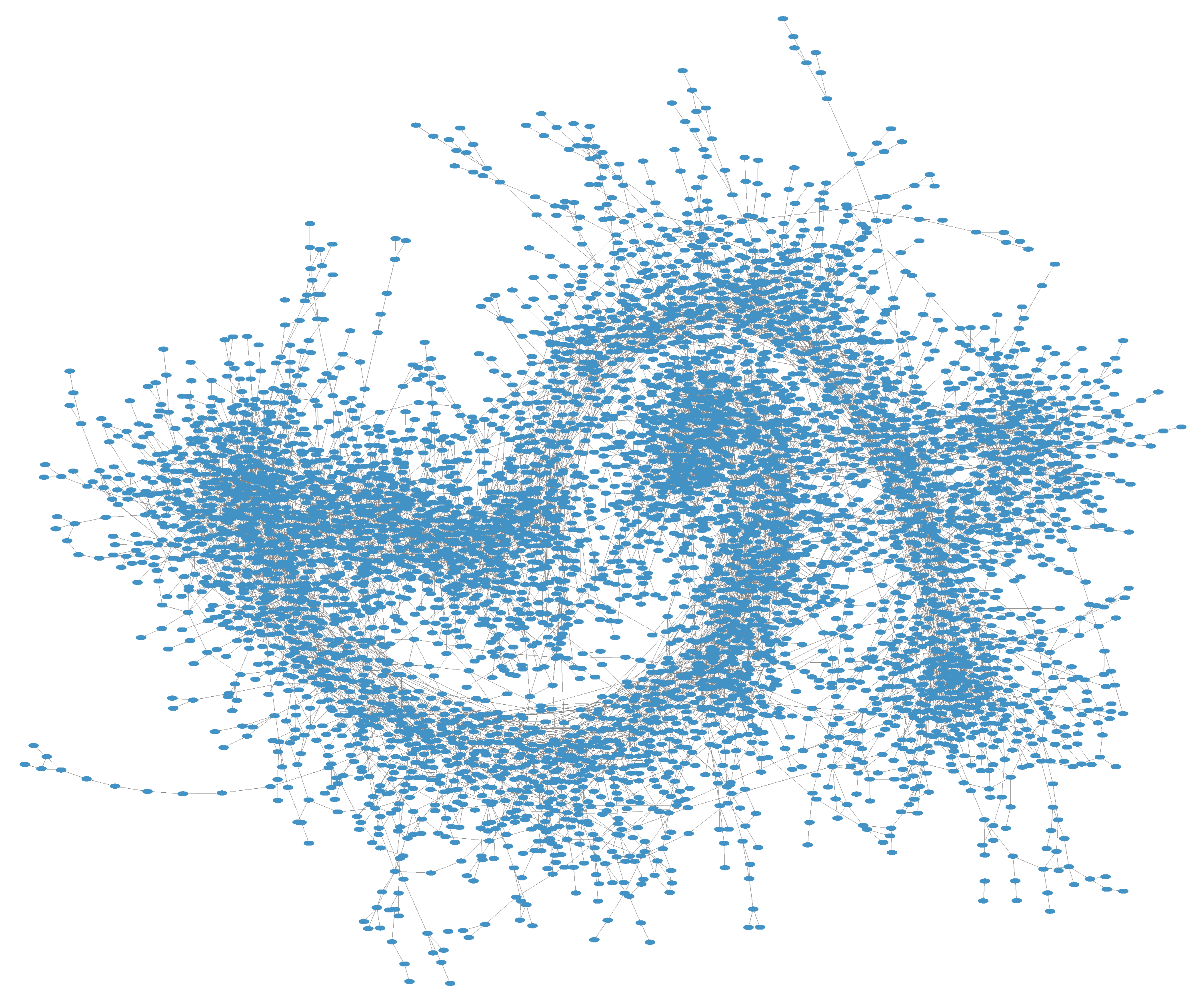
2. Reconstructing and Analysing Interaction Propagation Networks

The basic idea of the approach here proposed is to construct a network representing the potential propagation of interactions between aircraft. Nodes of the network represent aircraft; and a link exists between two nodes whenever the corresponding aircraft have flown closer than a distance ρ . The underlying hypothesis is that, when two aircraft move close to each other, an interaction may occur—usually, the trajectory of one of them (or both) may be changed to avoid a conflict. As a result of this change, one of these aircraft may then move closer than expected to a third one, thus propagating a chain of interactions. A simple illustration of this idea is represented in Figure 1, in which two aircraft a and b interact (i.e., they move closer than a distance threshold ρ , represented by the dotted circles) at time t = 10 min. Afterwards, a third aircraft c enters the airspace, and interacts with aircraft b at time t = 15 min. A more complex network, corresponding to the real trajectories of 1 September 2018, is depicted in Figure A1.
Two important aspects have to be taken into account. Firstly, the temporal characteristic of this network implies that an interaction can only propagate forward in time. To illustrate this aspect with the previous example, the interaction between b and c cannot propagate back to a, as a has already left the area. On the contrary, the interaction between a and b can propagate forward in time to c, as that interaction temporally precedes the bc one. This restriction has to be taken into account when calculating topological metrics on these networks; and is also the main difference with respect to other similar proposals [10,12,13,14], which analyze the networks from a static (as opposed to a temporal) point of view.
Secondly, these networks represent the potential, as opposed to certain, propagation of perturbations. The network representation of the previous example (see bottom right part of Figure 1) indicates that a perturbation can propagate from a to c; in other words, if the trajectory of a is modified, b may also be rerouted to avoid a conflict, which may then require a rerouting of c. This is nevertheless not a certainty. First of all, the perturbation of a’s trajectory may not require a change in b’s, as a may actually be farther away from b; something similar may then apply to the interaction between b and c. Still, pairs of aircraft moving close may generate interactions and these may propagate; the network analysis here proposed is designed to describe the resulting structure. Note that a complementary interpretation is that these networks represent the potential transmission of information between aircraft trajectories.
Once the interaction network has been reconstructed, it is analyzed by means of a set of topological metrics, i.e., values representing several aspects of its structure. Note that, while these are based on metrics that are standard in complex networks theory [15,16,17,18], some of them have been adapted to incorporate the directionality of links—i.e., the network is interpreted as a temporal one [19].
  • Degree. The number of interactions in which one node (i.e., aircraft) is involved. This metric is further synthesized at the network level by calculating the mean degree, i.e., the average number of interactions, and the maximum degree (normalized by the total number of nodes).
  • Isolated nodes. The number of nodes that have experienced no interactions with other nodes, hence for which the degree is zero. It is here expressed as a fraction over the total number of nodes.
  • 2nd/1st degree. The ratio between the degree of the second most connected node of the network, and the degree of the most connected one—i.e., of the second most and most interacting aircraft, respectively. Values close to one indicate that the two most connected nodes have a similar degree, and hence that the network is more homogeneous; conversely, small values suggest that the most connected node is especially well connected.
  • Giant Component. Nodes that compose the largest set of connected nodes. It thus represents the largest set of nodes that are mutually reachable, that is, the largest set of aircraft among which perturbations can propagate. The size of the giant component is here expressed as the fraction of the number of these nodes over the total number of nodes in the network.
  • Entropy of the degree distribution. The entropy S of a probability distribution p ( k ) represents the degree of uncertainty that we have about the values k extracted from it, and is mathematically defined as:
    S = k p ( k ) ln p ( k ) .
    when applied to the distribution of the degrees of nodes, it describes how heterogeneous these are. In other words, the larger S is, the closer the degree distribution is to a uniform one; conversely, when S approaches 0, all aircraft are involved in the same number of interactions. Large values of the entropy thus indicate that the network is more heterogeneous, and this has been proven to be related to its vulnerability [20].
  • Efficiency. The global efficiency of a network is defined as the normalized sum of the inverse of the distances between every pair of nodes [21]:
    E = 1 N ( N 1 ) i j 1 d i j ,
    with N being the total number of nodes. By convention, pairs i , j of aircraft not connected by a path yield 1 / d i j = 0 , and thus do not contribute to the final metric value [21]. The distance d i j is the minimum number of interactions needed to move from aircraft i to aircraft j, taking into account their temporal direction. To illustrate, in Figure 1 the distance between a and c is 2, while the distance between c and a is undefined (due to the temporal dimension, a propagation cannot go from c to a). E is thus defined between 0 and 1, the former indicating that the nodes are completely disconnected, and 1 that a direct link exists between all pairs of nodes. The name comes from the fact that this metric measures how efficient the network is in transmitting information. In the context of this work, the efficiency assesses how easily perturbations are propagated in the system.
  • Diameter. The largest value of the distance between all possible pairs of nodes. In the context of this work, it quantifies the longest possible chain of propagation of interactions.
  • Betweenness centrality. A measure of the centrality of nodes, i.e., how important they are within the network structure. For a given node i, it is proportional to the number of shortest paths connecting every pair of nodes j and k (with j , k i ) that pass through i [22]. Note that the metric is calculated on unweighted networks, i.e., links have no weight (or distance) associated to them. Aircraft with large betweenness centrality play a key role in what is known as the “shortest path structure”, as they are mostly responsible for the propagation of interactions. We here consider two derived metrics: the betweenness centrality of the most central node; and the ratio between the centrality of the second and first most central nodes.
  • Modularity. The magnitude that measures the tendency of a network to organize into communities, i.e., groups of nodes strongly connected between them and loosely connected to the remainder of the network [23,24]. It is calculated as the normalized difference between the actual number of edges that connect nodes of the same community, and the expected number of them (if the network was constructed randomly). Thus, a modularity close to zero implies that the community structure is comparable to that of a random network, i.e., that no significant structure is observed; conversely, a modularity of 1 indicates a structure with disconnected modules. The algorithm here used to calculate the communities is the celebrated Louvain algorithm [25].
  • Vulnerability. This measures how resilient the network is to the elimination of individual nodes [26]; in other words, how much the propagation of perturbations would be hindered if a single aircraft would be excluded from the system. It is calculated by evaluating, for each node, the logarithm of the ratio between the efficiency of the network without that node, and the one of the unaltered network. The smallest value, i.e., the largest loss of efficiency, is taken as the measure of vulnerability of the network.
  • Δ time. Given a propagation network, this metric represents the maximum time a perturbation can propagate in the network. It is thus the temporal equivalent to the diameter.
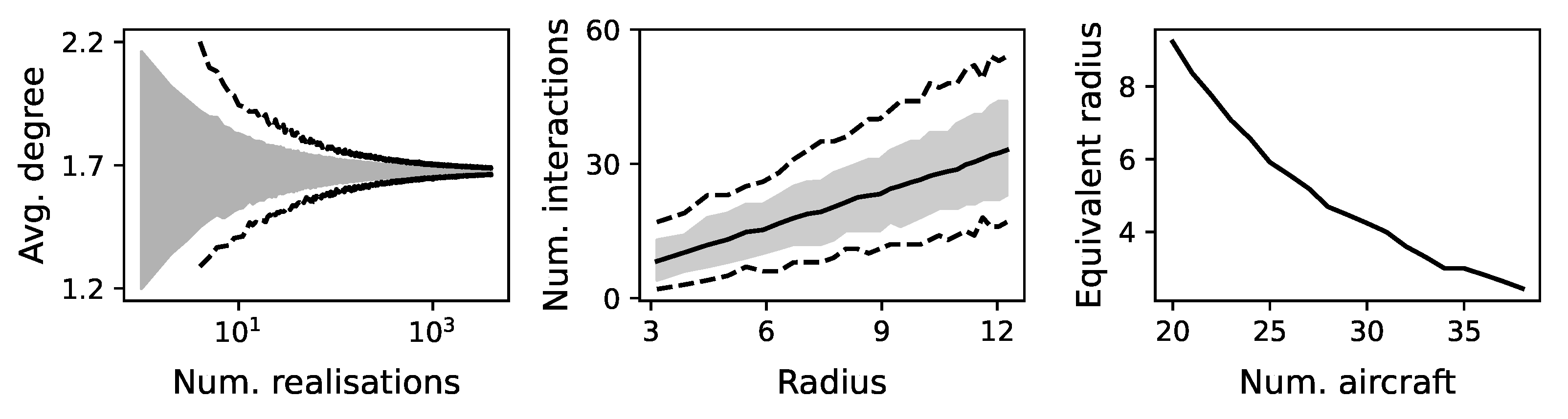
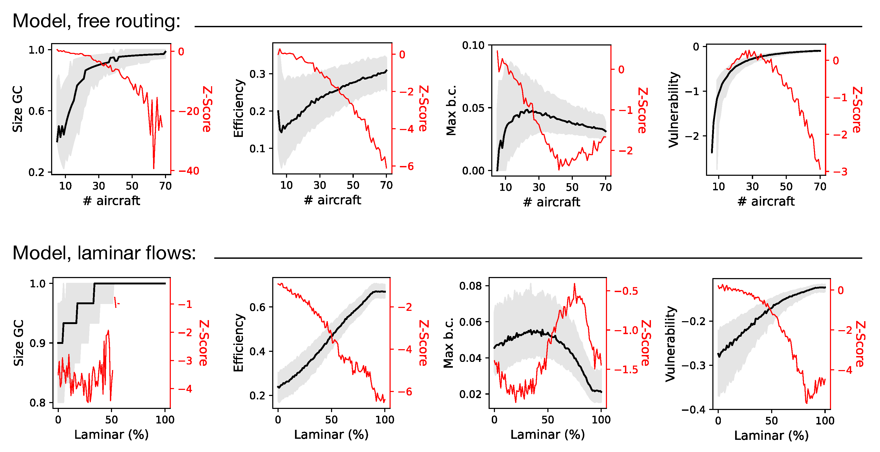
It is important to note that some of these metrics depend on the number of nodes and of links in the network beyond the actual structure they aim at describing. The clearest example is the maximum degree: for the same structure, a network with more links will have a larger maximum degree, and the opposite will happen for a network of the same link density but with more nodes. In order to normalize these metrics, and thus allow comparisons between networks of different sizes, we resort to a null model composed of random equivalent networks; in other words, a set of random networks with the same number of nodes, links, and the same interaction times are created. The original metric is then expressed through the corresponding Z-Score, defined as: z M = ( m r M ¯ ) / σ r M , with r M ¯ and σ r M , respectively, being the mean and standard deviation of the metric M calculated on the random networks. A positive (respectively, negative) value of z M thus indicates that the property measured by the metric M is stronger (weaker) than what is expected in equivalent random networks. It thus allows us to compare different networks, as similar values of z M indicate that the topological property has a similar relevance, irrespectively of the networks’ sizes and densities [27,28].

3. The Model

We start by considering a simple model, in which aircraft are free to fly within a 60 × 60 NM square airspace. N planes enter through any of the sides of the square, at a random time comprised between 0 and 6 min, and with a random direction. The direction is defined through an angle and will be kept constant for the whole trajectory; in other words, we assume that all aircraft fly on a straight trajectory. Aircraft move with a velocity of 600 kn, and their position is recorded every second to constitute their trajectory. We further assume that the space has an Euclidean geometry; in other words, and for the sake of simplicity, we assume a flat surface. A graphical representation of this model is reported in Figure 1, while a list of parameters defining its behavior is available in Table 1.
At each time step, all pairs of aircraft are checked for interactions, specifically by evaluating if their distance is lower than a threshold ρ —note that this parameter acts similar to a radius of interaction. Only pairs of aircraft that have not previously interacted are checked, as by construction aircraft fly according to straight trajectories, and hence cannot diverge then converge again. While this does not necessarily hold for real trajectories, the proportion of pairs of aircraft interacting more than once is less than 3 % , and in most cases these interactions are near in time (see Figure A2); such multiple interactions thus have a minimal impact on the results.
We initially analyze some basic results yielded by the model in Figure 2. First of all, it has to be realized that the model is inherently stochastic, as aircraft paths are defined in a random fashion; as a consequence, multiple realizations of the model with equal parameters have to be executed, in order to extract average metrics. To illustrate this, the left panel reports the evolution of the probability distribution of the average degree, as a function of the number of iterations over which such an average is calculated. It can be appreciated that the dispersion is quite large, requiring 10 3 realizations before a stable result is obtained; hence, all subsequent results correspond to the average over this number of realizations. Afterwards, the central panel of Figure 2 reports the evolution of the number of interactions as a function of the radius ρ ; as is to be expected, the former increases with the latter, in an approximately linear fashion. Finally, the right panel reports the evolution of the radius ρ e required to obtain the same number of interactions as the one obtained for N = 20 aircraft and a radius of ρ = 10 . It is clear that N and ρ are inversely correlated, and that a constant interaction number can be obtained by adjusting them in opposite directions.
We then move to the analysis of some topological metrics, as yielded by the model when varying the number N of aircraft. For the sake of conciseness, four of them are reported in the top panels of Figure 3, while the complete set of results can be found in Figure A3. Introducing more aircraft in the airspace increases the probability for interactions, and hence the size of the giant component and the efficiency; on the other hand, the vulnerability decreases (in absolute value), as new paths for propagation appear and nodes become more redundant. It is nevertheless interesting to see, firstly, that the evolution of the maximum betweenness centrality is not monotonous, reaching a maximum for around 30 aircraft. This is explained by the fact that a low aircraft density prevents perturbation from propagating, and therefore no node is central in such process; on the other hand, a high density makes all aircraft equivalent in importance. Secondly, the Z-Score of the four metrics evolve in an opposite direction (see red lines and right Y axes). This implies that the random networks have larger values of these metrics when compared to the synthetic ones, and the general tendency is for this difference to increase with the number of aircraft. Thus, even if the system seems more efficient in propagating perturbations, it actually becomes less efficient than what would be expected for a random connectivity structure. This is the result of the fact that aircraft have to enter the simulated sector from the borders and that most interactions take place in the center of the airspace—a more efficient propagation could be achieved by evenly distributing aircraft in space.
While the previous model depicts a situation that could be encountered in a free flight airspace, we further study how fixed routes can affect the propagation of interactions. For this, we modify the model by introducing a number λ , defined between 0 % and 100 % , representing how laminar the aircraft flow is. This parameter affects two elements of the model defining how aircraft can enter the airspace. Firstly, it reduces the range of entrance angles, which is now defined as [ λ · π 2 , ( 1 λ 2 ) · π ] . Secondly, it constrains the segments in each side of the square admissible for entrance; being the length of each side 60 NM, the segment is reduced to the range [ 60 · λ 2 , 60 ( 1 λ 2 ) ] . In other words, λ = 1 implies that all aircraft have to enter through the central point of each side of the airspace, and fly on a straight line converging in the center. This thus corresponds to an extreme situation with two bidirectional airways converging in a central waypoint, and “laminar” flows of aircraft. On the other hand, λ = 0 recovers the situation previously presented, with no restrictions applied to aircraft trajectories.
The bottom panels of Figure 3 report the evolution of the previous four topological metrics as a function of λ —the full results are presented in Figure A4. It can be appreciated that the connectivity increases as the flow becomes more laminar, with larger giant components and efficiencies; this is to be expected, as all aircraft have to cross the same central point, and thus cannot avoid interacting. On the other hand, the Z-Scores depict networks that are farther away from random ones, and that are actually less efficient than random graphs. This is due to the structure of interactions imposed by the fact that aircraft are constrained to four converging trajectories. To illustrate this point, imagine two aircraft entering from the same side of the airspace at different times; due to the laminar constraint, they can only interact through a third aircraft flying in the opposite direction. The need for these intermediaries reduces the efficiency of interaction propagation, at least when compared to random networks with no restrictions on the structure.

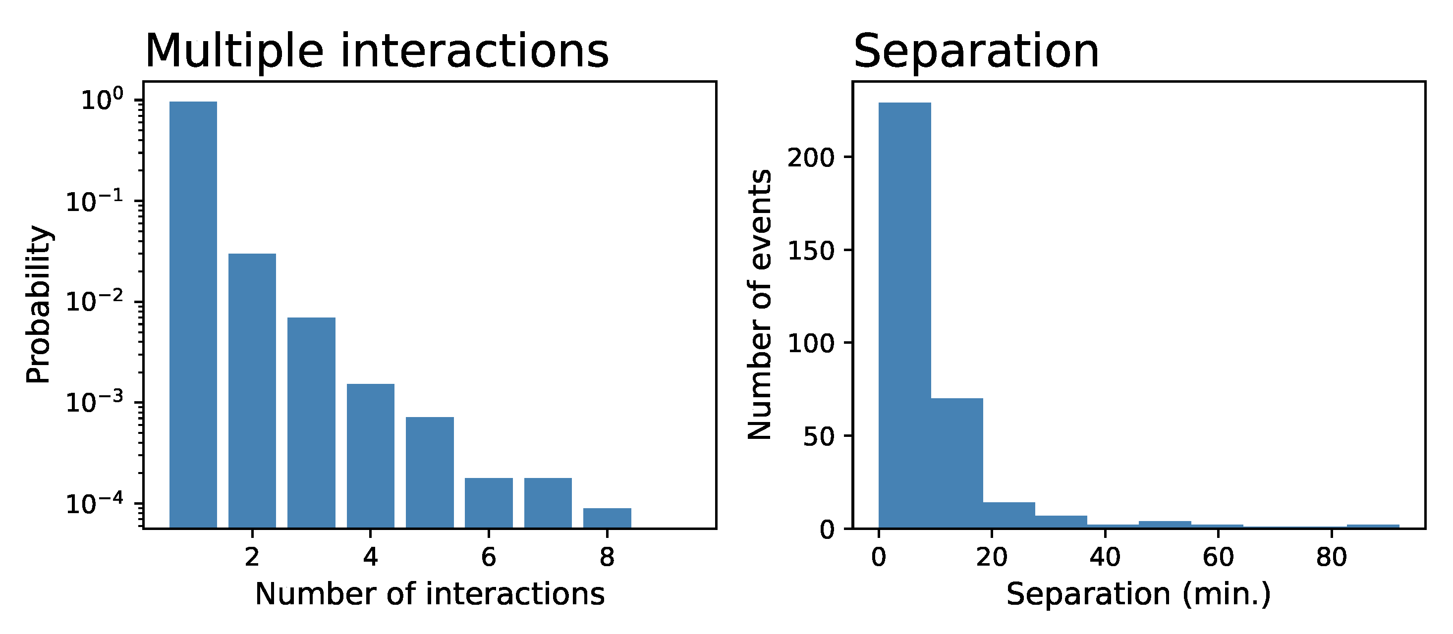
4. Analysis of Real Trajectories

4.1. Trajectory Data and Preprocessing

The data used in this study have been extracted from the EUROCONTROL’s R&D Data Archive, a public repository of historical flights made available for research purposes and freely accessible at https://www.eurocontrol.int/dashboard/rnd-data-archive (accessed on 1 October 2021). It includes information about all commercial flights operating in and over Europe, completed with flight plans, radar data, and the associated airspace structure. The flights considered in this study correspond to four months (i.e., March, June, September and December) of the year 2018 and to September 2015—this latter will be used for assessing the long-term evolution of the system.
For each available flight, two trajectories have been extracted, respectively, the planned (last filed flight plan) and the executed ones. In order to have homogeneous data quality, a rectangular region approximately corresponding to the Maastricht Upper Area Control Centre (MUAC), covering 49–55 degrees of latitude north and 2–11 degrees of longitude east, has been considered, and only the parts of the trajectories included within that airspace have been retained. The trajectories have finally been linearly interpolated, between known points, with a 1-second resolution. Statistics about the data set, including the evolution of the number of trajectories and their time resolution, are reported in Figure A5.

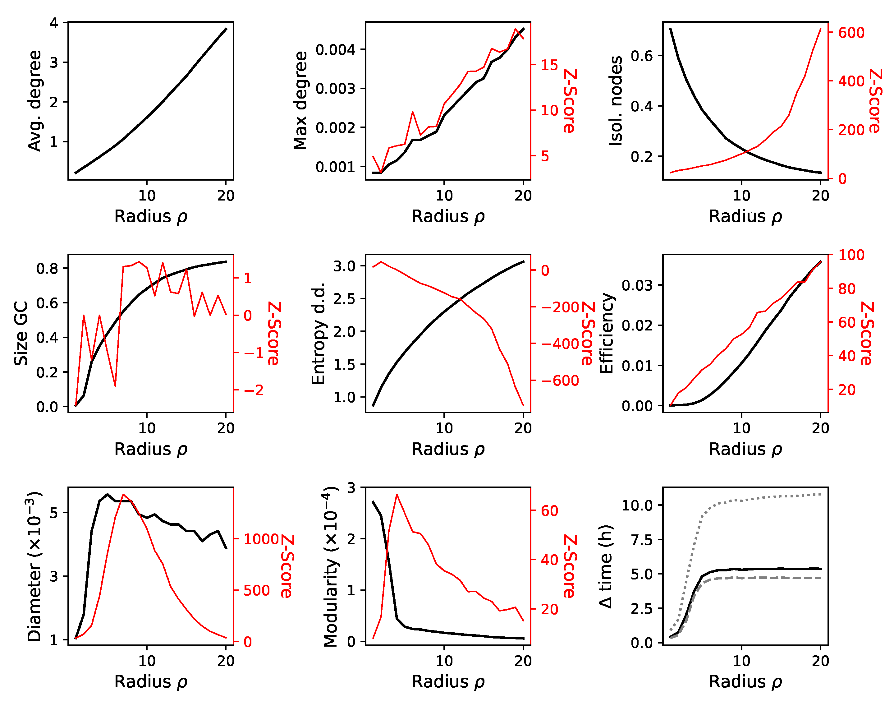
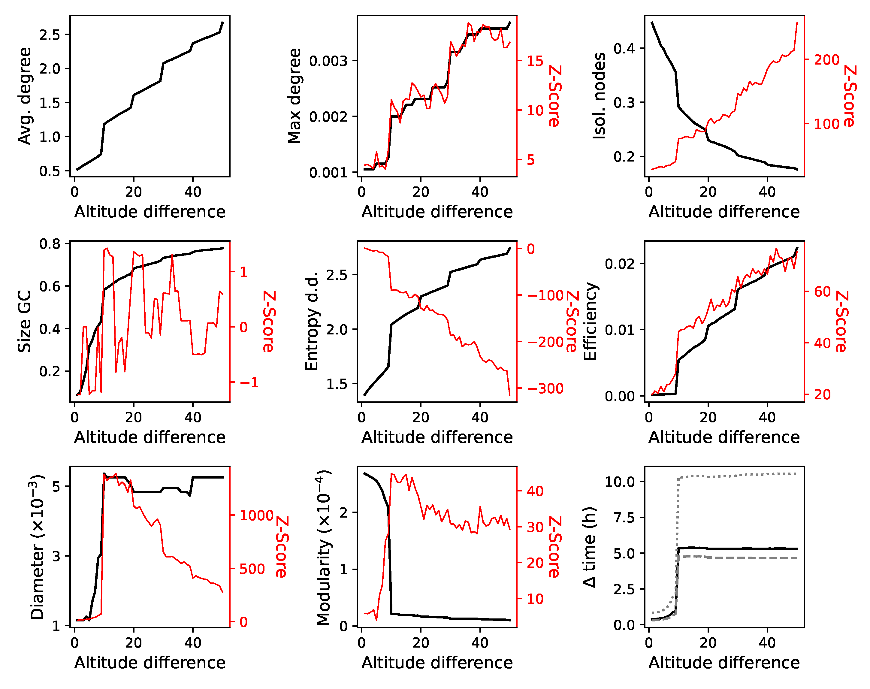
4.2. Basic Results: Interaction Radius and Altitude Difference

In a way similar to what has been presented for the synthetic model, we start by analyzing how the topology changes when two basic reconstruction parameters are varied. For the sake of simplicity, we here consider only the planned trajectories of 1 September 2018. We firstly focus on the radius ρ , i.e., the maximum distance at which we consider that two aircraft are interacting; the selected results are reported in the top panels of Figure 4, and complete results in Figure A6. As is to be expected, the larger this radius, the more aircraft interact. This is nevertheless not a scale-free process: a transition in the topology can be appreciated around 5 NM in the efficiency and in the modularity—a reflection of the 5 NM minimal separation in controlled en route airspace [29].
The bottom panels of Figure 4 (along with Figure A7) further analyze the evolution of the interaction network as a function of the maximum altitude difference allowed between two aircraft to accept the existence of an interaction. Note that this aspect was not simulated in the synthetic model, as aircraft were considered to fly at the same altitude; but is instead an essential ingredient of real traffic. The structure imposed by airways, and more specifically the requirement of flying at specific flight levels, is evident in the results, with strong transitions at 1000, 2000, and 3000 feet.
The results presented in Figure 4 have also been used to fix the values of these two parameters in subsequent analyses. In order to represent the system in a stable phase, i.e., away from the major transitions previously described, we will from now on fix the radius ρ to 10 NM and the altitude difference to 2000 feet (or 20 flight levels). Note that the chosen radius is larger than the en route separation minima; this allows us to detect interactions before these become conflicts, thus when they are not yet a safety hazard, but still require the intervention of air traffic controllers.

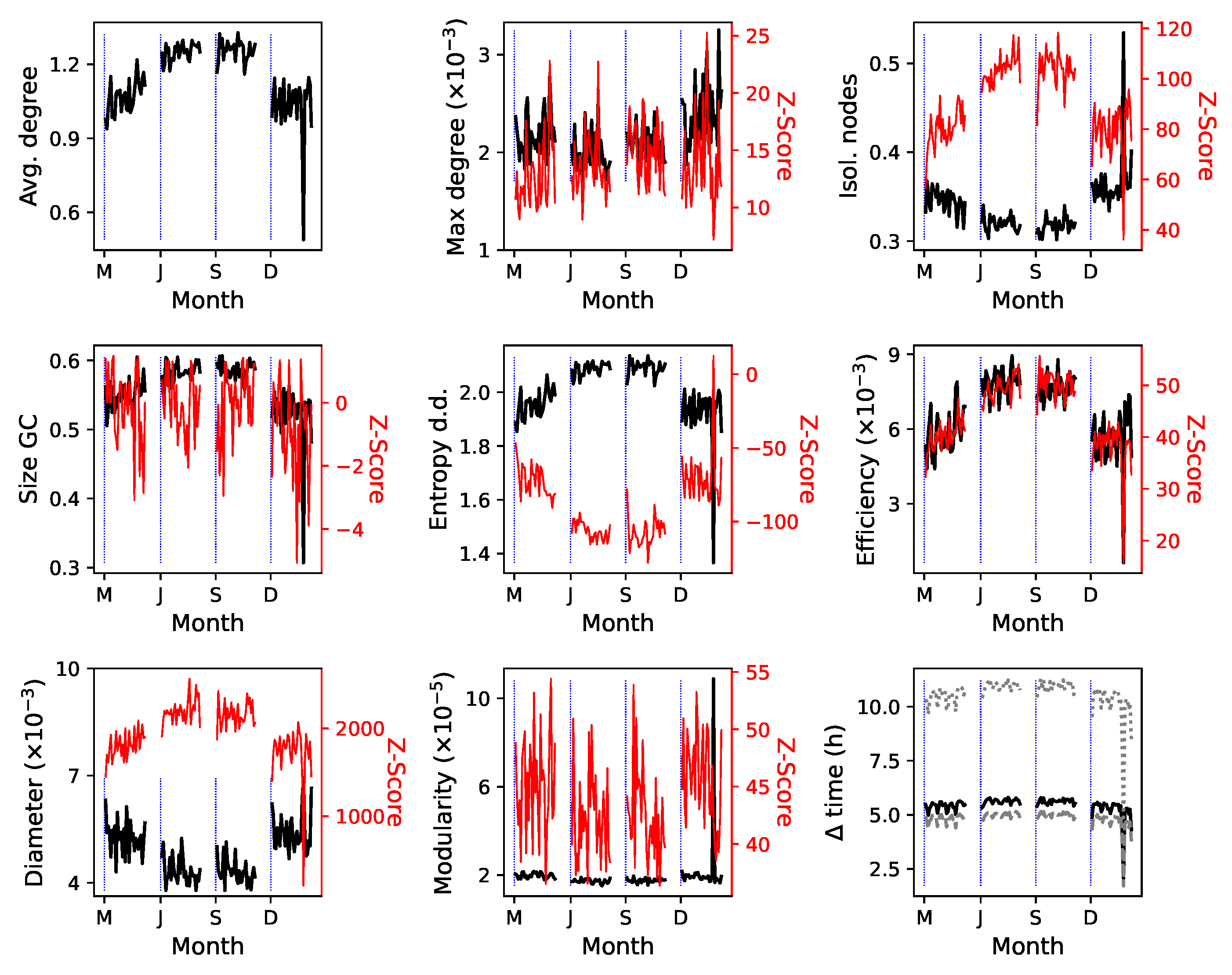
4.3. Properties of Planned and Executed Trajectories

We delve deeper in the analysis of the properties of the real interaction networks by considering the evolution through time of the resulting topological metrics for planned trajectories—see the top panels of Figure 5 and Figure A8. The Z-Scores of the topological metrics describe networks with some general and stable properties. Specifically, the high number of isolated nodes and the extremely low entropy of the degree distribution (see corresponding Z-Scores) imply that most interactions are centered around a few hub nodes (i.e., flights), with the majority experiencing few or no interactions. The modularity is also large, thus suggesting that the network is organized in weakly connected groups of nodes, each one centered around one hub. This modular hub-and-spoke structure implies, on one hand, that perturbations can easily move between the nodes that are part of a community—note the high efficiency; at the same time, crossing the whole network requires jumping between multiple communities, hence the large diameter. In synthesis, the perturbations easily propagate on a local scale, but are prevented from spreading to the whole system.
Additionally, the modular hub-and-spoke structure is accentuated during the months of June and September—especially in the case of the number of isolated nodes, entropy of the degree distribution, and efficiency. Note that this is not the result of the increased volume of traffic characteristics of these months, as the use of a Z-Score ensures that the metrics are normalized, independently on the number of interactions; in other words, they only describe the structure of the network. On the contrary, the results suggest that the structure is caused by the changes of traffic patterns common in summer, with flights connecting more touristic destinations in the Mediterranean sea, and spending less time in the central (and more congested) part of Europe.
We then move to the analysis of the structure of the interaction networks observed during operations, i.e., according to the executed trajectories, see the bottom panels of Figure 5 and Figure A9. When compared to planned trajectories, it can firstly be noted that the average degree (and hence the number of interactions) is smaller—see also Figure 6 for a scatter plot comparing planned and executed trajectories. This is to be expected, as this is the main duty of air traffic controllers. Additionally, several topological metrics have lower absolute values: the number of isolated nodes, the entropy of the degree distribution, and the efficiency; on the contrary, diameter and modularity present higher values. In other words, while reducing interactions, air traffic controllers are affecting the network. The result is a topology with a more marked modular structure, and with a hindered propagation of interactions among distant parts of the network.
We further analyze how the interaction network has evolved through the years, by comparing the values of the topological metrics for September 2015 and 2018. Specifically, Figure 7 reports the Z-Score of the four metrics that have most changed; see also Figure A10 for a complete analysis of the executed trajectories for September 2015. With the exception of the modularity, all other metrics have increased in absolute value, indicating that the network was less random in 2018 when compared to 2015. Note that the Z-Score normalizes the metrics according to the size of the network; hence, the change in topology is not the direct result of the higher volume of traffic observed in year 2018. On the contrary, this may be the result of changes in the structure of air routes over these four years [30]. It is also worth noting that, while the number of isolated nodes increased in 2018, so did the efficiency. In other words, more aircraft are able to fly without interacting with others; but, at the same time, those that interact do so in a tighter way, enabling a stronger propagation within the core of the network.

4.4. Robustness of the Interaction Network

As a final point, we analyze how robust the structure of the interaction propagation networks is to targeted perturbations, with the aim of understanding how easy would it be to change their structure. In other words, one may ask how many trajectories have to be changed in order to significantly disrupt the propagation of perturbations. While a complete analysis is unfeasible due to the size of the network, we here resort to an iterative pruning process. Starting from the original network of 1 September 2018, for executed trajectories, the node with the largest number of interactions is chosen (or one at random in case of a tie), and one of its links is deleted at random; the process is repeated until the desired number of links are removed.
The evolution of the number of isolated nodes, efficiency and modularity as a function of the number of deleted interactions is reported in Figure 8, while complete results can be found in Figure A11. It can be appreciated that deleting a few hundred interactions, which corresponds to approximatively isolating a few tens of flights, is enough to change the Z-Score by 10 % , thus significantly altering the topology. Additionally, the efficiency is strongly lowered; the propagation is thus hindered more than what is obtained if the interactions were deleted at random (dotted red lines of Figure 8), as expected. Simultaneously, the modularity is increased; this suggests that the most interacting aircraft are also responsible for connecting groups of flights that would otherwise be less coupled.

5. Discussion and Conclusions

In this contribution, we have proposed a way of mapping potential interactions between aircraft in a network structure, which describes how such interactions can propagate, and their long-term cascading effects. By leveraging on some simplifications, such as, e.g., deviations from planned trajectories are not simulated, it enables analyses for long time horizons, and is thus not limited to a single sector or a single conflict. We firstly showed how the approach works by considering a simplified (or toy model) airspace, where parameters such as the number of aircraft and their trajectories can be fully tuned (see Figure 3). The approach has then been applied to flights crossing a large European airspace in 2018, highlighting the topologies induced by airway structures (Figure 4); the differences between planned and executed trajectories, i.e., the effects of air traffic controllers’ interventions (Figure 6); the evolution of such networks through time (Figure 5 and Figure 7); and their robustness, i.e., how difficult it is to hinder the propagation of such interactions (Figure 8). While, for the sake of clarity and conciseness, only basic results are shown in these figures, the interested reader can find extensive results in the appendices.
While this is the first time the concept of interaction networks is proposed, several interesting applications can be foreseen. First of all, and as here illustrated, the topological properties of the network can be used to monitor the behavior of the system, by analyzing the trajectories of the past days and the evolution of the network structure they induced. This could be used to detect anomalous behaviors, or to track the reaction of the system to exogenous events, such as, e.g., strikes or other large-scale disruptions [31]. The distances between pairs of aircraft may also be key in future technologies, such as air-to-air communication schemes [32]. Beyond descriptive applications, the concept of interaction networks can also be applied in predictive studies. To illustrate, the network manager may use planned trajectories to evaluate the structure of the interaction network a few days in advance [33], and to suggest (or impose) reroutings in the event of strong propagations. This is supported by the fact that avoiding a small number of critical interactions can significantly affect the structure of the network, as seen in Figure 8. This can also be performed on a smaller time and spatial scale, e.g., to warn air traffic controllers about the development of complex situations. In synthesis, the network representation can be used as an ingredient to evaluate and forecast air traffic controller workloads [34,35,36]. Finally, we foresee that the proposed approach could be useful in the training of air traffic controllers; to illustrate, a student can be required to manage a complex traffic scenario, possibly created using the proposed synthetic model, with the interaction network being a way to evaluate the quality of his/her solution. A similar evaluation could also be applied to automatic conflict detection and resolution algorithms [37,38,39].
Before any real-world application of this approach can be deployed, more research is needed on three key aspects. Firstly, topological metrics cannot substitute the experience of air traffic controllers, and the former ones should rather be validated by the latter. To illustrate, the efficiency of the network is intuitively representative of the easiness with which perturbations can propagate. Yet, this shall experimentally be validated, by comparing different real traffic scenarios; and controllers may further find some smaller-scale metrics (e.g., the average degree) more useful and easier to explain. Secondly, the parameters used in the reconstruction of the network, and especially the separation radius ρ , have here been defined arbitrarily. This could be solved, on one hand, by using real separation minima, or any other operational criteria, provided the trajectory data have a high enough resolution; but also by reconstructing a multi-layer network [40,41], in which each layer represents the topology obtained through a different ρ , thus yielding a more complete depiction of the interactions. Thirdly, the analysis of the robustness has here been simplified through a pruning process. It has to be noted that more sophisticated algorithms for network dismantling are available, albeit usually with a higher computational cost—see [42] for a review and comparison. Additionally, assuming that a link (i.e., an interaction) can simply be deleted is an oversimplification; instead, interactions should be avoided by modifying the involved trajectories, a process that can be computationally complex.
All these potential applications must be evaluated in the light of a significant drawback of this method, i.e., its non-negligible computational cost. To illustrate, the reconstruction and analysis of one of the networks here presented required tens of hours—see Figure A13 for a full analysis as a function of the number of flights. As a consequence, the application of this approach to, e.g., the analysis of the complete European airspace and of all flights of one day would require the development of optimized software solutions, possibly relying on parallelized hardware architectures. While possible, the analysis of such large problems is not a trivial endeavor. Still, applying this method to individual sectors, with, e.g., tens of trajectories, is feasible even in scenarios requiring near real-time results.

Author Contributions

Conceptualization, M.Z.; formal analysis, R.L.-M.; data curation, R.L.-M.; writing—original draft preparation, R.L.-M. and M.Z.; writing—review and editing, R.L.-M. and M.Z. All authors have read and agreed to the published version of the manuscript.

Funding

This project has received funding from the European Research Council (ERC) under the European Union’s Horizon 2020 research and innovation programme (grant agreement No. 851255). This work has been partially supported by the María de Maeztu project CEX2021-001164-M funded by the MCIN/AEI/10.13039/501100011033. R.L.-M. acknowledges funding from CSIC, JAE program.

Data Availability Statement

The data that support the findings of this study are openly available at https://www.eurocontrol.int/dashboard/rnd-data-archive (accessed on 1 October 2021).

Conflicts of Interest

The authors declare no conflict of interest.

Appendix A

Figure A1. Graphical representation of the giant connected component of the network of interactions, for executed trajectories of 1 September 2018. Links represent instances in which the corresponding pair of aircraft interacted, i.e., their horizontal separation was less than ρ = 10 NM and the vertical distance less than 2000 feet. Picture created in Cytoscape 3.8 with yFiles Organic Layout embedding, © Cytoscape Consortium.
Aerospace 10 00213 g0a1
Figure A2. Analysis of the cases in which pairs of aircraft undergo multiple interactions. The left panel reports, for the executed trajectories of 1 September 2018, the probability of finding pairs of aircraft interacting multiple times, for ρ = 10 NM and a vertical separation of 2000 feet. The right panel depicts a histogram of the time separation, in min, between consecutive interactions, for those pairs of aircraft that have interacted twice.
Aerospace 10 00213 g0a2
Figure A3. Evolution of the topological metrics yielded by the synthetic model, in the free routing condition, as a function of the number of aircraft. Black (left Y axes) and red lines (right Y axes), respectively, correspond to the raw values of the metrics and their Z-Scores. Grey bands correspond to the 10–90 percentiles.
Aerospace 10 00213 g0a3
Figure A4. Evolution of the topological metrics yielded by the synthetic model, in the laminar condition, as a function of the laminar constraint λ . Black (left Y axes) and red lines (right Y axes), respectively, correspond to the raw values of the metrics and their Z-Scores. Grey bands correspond to the 10–90 percentiles.
Aerospace 10 00213 g0a4
Figure A5. Statistics of the flights for 2018. From top to bottom, the five panels, respectively, report: the number of flights crossing the considered airspace; the distribution of the temporal resolution, i.e., of the time, in seconds, between available points, for planned and executed trajectories; and the distribution of the reported altitude, also for planned and executed trajectories. In the last four panels, black and red lines, respectively, correspond to planned and executed trajectories. Solid lines further correspond to the median of the daily value, dashed lines to the average, and bands to the 10–90 percentile.
Aerospace 10 00213 g0a5aAerospace 10 00213 g0a5b
Figure A6. Properties of the interaction networks, for the planned trajectories of 1 September 2018, as a function of the interaction radius ρ . Black (left Y axes) and red lines (right Y axes), respectively, correspond to the raw values and their Z-Scores.
Aerospace 10 00213 g0a6
Figure A7. Properties of the interaction networks, for the planned trajectories of 1 September 2018 and ρ = 10 NM, as a function of the altitude difference. Black (left Y axes) and red lines (right Y axes), respectively, correspond to the raw values and their Z-Scores.
Aerospace 10 00213 g0a7
Figure A8. Properties of the interaction networks for planned trajectories in 2018. Each panel depicts the evolution through time of a topological metric, as defined in Section 2; black (left Y axes) and red lines (right Y axes), respectively, correspond to the raw values and their Z-Scores. The vertical blue dotted lines represent the beginning of each month. In the last panel, the black line corresponds to the median, the gray dashed one to the mean, and the gray dotted one to the maximum. M: March; J: June; S: September; and D: December.
Aerospace 10 00213 g0a8
Figure A9. Properties of the interaction networks for executed trajectories in 2018. Each panel depicts the evolution through time of a topological metric, as defined in Section 2; black (left Y axes) and red lines (right Y axes), respectively, correspond to the raw values and their Z-Scores. The vertical blue dotted lines represent the beginning of each month. In the last panel, the black line corresponds to the median, the gray dashed one to the mean, and the gray dotted one to the maximum. M: March; J: June; S: September; and D: December.
Aerospace 10 00213 g0a9
Figure A10. Properties of the interaction networks for executed trajectories, corresponding to September 2015. Each panel depicts the evolution through time of a topological metric, as defined in Section 2; black (left Y axes) and red lines (right Y axes), respectively, correspond to the raw values and their Z-Scores. In the last panel, the black line corresponds to the median, the gray dashed one to the mean, and the gray dotted one to the maximum.
Aerospace 10 00213 g0a10
Figure A11. Properties of the interaction network for executed trajectories of 1 September, subject to a pruning process. Metrics are reported as a function of the number of deleted links—see the main text for details on the pruning algorithm. Black (left Y axes) and red lines (right Y axes), respectively, correspond to the raw values and their Z-Scores.
Aerospace 10 00213 g0a11
Figure A12. Properties of the interaction network for executed trajectories of 1 September, subject to a random pruning process. Metrics are reported as a function of the number of deleted links, with links being deleted at random. Black (left Y axes) and red lines (right Y axes), respectively, correspond to the raw values and their Z-Scores.
Aerospace 10 00213 g0a12
Figure A13. Computational cost. The left and right panels, respectively, depict the evolution of the computational cost (in seconds) for reconstructing the interaction network and its topological analysis, as a function of the number of flights included in it. Results have been obtained by taking the executed trajectories corresponding to 3 September 2018 (i.e., the day with the highest volume of traffic), and deleting a random part of them. Calculations have been performed on a server with AMD Epyc2 7402 processors (limited to a single core) and 64 GB of memory.
Aerospace 10 00213 g0a13

References

  1. Nolan, M.S. Fundamentals of Air Traffic Control; Cengage Learning: Belmont, CA, USA, 2011. [Google Scholar]
  2. Galster, S.M.; Duley, J.A.; Masalonis, A.J.; Parasuraman, R. Air traffic controller performance and workload under mature free flight: Conflict detection and resolution of aircraft self-separation. Int. J. Aviat. Psychol. 2001, 11, 71–93. [Google Scholar] [CrossRef]
  3. Radanovic, M.; Eroles, M.A.P.; Koca, T.; Gonzalez, J.J.R. Surrounding traffic complexity analysis for efficient and stable conflict resolution. Transp. Res. Part C Emerg. Technol. 2018, 95, 105–124. [Google Scholar] [CrossRef]
  4. Jun, T.; Piera, M.A.; Ruiz, S. A causal model to explore the ACAS induced collisions. Proc. Inst. Mech. Eng. Part G J. Aerosp. Eng. 2014, 228, 1735–1748. [Google Scholar] [CrossRef]
  5. Lizarraga, M.; Elkaim, G. Spatially deconflicted path generation for multiple UAVs in a bounded airspace. In Proceedings of the 2008 IEEE/ION Position, Location and Navigation Symposium, Monterey, CA, USA, 5–8 May 2008; IEEE: New York, NY, USA, 2008; pp. 1213–1218. [Google Scholar]
  6. Gariel, M.; Srivastava, A.N.; Feron, E. Trajectory clustering and an application to airspace monitoring. IEEE Trans. Intell. Transp. Syst. 2011, 12, 1511–1524. [Google Scholar] [CrossRef] [Green Version]
  7. Gardi, A.; Sabatini, R.; Ramasamy, S.; Kistan, T. Real-time trajectory optimisation models for next generation air traffic management systems. Appl. Mech. Mater. Trans. Tech. Publ. 2014, 629, 327–332. [Google Scholar] [CrossRef]
  8. Wei, J.; Sciandra, V.; Hwang, I.; Hall, W.D. Design and evaluation of a dynamic sectorization algorithm for terminal airspace. J. Guid. Control. Dyn. 2014, 37, 1539–1555. [Google Scholar] [CrossRef]
  9. Schuster, H.G.; Just, W. Deterministic Chaos: An Introduction; John Wiley & Sons: New York, NY, USA, 2006. [Google Scholar]
  10. Zanin, M. Network analysis reveals patterns behind air safety events. Phys. A Stat. Mech. Its Appl. 2014, 401, 201–206. [Google Scholar] [CrossRef]
  11. Monechi, B.; Servedio, V.D.; Loreto, V. Congestion transition in air traffic networks. PLoS ONE 2015, 10, e0125546. [Google Scholar] [CrossRef]
  12. Zhang, J.; Yang, J.; Wu, C. From trees to forest: Relational complexity network and workload of air traffic controllers. Ergonomics 2015, 58, 1320–1336. [Google Scholar] [CrossRef]
  13. Wang, H.; Song, Z.; Wen, R.; Zhao, Y. Study on evolution characteristics of air traffic situation complexity based on complex network theory. Aerosp. Sci. Technol. 2016, 58, 518–528. [Google Scholar] [CrossRef]
  14. Wang, H.; Song, Z.; Wen, R. Modeling air traffic situation complexity with a dynamic weighted network approach. J. Adv. Transp. 2018, 2018, 5254289. [Google Scholar] [CrossRef] [Green Version]
  15. Albert, R.; Barabási, A.L. Statistical mechanics of complex networks. Rev. Mod. Phys. 2002, 74, 47. [Google Scholar] [CrossRef] [Green Version]
  16. Boccaletti, S.; Latora, V.; Moreno, Y.; Chavez, M.; Hwang, D.U. Complex networks: Structure and dynamics. Phys. Rep. 2006, 424, 175–308. [Google Scholar] [CrossRef]
  17. Newman, M.E. The structure and function of complex networks. SIAM Rev. 2003, 45, 167–256. [Google Scholar] [CrossRef] [Green Version]
  18. Costa, L.D.F.; Rodrigues, F.A.; Travieso, G.; Villas Boas, P.R. Characterization of complex networks: A survey of measurements. Adv. Phys. 2007, 56, 167–242. [Google Scholar] [CrossRef] [Green Version]
  19. Holme, P.; Saramäki, J. Temporal networks. Phys. Rep. 2012, 519, 97–125. [Google Scholar] [CrossRef] [Green Version]
  20. Wang, B.; Tang, H.; Guo, C.; Xiu, Z. Entropy optimization of scale-free networks’ robustness to random failures. Phys. A Stat. Mech. Its Appl. 2006, 363, 591–596. [Google Scholar] [CrossRef] [Green Version]
  21. Latora, V.; Marchiori, M. Efficient behavior of small-world networks. Phys. Rev. Lett. 2001, 87, 198701. [Google Scholar] [CrossRef] [Green Version]
  22. Barthelemy, M. Betweenness centrality in large complex networks. Eur. Phys. J. B 2004, 38, 163–168. [Google Scholar] [CrossRef]
  23. Fortunato, S. Community detection in graphs. Phys. Rep. 2010, 486, 75–174. [Google Scholar] [CrossRef] [Green Version]
  24. Lambiotte, R.; Schaub, M.T. Modularity and Dynamics on Complex Networks; Cambridge University Press: Cambridge, UK, 2021. [Google Scholar]
  25. Blondel, V.D.; Guillaume, J.L.; Lambiotte, R.; Lefebvre, E. Fast unfolding of communities in large networks. J. Stat. Mech. Theory Exp. 2008, 2008, P10008. [Google Scholar] [CrossRef] [Green Version]
  26. Holme, P.; Kim, B.J.; Yoon, C.N.; Han, S.K. Attack vulnerability of complex networks. Phys. Rev. E 2002, 65, 056109. [Google Scholar] [CrossRef] [PubMed] [Green Version]
  27. Maslov, S.; Sneppen, K. Specificity and stability in topology of protein networks. Science 2002, 296, 910–913. [Google Scholar] [CrossRef] [PubMed] [Green Version]
  28. Zanin, M.; Sun, X.; Wandelt, S. Studying the topology of transportation systems through complex networks: Handle with care. J. Adv. Transp. 2018, 2018, 3156137. [Google Scholar] [CrossRef] [Green Version]
  29. Halpern, N.; Graham, A. The Routledge Companion to Air Transport Management; Routledge: London, UK, 2018. [Google Scholar]
  30. Sun, X.; Wandelt, S.; Linke, F. Temporal evolution analysis of the European air transportation system: Air navigation route network and airport network. Transp. B Transp. Dyn. 2015, 3, 153–168. [Google Scholar] [CrossRef]
  31. Basora, L.; Olive, X.; Dubot, T. Recent advances in anomaly detection methods applied to aviation. Aerospace 2019, 6, 117. [Google Scholar] [CrossRef] [Green Version]
  32. Ho, T.; Shigeru, S. Mobile Ad-Hoc Network Based Relaying Data System for Oceanic Flight Routes in Aeronautical Communications. Int. J. Comput. Netw. Commun. 2009, 1, 10803862. [Google Scholar]
  33. Murca, M.C.R.; Hansman, R.J. Identification, characterization, and prediction of traffic flow patterns in multi-airport systems. IEEE Trans. Intell. Transp. Syst. 2018, 20, 1683–1696. [Google Scholar] [CrossRef]
  34. Chatterji, G.; Sridhar, B. Measures for air traffic controller workload prediction. In Proceedings of the 1st AIAA, Aircraft, Technology Integration, and Operations Forum, Los Angeles, CA, USA, 16–18 October 2001; p. 5242. [Google Scholar]
  35. Hilburn, B. Cognitive complexity in air traffic control: A literature review. EEC Note 2004, 4, 1–80. [Google Scholar]
  36. Loft, S.; Sanderson, P.; Neal, A.; Mooij, M. Modeling and predicting mental workload in en route air traffic control: Critical review and broader implications. Hum. Factors 2007, 49, 376–399. [Google Scholar] [CrossRef] [Green Version]
  37. Durand, N.; Alliot, J.M.; Noailles, J. Automatic aircraft conflict resolution using genetic algorithms. In Proceedings of the 1996 ACM Symposium on Applied Computing, Philadelphia, PA, USA, 17–19 February 1996; pp. 289–298. [Google Scholar]
  38. Cafieri, S.; Durand, N. Aircraft deconfliction with speed regulation: New models from mixed-integer optimization. J. Glob. Optim. 2014, 58, 613–629. [Google Scholar] [CrossRef] [Green Version]
  39. Courchelle, V.; Soler, M.; González-Arribas, D.; Delahaye, D. A simulated annealing approach to 3D strategic aircraft deconfliction based on en-route speed changes under wind and temperature uncertainties. Transp. Res. Part C Emerg. Technol. 2019, 103, 194–210. [Google Scholar] [CrossRef]
  40. Kivelä, M.; Arenas, A.; Barthelemy, M.; Gleeson, J.P.; Moreno, Y.; Porter, M.A. Multilayer networks. J. Complex Netw. 2014, 2, 203–271. [Google Scholar] [CrossRef] [Green Version]
  41. Boccaletti, S.; Bianconi, G.; Criado, R.; Del Genio, C.I.; Gómez-Gardenes, J.; Romance, M.; Sendina-Nadal, I.; Wang, Z.; Zanin, M. The structure and dynamics of multilayer networks. Phys. Rep. 2014, 544, 1–122. [Google Scholar] [CrossRef] [Green Version]
  42. Wandelt, S.; Sun, X.; Feng, D.; Zanin, M.; Havlin, S. A comparative analysis of approaches to network-dismantling. Sci. Rep. 2018, 8, 13513. [Google Scholar] [CrossRef] [Green Version]
Figure 1. Example of the reconstruction of the network of interactions. The three panels represent an airspace at three different moments in time ( t = 5 , 10 and 15 min), with three aircraft crossing it. An interaction between two aircraft is detected when their respective distance is smaller than a threshold ρ , depicted as dotted circles. The bottom right panel reports the resulting interaction network; note that links have a time stamp associated to them, as we assume that interactions cannot back-propagate in time (in this case, the interaction between b and c cannot propagate to a).
Aerospace 10 00213 g001
Figure 2. Basic analysis of the synthetic model. (Left) Distribution of the obtained average degree as a function of the number of realizations. The gray band and the black dashed lines, respectively, represent the 10–90 and the 1–99 percentiles. (Center) Evolution of the number of interactions as a function of the radius ρ , for N = 20 aircraft. The black solid line reports the average, while the gray band and the dashed black lines, respectively, represent the 10–90 and the 1–99 percentiles. (Right) Evolution of the equivalent radius ρ e needed to recover the same number of interactions, as obtained for N = 20 and ρ = 10 , as a function of the number of simulated aircraft.
Aerospace 10 00213 g002
Figure 3. Properties of the interaction networks yielded by the synthetic model, for the free routing (top panels) and the laminar flow (bottom panel) cases. See Figure A3 and Figure A4 for full results. Black (left Y axes) and red lines (right Y axes), respectively, correspond to the raw values of the metrics and their Z-Scores. Grey bands correspond to the 10–90 percentiles. A radius of interactions ρ = 10 NM was used in the free routing case; N = 30 and ρ = 10 NM in the laminar flows analysis.
Aerospace 10 00213 g003
Figure 4. Properties of the interaction networks for the planned trajectories of 1 September 2018, as a function of the interaction radius ρ (in nautical miles, top panels) and the altitude difference (in hundreds of feet, bottom panels). See Figure A6 and Figure A7 for full results. Black (left Y axes) and red lines (right Y axes), respectively, correspond to the raw values of the metrics and their Z-Scores.
Aerospace 10 00213 g004
Figure 5. Properties of the interaction networks for planned (top panels) and executed (bottom panels) trajectories, as a function of time. See Figure A8 and Figure A9 for full results. Black (left Y axes) and red lines (right Y axes), respectively, correspond to the raw values of the metrics and their Z-Scores. The vertical blue dotted lines represent the beginning of each month. M: March; J: June; S: September; D: December.
Aerospace 10 00213 g005
Figure 6. Comparing planned and executed operations. Each panel depicts a scatter plot of a network metric, for the executed operations and as a function of the planned ones. Colors of points indicate the respective month, see legend in the first panel. Note that only metrics with a significant Z-Score are here reported. With the exception of the average degree, all values correspond to the Z-Score of the metric.
Aerospace 10 00213 g006
Figure 7. Comparing executed operations in September 2015 and 2018. Each panel depicts the evolution of a network metric for the years 2015 (blue lines) and 2018 (black lines), as a function of the day of the month—see Figure A10 for a complete analysis of the 2015 networks.
Aerospace 10 00213 g007
Figure 8. Properties of the interaction networks subject to a pruning process, as a function of the number of deleted links. See Figure A11 for full results, and the main text for a description of the pruning strategy. Solid black (left Y axes) and red lines (right Y axes), respectively, correspond to the raw values of the metrics and the associated Z-Scores. Dotted red lines (right Y axes) report the Z-Scores of the metrics in the case of a random pruning process—see the full results in Figure A12.
Aerospace 10 00213 g008
Table 1. List of parameters defining the behavior of the synthetic model, and description of their meaning.
ParameterMeaning
NNumber of simulated aircraft.
ρ Radius of interaction, i.e., the distance below which a pair of aircraft is assumed to be interacting.
λ Laminar percentage, defining how constrained (in terms of the entrance spatial window and angle) the aircraft entrance to the airspace is.
Disclaimer/Publisher’s Note: The statements, opinions and data contained in all publications are solely those of the individual author(s) and contributor(s) and not of MDPI and/or the editor(s). MDPI and/or the editor(s) disclaim responsibility for any injury to people or property resulting from any ideas, methods, instructions or products referred to in the content.

