
Evaluation of Large-Eddy Simulation Coupled with an Homogeneous Equilibrium Model for the Prediction of Coaxial Cryogenic Flames under Subcritical Conditions

Abstract
:1. Introduction
2. Experimental Reference Cases and Computational Domain
3. Numerical Setup
3.1. Governing Equations
3.2. Thermodynamic Closure
3.3. Meshing Strategy
4. Influence of the Grid Resolution
4.1. Case A1
4.2. Case A10
4.3. Case A30
5. Flow Visualisations and Analysis
5.1. Instantaneous Fields
5.2. Average Fields
6. Comparison with Experiments
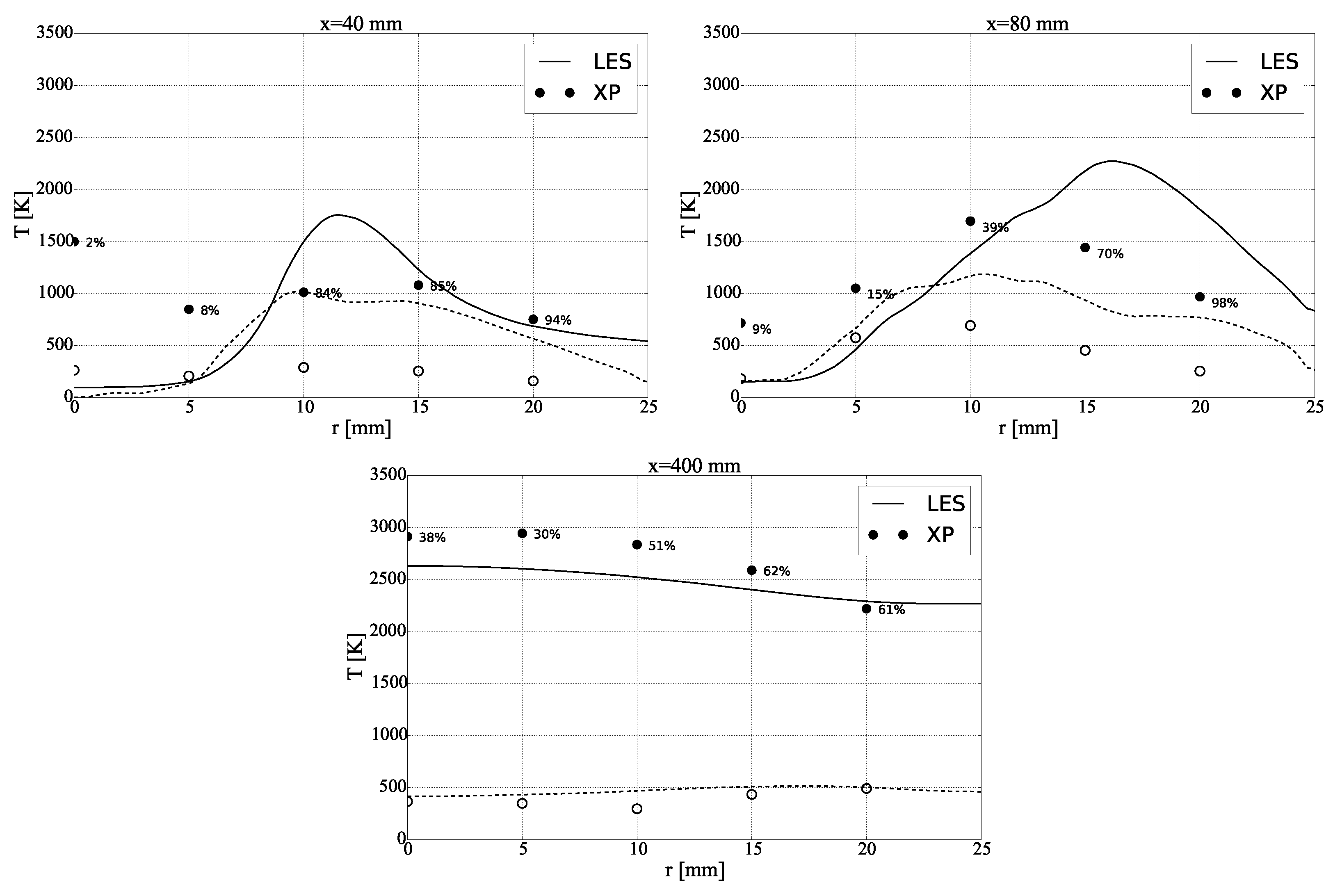
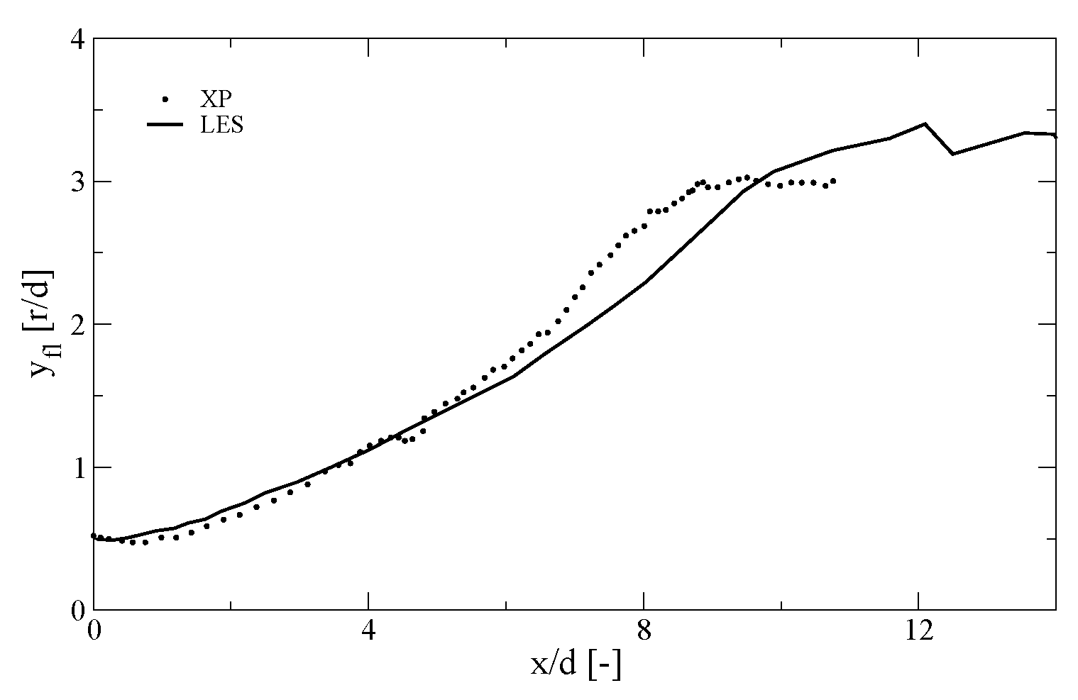
6.1. Case A1
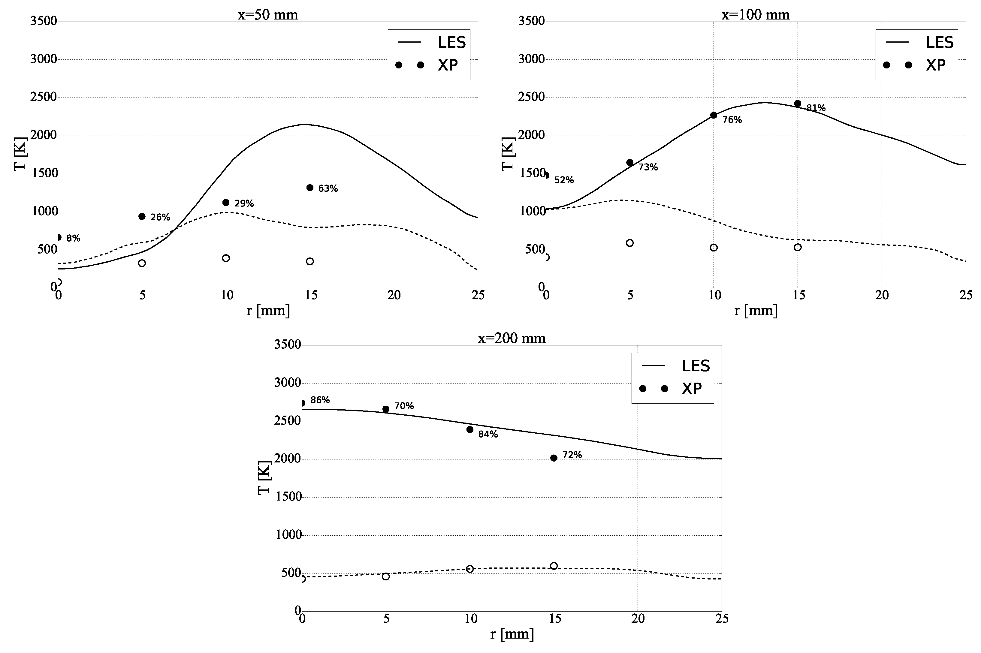
6.2. Cases A10
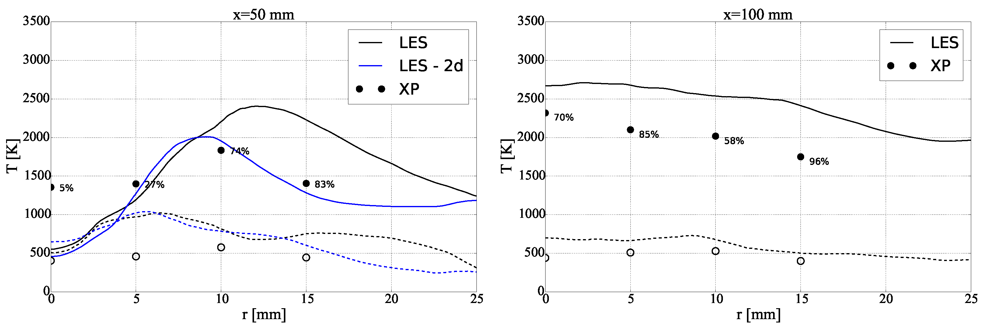
6.3. Case A30
7. Conclusions
Author Contributions
Funding
Institutional Review Board Statement
Informed Consent Statement
Data Availability Statement
Acknowledgments
Conflicts of Interest
Appendix A. Statistical Convergence


Appendix B. Comparison between Local and Homogeneous Grid Refinement for Case A30

References
- Candel, S.; Juniper, M.; Singla, G.; Scouflaire, P.; Rolon, C. Structure and Dynamics of Cryogenic Flames at Supercritical Pressure. Combust. Sci. Technol. 2006, 178, 161–192. [Google Scholar] [CrossRef]
- Oefelein, J. Mixing and combustion of cryogenic oxygen-hydrogen shear-coaxial jet flames at supercritical pressure. Combust. Sci. Technol. 2006, 178, 229–252. [Google Scholar] [CrossRef]
- Zong, N.; Yang, V. Cryogenic fluid jets and mixing layers in transcritical and supercritical environments. Combust. Sci. Technol. 2006, 178, 193–227. [Google Scholar] [CrossRef]
- Soave, G. Equilibrium constants from a modified Redlich-Kwong equation of state. Chem. Eng. Sci. 1977, 27, 1197–1203. [Google Scholar] [CrossRef]
- Schmitt, T.; Méry, Y.; Boileau, M.; Candel, S. Large-eddy simulation of oxygen/methane flames under transcritical conditions. Proc. Combust. Inst. 2011, 33, 1383–1390. [Google Scholar] [CrossRef]
- Zips, J.; Müller, H.; Pfitzner, M. Efficient thermo-chemistry tabulation for non-premixed combustion at high-pressure conditions. Flow Turbul. Combust. 2018, 101, 821–850. [Google Scholar] [CrossRef]
- Schmitt, T. Large-Eddy Simulations of the Mascotte Test Cases Operating at Supercritical Pressure. Flow Turbul. Combust. 2020, 105, 159–189. [Google Scholar] [CrossRef]
- Baer, M.; Nunziato, J. A two-phase mixture theory for the deflagration-to-detonation transition (DDT) in reactive granular materials. Int. J. Multiph. Flow 1986, 12, 861–889. [Google Scholar] [CrossRef]
- Saurel, R.; Abgrall, R. A multiphase Godunov Method for Compressible multifluid and multiphase flow. J. Comput. Phys. 1999, 150, 425–467. [Google Scholar] [CrossRef]
- Le Martelot, S.; Saurel, R.; Nkonga, B. Towards the direct numerical simulation of nucleate boiling flows. Int. J. Multiph. Flow 2014, 66, 62–78. [Google Scholar] [CrossRef]
- Matheis, J.; Hickel, S. Multi-component vapor-liquid equilibrium model for LES of high-pressure fuel injection and application to ECN Spray A. Int. J. Multiph. Flow 2018, 99, 294–311. [Google Scholar] [CrossRef]
- Traxinger, C.; Zips, J.; Pfitzner, M. Single-Phase Instability in Non-Premixed Flames Under Liquid Rocket Engine Relevant Conditions. J. Propuls. Power 2019, 35, 675–689. [Google Scholar] [CrossRef]
- Pelletier, M.; Schmitt, T.; Ducruix, S. A multifluid Taylor-Galerkin methodology for the simulation of compressible multicomponent separate two-phase flows from subcritical to supercritical states. Comput. Fluids 2020, 206, 104588. [Google Scholar] [CrossRef]
- Grisch, F.; Bouchardy, P.; Clauss, W. CARS thermometry in high pressure rocket combustors. Aerosp. Sci. Technol. 2003, 7, 317–330. [Google Scholar] [CrossRef]
- Vingert, L.; Habiballah, M.; Vuillermoz, P.; Zurbach, S. MASCOTTE, a test facility for cryogenic combustion research at high pressure. In Proceedings of the 51st International Astronautical Congress, Rio de Janeiro, Brazil, 2–6 October 2000. [Google Scholar]
- Habiballah, M.; Orain, M.; Grisch, F.; Vingert, L.; Gicquel, P. Experimental studies of high-pressure cryogenic flames on the Mascotte facility. Combust. Sci. Technol. 2006, 178, 101–128. [Google Scholar] [CrossRef]
- Kendrick, D.; Herding, G.; Scouflaire, P.; Rolon, C.; Candel, S. Effects of a recess on cryogenic flame stabilization. Combust. Flame 1999, 118, 327–339. [Google Scholar] [CrossRef]
- Herding, G.; Snyder, R.; Rolon, C.; Candel, S. Investigation of cryogenic propellant flames using computerized tomography of emission images. J. Propuls. Power 1998, 14, 146–151. [Google Scholar] [CrossRef]
- Poinsot, T.; Lele, S. Boundary conditions for direct simulations of compressible viscous flows. J. Comput. Phys. 1992, 101, 104–129. [Google Scholar] [CrossRef]
- Lee, L.L.; Starling, K.E.; Chung, T.H.; Ajlan, M. Generalized multiparameters corresponding state correlation for polyatomic, polar fluid transport properties. Ind. Chem. Eng. Res. 1988, 27, 671–679. [Google Scholar] [CrossRef]
- Nicoud, F.; Ducros, F. Subgrid-scale stress modelling based on the square of the velocity gradient. Flow, Turbul. Combust. 1999, 62, 183–200. [Google Scholar] [CrossRef]
- Poling, B.E.; Prausnitz, J.M.; O’Connel, J.P. The Properties of Gases and Liquids, 5th ed.; McGraw-Hill: New York, NY, USA, 2001. [Google Scholar]
- Pelletier, M. Diffuse Interface Models and Adapted Numerical Schemes for the Simulation of Subcritical to Supercritical Flows. PhD. Thesis, Université Paris-Saclay, Paris, France, 2019. [Google Scholar]
- Dapogny, C.; Dobrzynski, C.; Frey, P. Three-dimensional adaptive domain remeshing, implicit domain meshing, and applications to free and moving boundary problems. J. Comput. Phys. 2014, 262, 358–378. [Google Scholar] [CrossRef] [Green Version]
- Daviller, G.; Brebion, M.; Xavier, P.; Staffelbach, G.; Müller, J.D.; Poinsot, T. A Mesh Adaptation Strategy to Predict Pressure Losses in LES of Swirled Flows. Flow Turbul. Combust. 2017, 99, 93–118. [Google Scholar] [CrossRef]
- Schmitt, T. Assessment of Large-Eddy Simulation for the prediction of recessed inner-tube coaxial flames. Submitt. Ceas Space J. 2022. [Google Scholar]
- Le Touze, C.; Dorey, L.H.; Rutard, N.; Murrone, A. A compressible two-phase flow framework for Large Eddy Simulations of liquid-propellant rocket engines. Appl. Math. Model. 2020, 84, 265–286. [Google Scholar] [CrossRef]


| Case | [g/s] | [m/s] | P [bar] | We [-] | Experimental Data |
|---|---|---|---|---|---|
| A1 | 15 | 680 | 1 | 13,000 | CARS [14], OH*-emission [18] |
| A10 | 23.7 | 300 | 10 | 28,000 | CARS [14], OH*-emission [17,18] |
| A30 | 25.2 | 170 | 30 | 84,000 | CARS [14] |
| Mesh | Number of Refinement Iterations | Number of Nodes | CPU [kh] (for 10 ms) |
|---|---|---|---|
| M0 | 0 | 750,000 | 7.2 |
| M1 | 1 | 3,300,000 | 92 |
| M2 | 2 | 13,000,000 | 900 |
| Case | Mesh | |
|---|---|---|
| M0 | 36 ms | |
| A1 | M1 | 15 ms |
| M2 | 9 ms | |
| A10 | M0 | 68 ms |
| M1 | 33 ms | |
| M0 | 56 ms | |
| A30 | M1 | 39 ms |
| M2 | 9 ms |
Disclaimer/Publisher’s Note: The statements, opinions and data contained in all publications are solely those of the individual author(s) and contributor(s) and not of MDPI and/or the editor(s). MDPI and/or the editor(s) disclaim responsibility for any injury to people or property resulting from any ideas, methods, instructions or products referred to in the content. |
© 2023 by the authors. Licensee MDPI, Basel, Switzerland. This article is an open access article distributed under the terms and conditions of the Creative Commons Attribution (CC BY) license (https://creativecommons.org/licenses/by/4.0/).
Share and Cite
Schmitt, T.; Ducruix, S. Evaluation of Large-Eddy Simulation Coupled with an Homogeneous Equilibrium Model for the Prediction of Coaxial Cryogenic Flames under Subcritical Conditions. Aerospace 2023, 10, 98. https://doi.org/10.3390/aerospace10020098
Schmitt T, Ducruix S. Evaluation of Large-Eddy Simulation Coupled with an Homogeneous Equilibrium Model for the Prediction of Coaxial Cryogenic Flames under Subcritical Conditions. Aerospace. 2023; 10(2):98. https://doi.org/10.3390/aerospace10020098
Chicago/Turabian StyleSchmitt, Thomas, and Sébastien Ducruix. 2023. "Evaluation of Large-Eddy Simulation Coupled with an Homogeneous Equilibrium Model for the Prediction of Coaxial Cryogenic Flames under Subcritical Conditions" Aerospace 10, no. 2: 98. https://doi.org/10.3390/aerospace10020098