
E-Sail Optimal Trajectories to Heliostationary Points


Abstract
:1. Introduction
2. Mission Description and Mathematical Problem Statement
2.1. E-Sail Performance Requirements
2.2. Spacecraft Dynamics and Trajectory Optimization
3. Numerical Simulations and Parametric Analysis
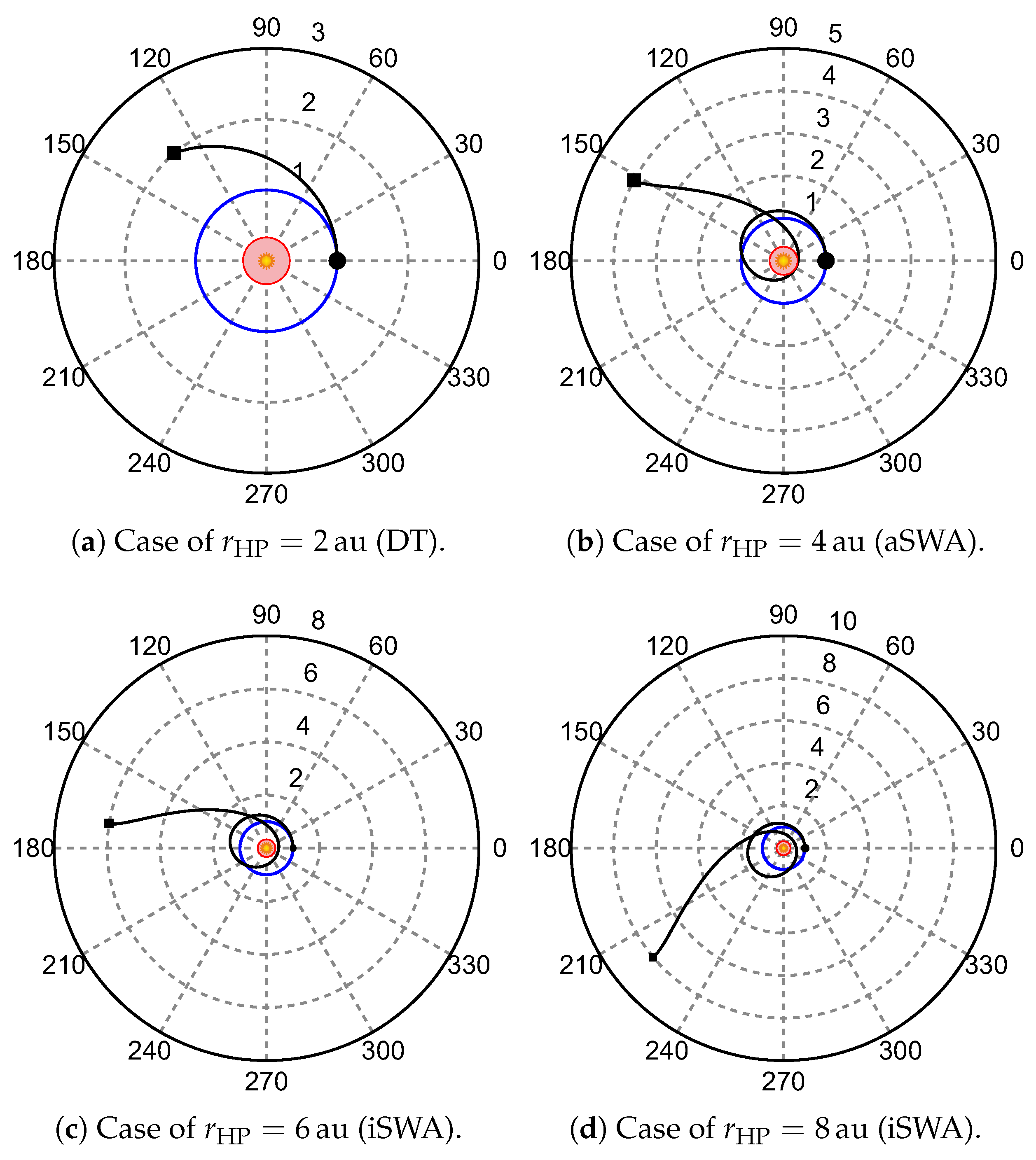
- Direct transfer (DT). During the optimal transfer, the Sun–spacecraft distance r continuously increases with time until the vehicle reaches the target HP, so that the perihelion distance of the optimal transfer coincides with the radius of the circular parking orbit; see Figure 5a.
- Solar wind assist with inactive perihelion constraint (iSWA). In this case, the minimum-time transfer trajectory contains a phase where the spacecraft approaches the Sun to increase its propulsive acceleration magnitude according to the thrust model of Equation (1). Paralleling the nomenclature used for a solar sail mission case [36], this behavior can be seen as a sort of solar wind assist (SWA) because of the thrust increase due to the variation of solar wind plasma density. The approaching phase ends when the spacecraft reaches a perihelion distance that, in this case, is greater than the minimum admissible value , so that the inequality constraint (14) is naturally satisfied (case of inactive constraint); see Figure 5b.
- Solar wind assist with active perihelion constraint (aSWA). This case is similar to the preceding one, with the only difference that the perihelion distance of the transfer trajectory is equal to as sketched in Figure 5c. In other terms, , and thus the constraint (14) on the solar distance becomes active at the perihelion.
3.1. Two-Dimensional Trajectory
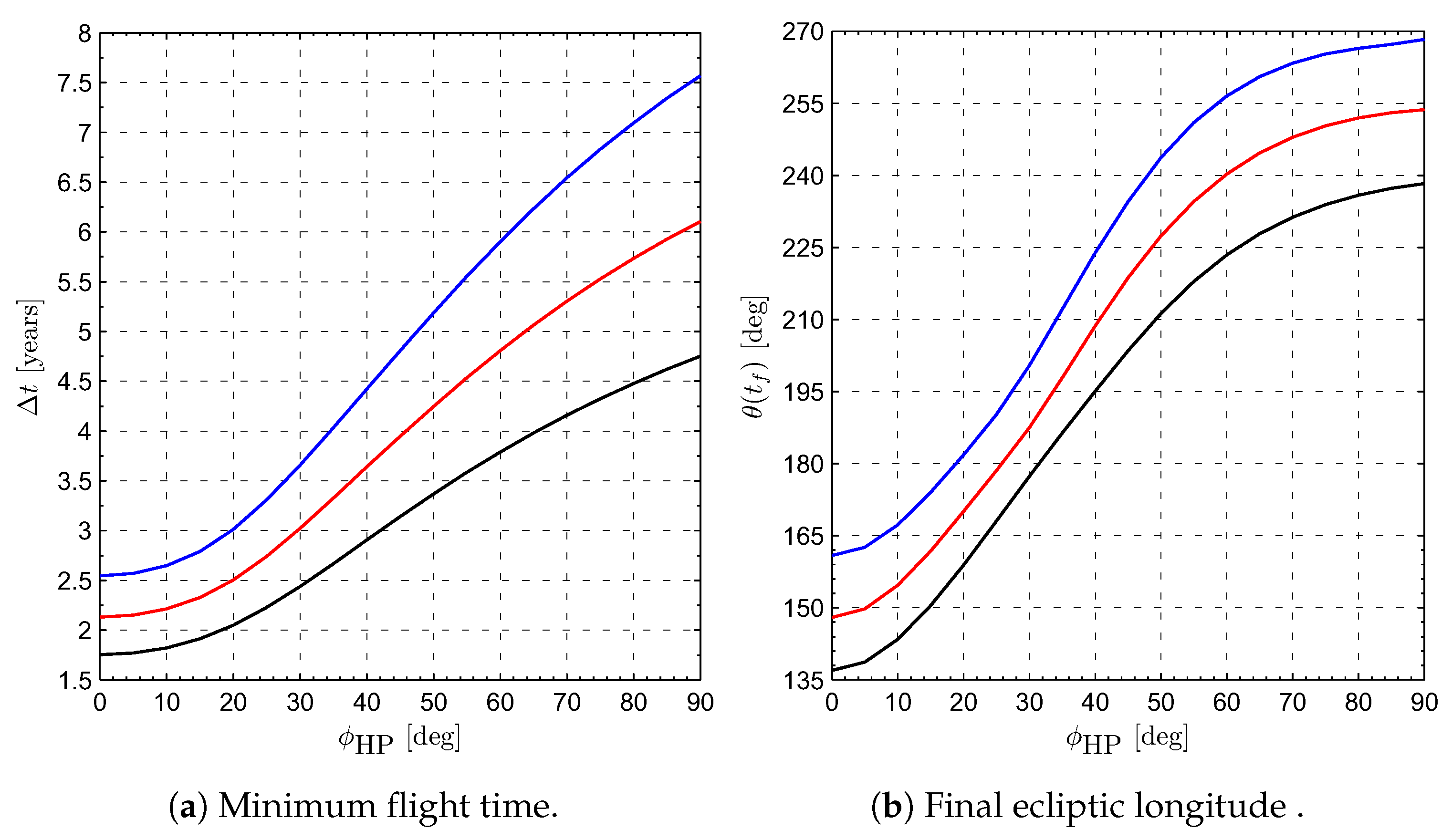
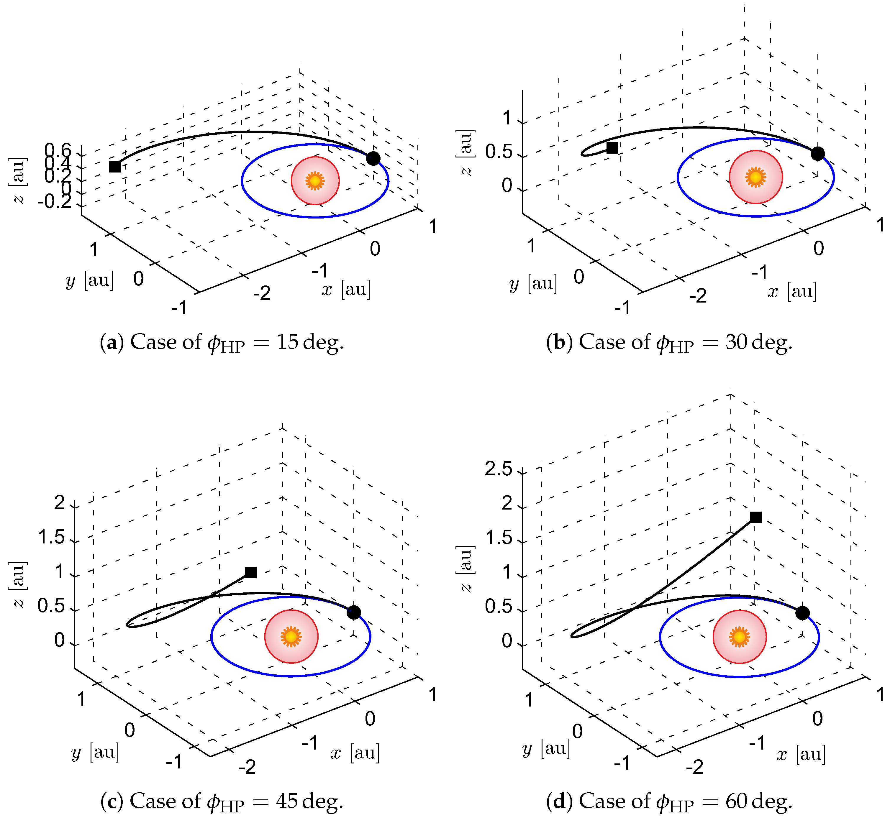
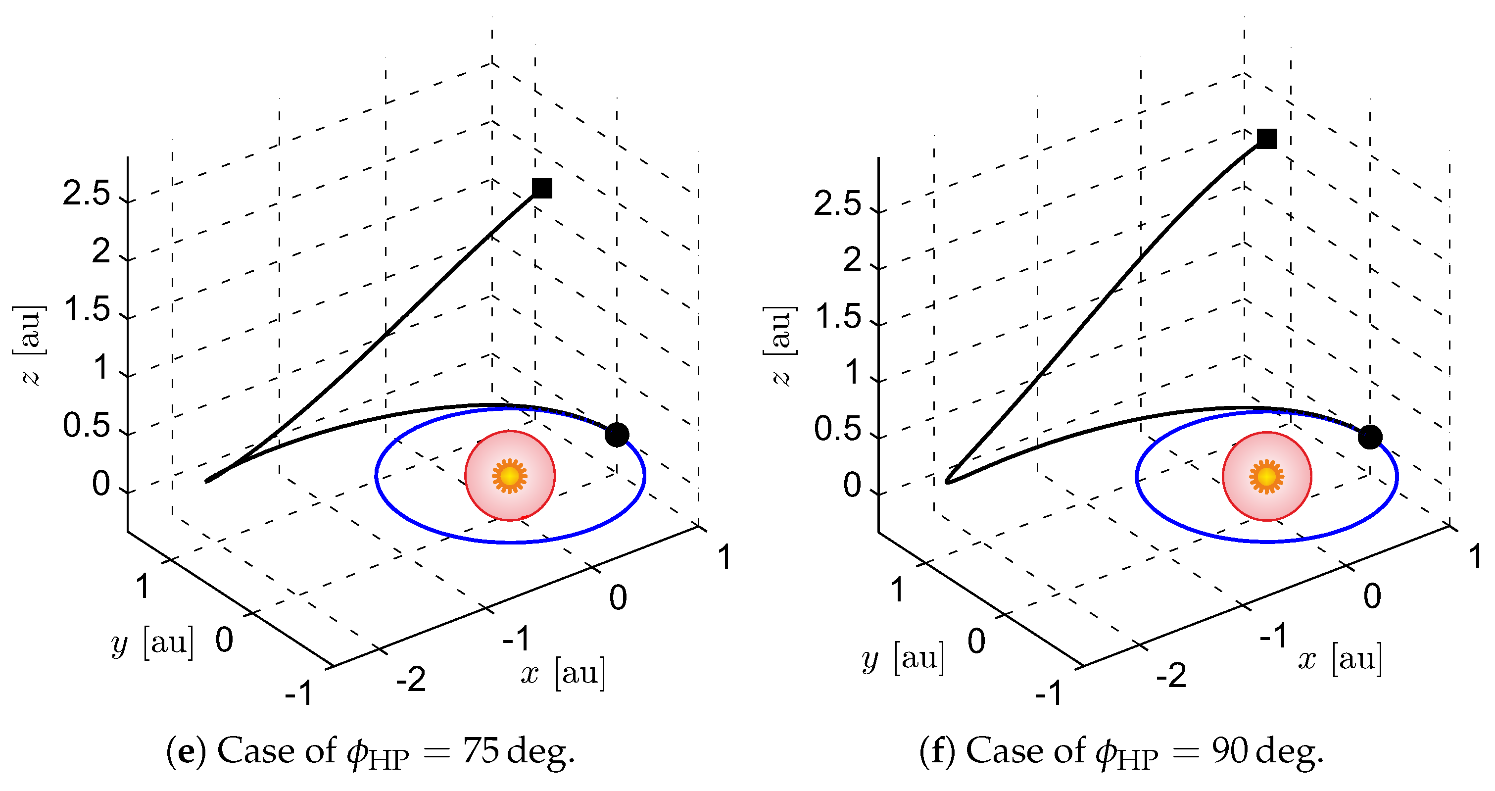
3.2. Three-Dimensional Scenario
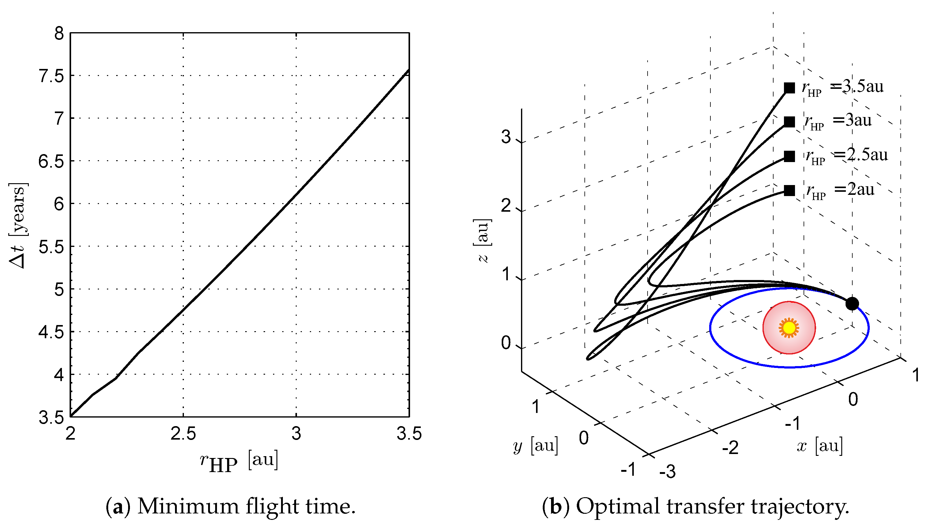
3.3. Mission Application
4. Conclusions
Author Contributions
Funding
Institutional Review Board Statement
Informed Consent Statement
Data Availability Statement
Conflicts of Interest
Abbreviations
| characteristic acceleration [mm/s] | |
| radial component of [mm/s] | |
| transverse component of [mm/s] | |
| azimuthal component of [mm/s] | |
| propulsive acceleration vector [mm/s] | |
| Hamiltonian function | |
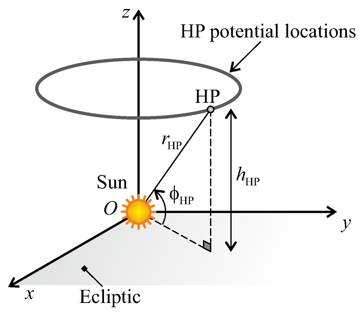
| h | distance from the ecliptic [au] |
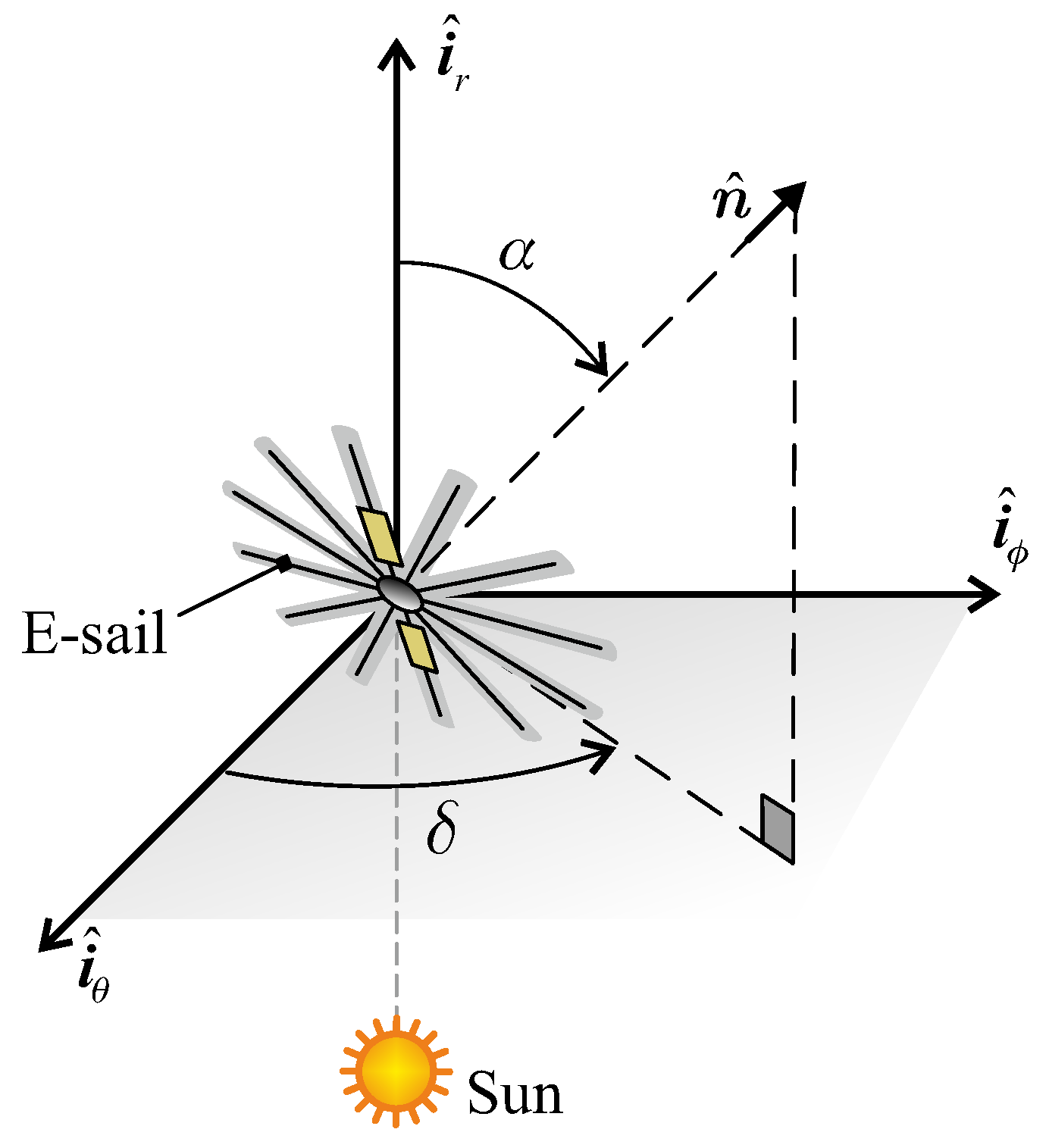
| radial unit vector | |
| transverse unit vector | |
| azimuthal unit vector | |
| J | performance index [days] |
| O | Sun’s center of mass |
| r | radial distance [au] |
| minimum perihelion radius [au] | |
| reference distance [] | |
| switching function | |
| t | time [days] |
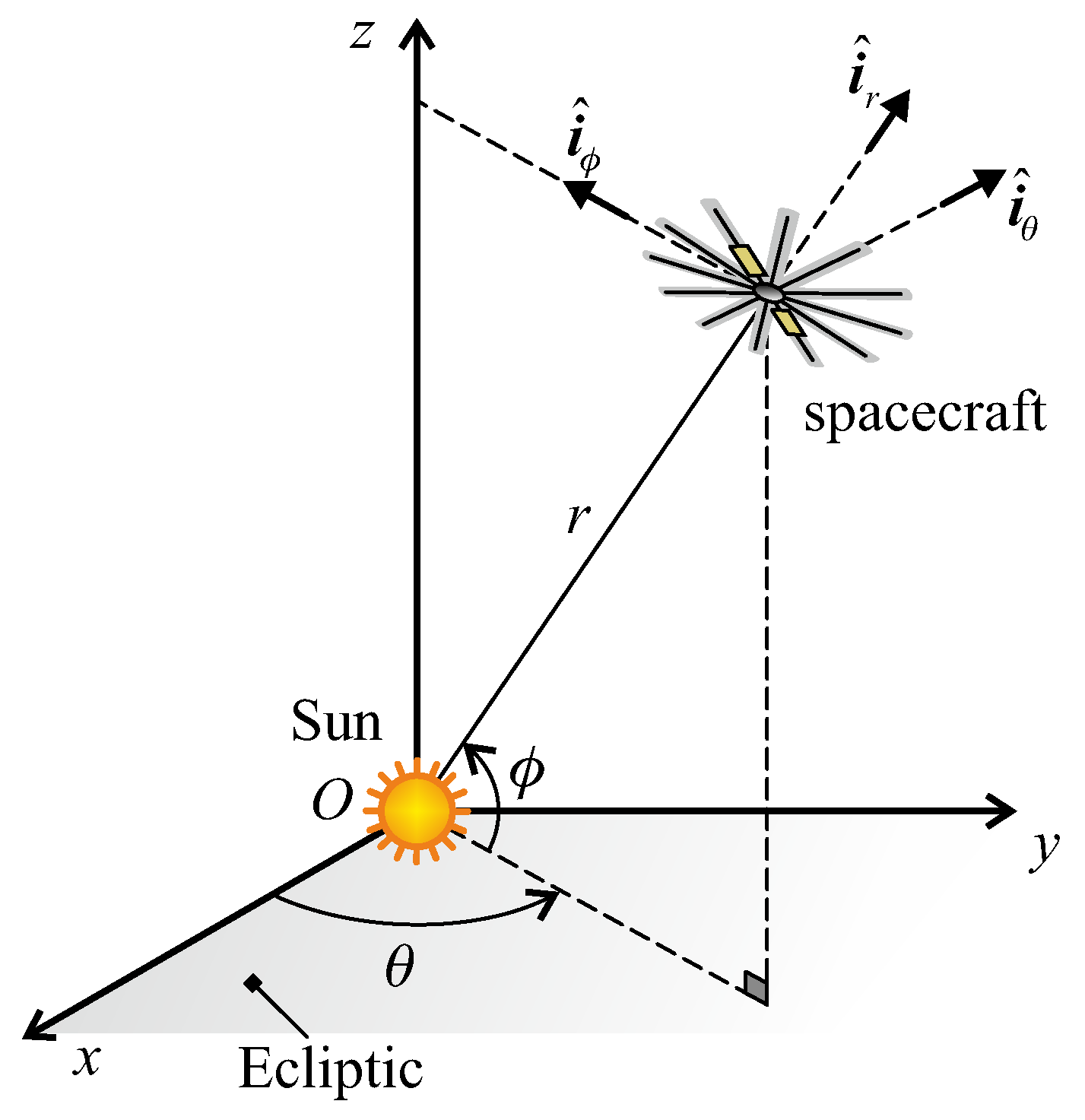
| spherical reference frame | |
| heliocentric-ecliptic reference frame | |
| radial component of the spacecraft velocity vector [km/s] | |
| transverse component of the spacecraft velocity vector [km/s] | |
| azimuthal component of the spacecraft velocity vector [km/s] | |
| sail cone angle [rad] | |
| flight time [days] | |
| sail clock angle [rad] | |
| ecliptic longitude [rad] | |
| variable adjoint to r | |
| variable adjoint to | |
| variable adjoint to | |
| variable adjoint to | |
| variable adjoint to | |
| variable adjoint to | |
| Sun’s gravitational parameter [km/s] | |
| dimensionless switching parameter | |
| ecliptic latitude [rad] | |
| Subscripts | |
| 0 | initial, parking orbit |
| f | final |
| HP | heliostationary point |
| p | perihelion |
| Superscripts | |
| · | derivative with respect to time |
| function of control variables |
Appendix A
References
- Forward, R.L. Statite—A spacecraft that does not orbit. J. Spacecr. Rocket. 1991, 28, 606–611. [Google Scholar] [CrossRef]
- Ceriotti, M.; Diedrich, B.L.; McInnes, C.R. Novel mission concepts for polar coverage: An overview of recent developments and possible future applications. Acta Astronaut. 2012, 80, 89–104. [Google Scholar] [CrossRef] [Green Version]
- Ceriotti, M.; Heiligers, J.; McInnes, C.R. Trajectory and Spacecraft Design for a Pole-Sitter Mission. J. Spacecr. Rocket. 2014, 51, 311–326. [Google Scholar] [CrossRef] [Green Version]
- McInnes, C.R. Inverse Solar Sail Trajectory Problem. J. Guid. Control. Dyn. 2003, 26, 369–371. [Google Scholar] [CrossRef]
- McKay, R.J.; Macdonald, M.; Biggs, J.; McInnes, C. Survey of Highly Non-Keplerian Orbits with Low-Thrust Propulsion. J. Guid. Control Dyn. 2011, 34, 645–666. [Google Scholar] [CrossRef] [Green Version]
- McInnes, C.R.; McDonald, A.J.C.; Simmons, J.F.L.; MacDonald, E.W. Solar sail parking in restricted three-body systems. J. Guid. Control Dyn. 1994, 17, 399–406. [Google Scholar] [CrossRef]
- Mengali, G.; Quarta, A.A. Optimal heliostationary missions of high-performance sailcraft. Acta Astronaut. 2007, 60, 676–683. [Google Scholar] [CrossRef]
- Quarta, A.A.; Mengali, G.; Niccolai, L. Solar Sail Optimal Transfer Between Heliostationary Points. J. Guid. Control Dyn. 2020, 43, 1935–1942. [Google Scholar] [CrossRef]
- Fu, B.; Sperber, E.; Eke, F. Solar sail technology—A state of the art review. Prog. Aerosp. Sci. 2016, 86, 1–19. [Google Scholar] [CrossRef]
- Gong, S.; Macdonald, M. Review on solar sail technology. Astrodynamics 2019, 3, 93–125. [Google Scholar] [CrossRef]
- Dachwald, B.; Mengali, G.; Quarta, A.A.; Macdonald, M. Parametric model and optimal control of solar sails with optical degradation. J. Guid. Control Dyn. 2006, 29, 1170–1178. [Google Scholar] [CrossRef]
- Davoyan, A.R.; Munday, J.N.; Tabiryan, N.; Swartzlander, G.A.; Johnson, L. Photonic materials for interstellar solar sailing. Optica 2021, 8, 722–734. [Google Scholar] [CrossRef]
- Bruno, C.; Accettura, A.G.; Seboldt, W.; Dachwald, B. Advanced Propulsion Systems and Technologies, Today to 2020; American Institute of Aeronautics and Astronautics: Reston, VA, USA, 2008; Chapter 1, 16; pp. 1–18;427–452 . [Google Scholar] [CrossRef]
- Vilela Salgado, M.C.; Neyra Belderrain, M.C.; Campos Devezas, T. Space Propulsion: A Survey Study About Current and Future Technologies. J. Aerosp. Technol. Manag. 2018, 10, 1–23. [Google Scholar] [CrossRef]
- Janhunen, P.; Toivanen, P.K.; Polkko, J.; Merikallio, S.; Salminen, P.; Haeggström, E.; Seppänen, H.; Kurppa, R.; Ukkonen, J.; Kiprich, S.; et al. Electric solar wind sail: Toward test missions. Rev. Sci. Instrum. 2010, 81, 111301-1–11301-11. [Google Scholar] [CrossRef] [PubMed]
- Janhunen, P. Electric sail for spacecraft propulsion. J. Propuls. Power 2004, 20, 763–764. [Google Scholar] [CrossRef]
- Janhunen, P.; Sandroos, A. Simulation study of solar wind push on a charged wire: Basis of solar wind electric sail propulsion. Ann. Geophys. 2007, 25, 755–767. [Google Scholar] [CrossRef] [Green Version]
- Bassetto, M.; Niccolai, L.; Quarta, A.A.; Mengali, G. A comprehensive review of Electric Solar Wind Sail concept and its applications. Prog. Aerosp. Sci. 2022, 128, 100768. [Google Scholar] [CrossRef]
- Janhunen, P.; Toivanen, P.; Envall, J.; Slavinskis, A. Using charged tether Coulomb drag: E-sail and plasma brake. In Proceedings of the Fifth International Conference on Tethers in Space, Ann Arbor, MI, USA, 24–26 May 2016. [Google Scholar]
- Toivanen, P.K.; Janhunen, P. Thrust vectoring of an electric solar wind sail with a realistic sail shape. Acta Astronaut. 2017, 131, 145–151. [Google Scholar] [CrossRef] [Green Version]
- Huo, M.Y.; Mengali, G.; Quarta, A.A. Electric sail thrust model from a geometrical perspective. J. Guid. Control Dyn. 2018, 41, 735–741. [Google Scholar] [CrossRef]
- Bassetto, M.; Mengali, G.; Quarta, A.A. Stability and control of spinning E-sail in heliostationary orbit. J. Guid. Control Dyn. 2019, 42, 425–431. [Google Scholar] [CrossRef]
- Bate, R.R.; Mueller, D.D.; White, J.E. Fundamentals of Astrodynamics; Dover Publications: New York, NY, USA, 1971; Chapter 2; pp. 53–55. [Google Scholar]
- Merikallio, S.; Janhunen, P. The electric solar wind sail (E-sail): Propulsion innovation for solar system travel. Bridge 2018, 48, 28–32. [Google Scholar]
- Wiegmann, B.M. Conceptual Design of an Electric Sail Technology Demonstration Mission Spacecraft. In Proceedings of the 40th Annual AAS Rocky Mountain Section Guidance and Control Conference, Breckenridge, CO, USA, 2–8 February 2017. [Google Scholar]
- Mengali, G.; Quarta, A.A.; Janhunen, P. Electric sail performance analysis. J. Spacecr. Rocket. 2008, 45, 122–129. [Google Scholar] [CrossRef]
- Quarta, A.A.; Mengali, G.; Bassetto, M.; Niccolai, L. Optimal circle-to-ellipse orbit transfer for Sun-facing E-sail. Aerospace 2022, 9, 671. [Google Scholar] [CrossRef]
- Niccolai, L.; Quarta, A.A.; Mengali, G.; Bassetto, M. Trajectory analysis of a zero-pitch angle E-sail with homotopy perturbation technique. J. Guid. Control Dyn. 2023; in press. [Google Scholar] [CrossRef]
- Mengali, G.; Quarta, A.A.; Aliasi, G. A graphical approach to electric sail mission design with radial thrust. Acta Astronaut. 2013, 82, 197–208. [Google Scholar] [CrossRef]
- Quarta, A.A.; Mengali, G. Analysis of electric sail heliocentric motion under radial thrust. J. Guid. Control Dyn. 2016, 39, 1431–1435. [Google Scholar] [CrossRef]
- Janhunen, P.; Quarta, A.A.; Mengali, G. Electric solar wind sail mass budget model. Geosci. Instrum. Methods Data Syst. 2013, 2, 85–95. [Google Scholar] [CrossRef] [Green Version]
- Wie, B. Thrust Vector Control Analysis and Design for Solar-Sail Spacecraft. J. Spacecr. Rocket. 2007, 44, 545–557. [Google Scholar] [CrossRef]
- Mengali, G.; Quarta, A.A. Non-Keplerian orbits for electric sails. Celest. Mech. Dyn. Astron. 2009, 105, 179–195. [Google Scholar] [CrossRef]
- Quarta, A.A.; Mengali, G. Electric sail mission analysis for outer solar system exploration. J. Guid. Control Dyn. 2010, 33, 740–755. [Google Scholar] [CrossRef]
- Bryson, A.E.J.; Ho, Y.C. Applied Optimal Control; Taylor & Francis Group: New York, NY, USA, 1975. [Google Scholar]
- Leipold, M.; Wagner, O. ‘Solar photonic assist’ trajectory design for solar sail missions to the outer solar system and beyond. In Proceedings of the AAS/GSFC International Symposium on Flight Dynamics, Greenbelt, MD, USA, 11–15 May 1998. [Google Scholar]


Disclaimer/Publisher’s Note: The statements, opinions and data contained in all publications are solely those of the individual author(s) and contributor(s) and not of MDPI and/or the editor(s). MDPI and/or the editor(s) disclaim responsibility for any injury to people or property resulting from any ideas, methods, instructions or products referred to in the content. |
© 2023 by the authors. Licensee MDPI, Basel, Switzerland. This article is an open access article distributed under the terms and conditions of the Creative Commons Attribution (CC BY) license (https://creativecommons.org/licenses/by/4.0/).
Share and Cite
Quarta, A.A.; Mengali, G. E-Sail Optimal Trajectories to Heliostationary Points. Aerospace 2023, 10, 194. https://doi.org/10.3390/aerospace10020194
Quarta AA, Mengali G. E-Sail Optimal Trajectories to Heliostationary Points. Aerospace. 2023; 10(2):194. https://doi.org/10.3390/aerospace10020194
Chicago/Turabian StyleQuarta, Alessandro A., and Giovanni Mengali. 2023. "E-Sail Optimal Trajectories to Heliostationary Points" Aerospace 10, no. 2: 194. https://doi.org/10.3390/aerospace10020194