E-Sail Option for Plunging a Spacecraft into the Sun’s Atmosphere

Abstract

A close observation of the near-Sun region, with in situ measurements, requires that a scientific probe be placed in a heliocentric orbit with a perihelion distance on the order of a few solar radii only. This is the solution adopted by the Parker Solar Probe (PSP), whose mission design uses a very complex transfer trajectory with seven Venus gravity assists to reach a perihelion radius of roughly $9.9$ solar radii in about seven years. This paper aims to discuss the capability of an Electric Solar-Wind Sail (E-sail), i.e., a propellantless propulsion system that exploits the solar wind as a deep-space thrust source using a grid of long and artificially charged tethers, to drive a scientific probe toward a heliocentric orbit with characteristics similar to that considered during the initial design of the PSP mission. The two-dimensional trajectory analysis of an E-sail-based spacecraft is performed in an optimal framework, by considering the physical constraints induced by the thermal loads acting on the propellantless propulsion system when the spacecraft approaches the inner Sun regions. This means that, during the transfer trajectory, the E-sail-based spacecraft must avoid a spherical region around the Sun whose radius depends on the mechanical characteristics of the charged tethers. The paper shows that feasible solutions, in terms of optimal transfer trajectories, are possible even when a medium-performance E-sail is considered in the spacecraft design. In that context, the obtained trajectory can drive a scientific probe on the target (high elliptic) orbit in less than two years, without the use of any intermediate flyby maneuver.

1. Introduction

The study of the Sun and its interactions with the terrestrial planets is crucial for understanding the physical phenomena and the local properties of the near-Earth space environment. For example, a close observation of the near-Sun regions, with in situ measurements, is a fundamental step in the collection of necessary data and the elaboration of a reliable model of the solar magnetic field with an accurate solar-wind description. In this regard, the recent success of NASA’s historic Parker Solar Probe (PSP) mission, which is a milestone in the more ambitious NASA Living with a Star program [1,2], demonstrates the importance of the local observation of the near-Sun space. The PSP mission was conceived to investigate the Sun’s corona from inside and obtain accurate information on the upper solar atmosphere, the occurrence of solar flares and coronal mass ejections, the composition, structure and properties of the solar wind [3], and the influence of solar activity on space weather and the terrestrial environment [4,5].

To meet these scientific objectives, the probe must fly close to the Sun, i.e., its heliocentric orbit must have a very small perihelion distance, in the order of a few solar radii. This requirement makes such a type of scientific mission really a challenging problem due to the velocity change and the launch energy it requires. Not surprisingly, the PSP scenario called for several mission proposals and several changes and new designs [6]. The final trajectory, which is currently flown by the probe since 2018 (when it was launched), has an involved shape [7] and uses seven Venus flybys and approximately seven years to gradually decrease the probe perihelion distance to about $9.9R_{\odot }$ or $0.046\mathrm{au}$, where $R_{\odot }$ is the reference value of the solar radius. The complexity of the PSP trajectory is the result of several design constraints [7], including the total mission costs (less than $750 M), the lack of any source of nuclear power, the requirement of three solar passes with perihelion distance smaller than $10R_{\odot }$, and a total mission flight time less than $10\mathrm{years}$. In particular, the exclusion of radioisotope thermoelectric generators imposed a full mission reappraisal, discarding the idea of using a gravity assist from Jupiter, as planned in early mission design [7]. The renunciation of the Jupiter swingby called for multiple flybys with Venus to reduce the probe velocity enough and allow the spacecraft to approach the Sun at the desired (very close) distance.

This paper aims to analyze, with a simplified two-dimensional approach, a different solution to the transfer problem of a scientific probe to a high elliptic orbit with a very low perihelion radius, by looking for a new trajectory that, while satisfying the main constraints of the original concept behind the PSP mission scenario, can avoid the need for planetary flybys. The proposed approach uses a spacecraft propelled by an Electric Solar-Wind Sail (E-sail), i.e., an innovative propellantless propulsion concept able to produce a deep-space thrust by exploiting the electrostatic interaction between solar-wind ions and a charged tether grid [8,9]. Since an E-sail operates without any propellant stored onboard, it represents a very interesting option for propellantless missions requiring a continuous (and steerable) propulsive acceleration, and, indeed, it has been proposed for different advanced mission scenarios, such as, for example, the reaching of displaced non-Keplerian orbits [10], Solar System escape [11,12], or the maintenance of artificial equilibrium points in the Sun–Earth gravitational field [13]. Another potential application for an E-sail is a mission aimed at reaching high heliolatitudes with a perihelion near the Sun. From that position, it would be possible, through in situ measurements, to analyze electric current structures [14], whose sources are not yet sufficiently studied. Finally, an E-sail propulsion system may also represent an interesting means to insert a scientific probe into a high elliptic orbit with a perihelion radius inside the Sun’s upper atmosphere, as is undertaken by the PSP mission, but using a less involved interplanetary trajectory. Moreover, the E-sail can reach high heliolatitudes with perihelion near the Sun, in order to analyze (through in situ measurements) electric current structures [14], whose sources are not yet sufficiently studied. In the context of a two-dimensional scenario, the transfer trajectory analysis is performed in an optimal framework, by considering the physical constraints induced by the thermal loads acting on the E-sail when it approaches the Sun [15]. In practice, during the transfer, the spacecraft distance from the Sun cannot decrease below a minimum admissible value. Such a mission (path) constraint makes the interplanetary trajectory design a difficult problem to solve, because the E-sail minimum allowable distance from the Sun is one order of magnitude greater than the perihelion radius of the target, high elliptic, orbit.

2. Mission Description and Mathematical Preliminaries

Consider a two-dimensional heliocentric mission scenario, in which a spacecraft initially traces an Ecliptic circular orbit of radius $r_{\oplus }\triangleq 1\mathrm{au}$. This situation is consistent with a simplified case where the spacecraft uses a parabolic escape trajectory relative to the Earth, and the eccentricity of the planet’s orbit is neglected. The interplanetary mission requires the scientific probe to be transferred to a coplanar elliptic orbit, with a perihelion distance $r_{p_t}$ close to the star to make in situ observations of the Sun’s upper atmosphere. To that end, the scientific probe must be designed to correctly operate under extreme conditions, such as those expected in the near-Sun environment, i.e., in presence of large temperature fluctuations and strong magnetic fields. In addition, the aphelion radius $r_{a_t}$ of the target orbit should not be too far from the Sun [7] to allow the solar panels to supply the necessary power to onboard systems without the need for resorting to radioisotope thermoelectric generators. Recalling the main design parameters of NASA’s PSP and using the data reported by Guo [7], it is assumed that the target orbit of the scientific probe has the following characteristics

$$r_{p_t}=10R_{\odot }\simeq 0.0465\mathrm{au},r_{a_t}=1\mathrm{au}$$

(1)

that is, the semimajor axis and eccentricity of the heliocentric target orbit are, respectively,

$$a_t=0.523\mathrm{au},e_t=0.911$$

(2)

These data correspond to a highly eccentric orbit with an orbital period of about $138\mathrm{days}$ and a very low perihelion radius. Please note that the nominal final orbit of the PSP has a perihelion radius equal to $9.9R_{\odot }$, an aphelion radius of about $0.73\mathrm{au}$ (the aphelion point is near the heliocentric orbit of Venus), and an orbital period of about $88\mathrm{days}$.

The spacecraft propulsion system is an E-sail, which is used to transfer the scientific probe from the parking circular orbit to the target orbit with elements $\{a_t,e_t\}$ defined in Equation (2). Since the E-sail charged tethers cannot operate near the Sun, due to the thermal loads coming from the star, the spacecraft can be ideally thought of as divided into two main macro-components, i.e., the scientific probe and the E-sail-based module, which is jettisoned once the scientific probe is inserted into the target, high elliptic, orbit. In practice, the conceptual design of the E-sail propulsion system [9] prevents the propellantless thruster from operating below a minimum solar distance $r_m$, which depends on the charged tether characteristics. 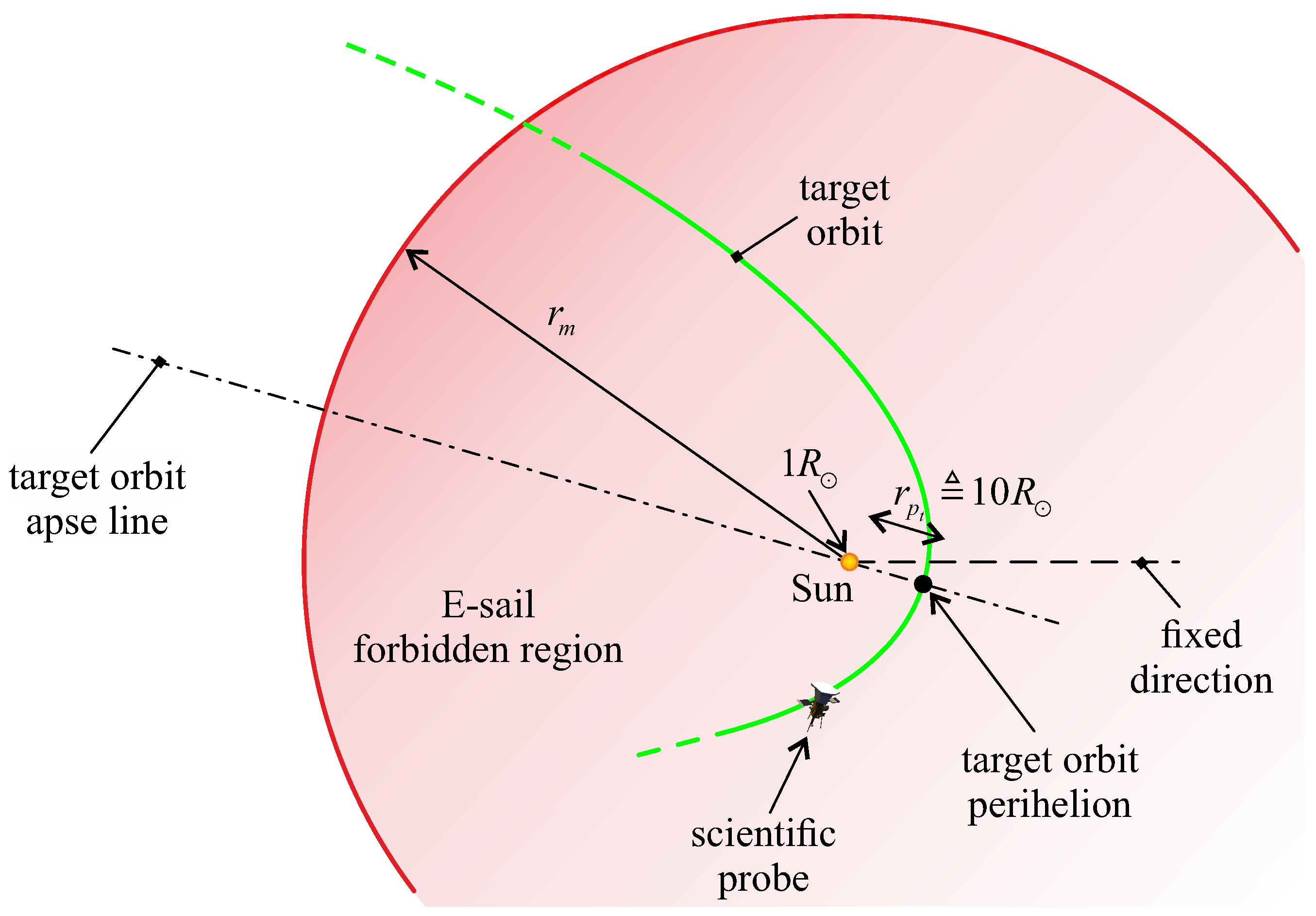For example, in case of copper tethers, the minimum solar distance is $r_m=0.33\mathrm{au}$, while aluminum tethers impose the thruster to operate at a higher distance, i.e., $r_m=0.5\mathrm{au}$ from the Sun [15]. In the rest of the paper, a copper tether case is assumed, so that the constraint on the Sun–spacecraft distance during the transfer is

$$r\ge r_m\triangleq 0.33\mathrm{au}$$

(3)

The latter inequality corresponds to a path constraint to be enforced along the transfer trajectory. Note that, in a two-dimensional mission scenario, Equation (3) describes a forbidden circular region centered at the Sun, which partially contains the target highly elliptic orbit, as sketched in Figure 1. This particular mixture of orbit shape and path constraint makes the transfer trajectory design a difficult task to solve, as discussed below.

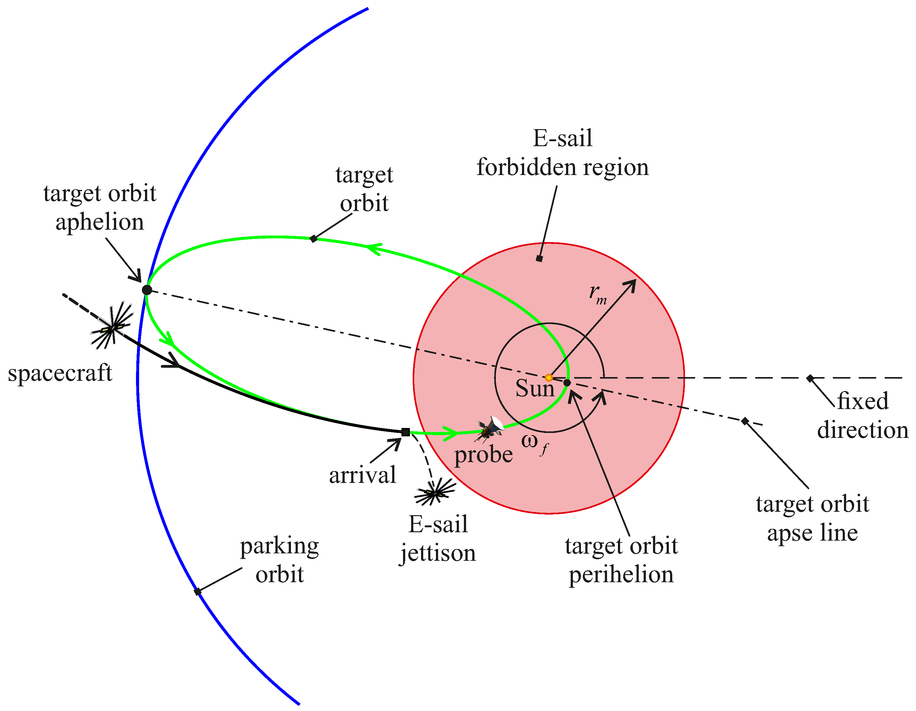
Figure 1 also shows the target orbit apse line and a fixed direction in the Ecliptic, which is useful for detecting the spacecraft’s azimuthal position during the transfer. Let ${\omega }_f\in [0,360]\mathrm{deg}$ be the argument of periapsis of the target orbit, calculated for the fixed direction, as shown in Figure 2. The apse line orientation is left free, i.e., ${\omega }_f$ is unconstrained and is an output of the optimization process used to design the spacecraft transfer trajectory, as discussed later in the paper.

2.1. Spacecraft Dynamics

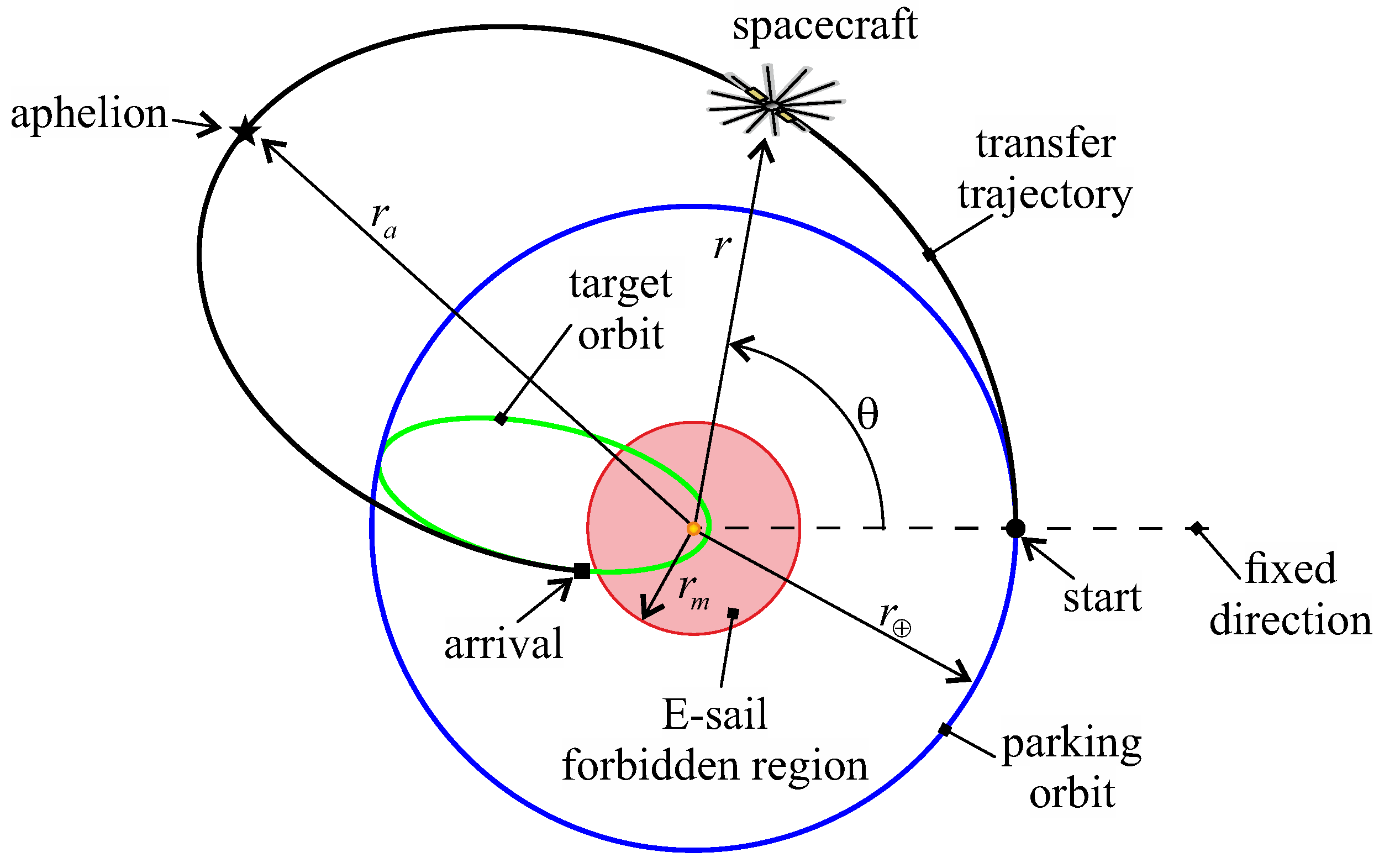
During the interplanetary transfer, the spacecraft dynamics may be conveniently described with the aid of a polar reference frame $\mathcal{T}(O;r,\theta )$, the origin of which (point O) coincides with the Sun’s center-of-mass, and $\theta$ is the polar angle measured counterclockwise from the fixed direction. The latter is assumed to coincide with the Sun–spacecraft line at the initial time $t=t_0\triangleq 0$; see Figure 3.

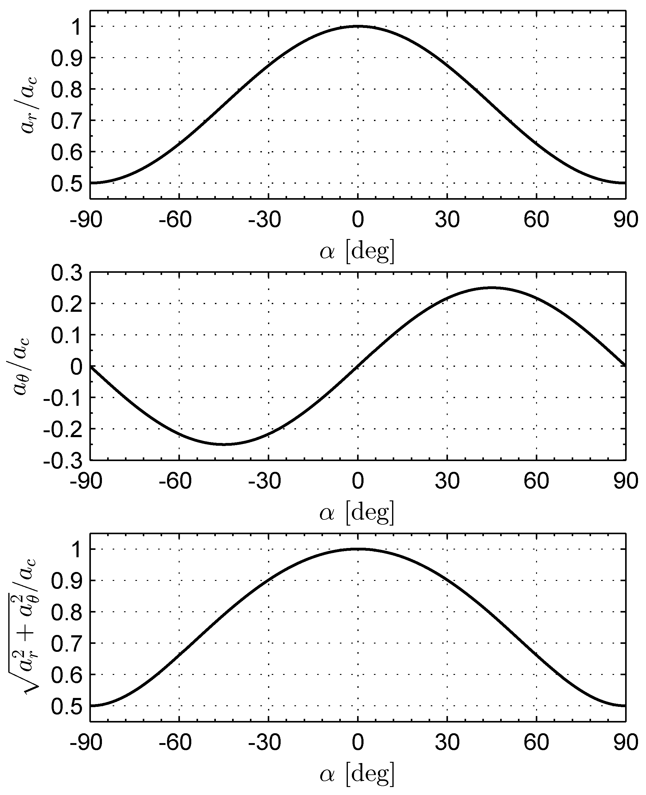
The E-sail-induced propulsive acceleration is described by the thrust model proposed by Huo et al. [16], according to which the radial ($a_r$) and transverse ($a_{\theta }$) components of the propulsive acceleration vector are

$$\begin{array}{cc}\hfill a_r& =\tau \frac{a_c}{2}\left(\frac{r_{\oplus }}{r}\right)\left(1+cos{\alpha }^2\right)\hfill \end{array}$$

(4)

$$\begin{array}{cc}\hfill a_{\theta }& =\tau \frac{a_c}{2}\left(\frac{r_{\oplus }}{r}\right)\left(cos\alpha sin\alpha \right)\hfill \end{array}$$

(5)

where $\tau \in \{0,1\}$ is a switching dimensionless parameter, which models the E-sail electron gun operating mode [17], either on (when $\tau =1$) or off (i.e., $\tau =0$), $\alpha \in [-90,90]\mathrm{deg}$ is the pitch angle, defined as the angle between the radial line and the normal to the sail nominal plane in the direction opposite to the Sun, and $a_c$ is the characteristic acceleration, i.e., the maximum propulsive acceleration magnitude at a solar distance equal to one astronomical unit. Here, the nominal plane is defined as the plane that ideally contains the E-sail charged tethers. The variations of the two components $\{a_r,a_{\theta }\}$ and that of the acceleration magnitude $\sqrt{a_r^2+a_{\theta }^2}$ with the sail pitch angle are reported (in dimensionless form) in Figure 4 when $\tau =1$ and $r=r_{\oplus }$.

Using the expressions taken from Equations (4) and (5), the spacecraft equations of motion in the polar reference frame $\mathcal{T}$ are

$$\begin{array}{cc}\hfill \dot{r}& =u\hfill \end{array}$$

(6)

$$\begin{array}{cc}\hfill \dot{\theta }& =\frac{v}{r}\hfill \end{array}$$

(7)

$$\begin{array}{cc}\hfill \dot{u}& =\frac{{\mu }_{\odot }}{r^2}+\frac{v^2}{r}+\tau \frac{a_c}{2}\left(\frac{r_{\oplus }}{r}\right)\left(1+cos{\alpha }^2\right)\hfill \end{array}$$

(8)

$$\begin{array}{cc}\hfill \dot{v}& =-\frac{uv}{r}+\tau \frac{a_c}{2}\left(\frac{r_{\oplus }}{r}\right)\left(cos\alpha sin\alpha \right)\hfill \end{array}$$

(9)

where u (or v) is the radial (or transverse) component of the spacecraft inertial velocity, and ${\mu }_{\odot }$ is the Sun’s gravitational parameter. The differential system (6)–(9) is completed by four initial conditions. Since the spacecraft’s initial trajectory is a circular orbit of radius $r_{\oplus }$, the initial conditions are

$$r\left(t_0\right)=r_{\oplus },\theta \left(t_0\right)=0,u\left(t_0\right)=0,v\left(t_0\right)=\sqrt{\frac{{\mu }_{\odot }}{r_{\oplus }}}$$

(10)

where the initial polar angle is set equal to zero as it is measured from the fixed direction; see Figure 3.

2.2. Remarks on Trajectory Optimization

For a given characteristic acceleration $a_c$, the time variation of the sail pitch angle has been obtained by minimizing the flight time $\Delta t=t_f-t_0\equiv t_f$ required to transfer the spacecraft from the circular parking orbit of radius $r_{\oplus }$ to the (coplanar) elliptic orbit of elements $\{a_t,e_t\}$ given by Equation (2). The terminal conditions of Equation (2) can be translated into two equivalent constraints involving the final (i.e., calculated at the unknown time $t_f)$ values of the spacecraft states $\{r,u,v\}$, viz.

$$\begin{array}{cc}\hfill & \frac{u{\left(t_f\right)}^2+v{\left(t_f\right)}^2}{2}-\frac{{\mu }_{\odot }}{r\left(t_f\right)}=-\frac{{\mu }_{\odot }}{2a_t}\hfill \end{array}$$

(11)

$$\begin{array}{cc}\hfill & r\left(t_f\right)v\left(t_f\right)=\sqrt{{\mu }_{\odot }{a}_t\left(1-e_t^2\right)}\hfill \end{array}$$

(12)

Please note that the right-hand side term in Equation (11) (or in Equation (12)) coincides with the specific mechanical energy (or the specific angular momentum magnitude) of the target orbit. As a result, the problem amounts to looking for the transfer trajectory that minimizes the time necessary to move the dynamical system from the initial state (10) to the state defined by Equations (11) and (12), while enforcing the path constraint on the radial distance given by Equation (3). This problem has been solved with an indirect approach [18], paralleling the procedure described in Ref. [15]. The Hamiltonian function is

$$\mathcal{H}\triangleq {\lambda }_r\dot{r}+{\lambda }_{\theta }\dot{\theta }+{\lambda }_u\dot{u}+{\lambda }_v\dot{v}$$

(13)

where $\{{\lambda }_r,{\lambda }_{\theta },{\lambda }_u,{\lambda }_v\}$ are the variables adjoint to $\{r,\theta ,u,v\}$, respectively. The time derivative of a generic adjoint variable is obtained from the Euler-Lagrange equations

$${\dot{\lambda }}_i=-\frac{\partial \mathcal{H}}{\partial i}\mathrm{where}i=\{r,\theta ,u,v\}$$

(14)

the explicit expression of which is here omitted for the sake of brevity. The additional boundary constraints are obtained from the transversality condition [18], i.e.,

$$\begin{array}{cc}\hfill \mathcal{H}\left(t_f\right)& =1\hfill \end{array}$$

(15)

$$\begin{array}{cc}\hfill {\lambda }_{\theta }\left(t_f\right)& =0\hfill \end{array}$$

(16)

$$\begin{array}{cc}\hfill {\lambda }_u\left(t_f\right)\left[{\mu }_{\odot }-r\left(t_f\right)v{\left(t_f\right)}^2\right]& =r\left(t_f\right)u\left(t_f\right)\left[{\lambda }_r\left(t_f\right)r\left(t_f\right)-{\lambda }_v\left(t_f\right)v\left(t_f\right)\right]\hfill \end{array}$$

(17)

Finally, the optimal control law, i.e., the variation of the sail pitch angle $\alpha$ and that of the switching parameter $\tau$ as a function of the adjoint variables is derived from the general results of Ref. [16].

The open-time unconstrained transfer trajectory, i.e., the orbital transfer problem without the path constraint of Equation (3), is a two-point boundary value problem with eight scalar differential equations (the four equations of motion and the four Euler-Lagrange equations) and nine boundary conditions, given by Equations (10)–(12) and (15)–(17). In fact, since the flight time is an output of the optimization process, one of the nine boundary conditions is used to calculate $t_f$.

The approach used to solve the problem is as follows. For a chosen value of the spacecraft characteristic acceleration $a_c$, the open-time unconstrained optimization problem is first considered, i.e., the minimum transfer trajectory with no path constraint is obtained using the previous indirect approach. The corresponding time-history of the Sun–spacecraft distance $r=r\left(t\right)$ is therefore numerically obtained. If $r\left(t\right)\ge r_m$ at any time, i.e., if both the transfer trajectory and the arrival point sketched in Figure 2 is outside the (circular) forbidden region, the results of the unconstrained transfer problem are consistent with the path constraint on the radial distance, and the obtained flight time coincides with the optimal solution. If, instead, the inequality $r\left(t\right)\ge r_m$ is not met, i.e., there exist points such that $r\left(t\right)<r_m$, the trajectory analysis is transformed into an optimal control problem with an interior point constraint on one state variable (the distance r in this case), according to the general method detailed in Ref. [18]. In the latter case, the whole transfer trajectory is split into two (or more) arcs, linked at the point where the trajectory is tangent to the circular forbidden zone. The presence of multiple arcs introduces additional (interior point) analytical constraints given, again, by the transversality condition [18]. The two-point boundary value problem has been solved through a hybrid numerical technique that combines genetic algorithms, used to obtain a first guess of the initial adjoint variables, with gradient-based and direct methods to refine the solution. A set of canonical units has been used in the integration of the differential equations to reduce their numerical sensitivity. The differential equations were integrated with double precision with a variable order Adams–Bashforth–Moulton solver scheme with absolute and relative errors of ${10}^{-12}$.

3. Simulations Results

The capability of an E-sail-based spacecraft to reach the highly elliptic orbit defined by Equation (2) has been checked by simulating the optimal (constrained) transfer trajectories for fixed values of the characteristic acceleration within the set $a_c\in \{1.5,1.6,1.7,1.8,1.9,$$2\}\mathrm{mm}/{\mathrm{s}}^2$. The chosen range of variation of characteristic acceleration, consistent with a medium (i.e., $a_c\simeq 1.5\mathrm{mm}/{\mathrm{s}}^2$) or a high (i.e., $a_c\simeq 2\mathrm{mm}/{\mathrm{s}}^2$) performance E-sail, allows the reader to appreciate the topology variation of the optimal transfer trajectory and the corresponding change of total flight time. For example, a medium–low performance E-sail with a payload mass of about $100\mathrm{kg}$ has a total mass of about $400\mathrm{kg}$, with a power budget of about $500\mathrm{W}$.

Using the previously described optimization procedure, the results of the numerical simulations have been reassumed in

Table 1. Optimal transfer trajectory characteristics as a function of the E-sail propulsive performance.

${\mathit{a}}_{\mathit{c}}$ [mm/s${}^2$]	${\mathit{t}}_{\mathit{f}}$ [Days]	${\mathit{r}}_{\mathit{p}}$ [au]	${\mathit{r}}_{\mathit{a}}$ [au]	${\mathit{\theta }}_{\mathit{f}}$ [deg]	${\mathit{r}}_{\mathit{f}}$ [au]	${\mathit{u}}_{\mathit{f}}$ [km/s]	${\mathit{v}}_{\mathit{f}}$ [km/s]	${\mathit{\nu }}_{\mathit{f}}$ [deg]	${\mathit{\omega }}_{\mathit{f}}$ [deg]	N
2.0	510	0.4185	1.7810	193	0.4185	−45.75	21.21	210.17	354.28	0
1.9	546	0.3725	1.8622	201	0.3725	−49.99	23.83	213.31	345.27	0
1.8	587	0.3300	1.8622	209	0.3300	−54.37	26.90	216.68	357.48	0
1.7	639	0.3300	1.8622	214	0.3300	−54.37	26.90	216.68	352.16	0
1.6	666	0.3300	1.5985	562	0.3300	−54.37	26.90	216.68	347.48	1
1.5	707	0.3300	1.7017	571	0.3300	−54.37	26.90	216.68	343.27	1

, which reports the transfer time ($t_f$), some characteristics of the optimal transfer trajectory (perihelion $r_p$ and aphelion $r_a$ distance), the spacecraft conditions at the arrival (radial distance $r_f\triangleq r\left(t_f\right)$, velocity components $u_f\triangleq u\left(t_f\right)$ and $v_f\triangleq v\left(t_f\right)$, final polar angle ${\theta }_f\triangleq \theta \left(t_f\right)$, and true anomaly along the target orbit ${\nu }_f$), the argument of periapsis of the target orbit ${\omega }_f$, and the number N of full revolutions around the Sun during the interplanetary transfer. According to Table 1, the variation of the perihelion distance with the characteristic acceleration indicates that the path constraint of Equation (3) becomes active when $a_c\le 1.8\mathrm{mm}/{\mathrm{s}}^2$. Moreover, the variation of N with $a_c$ shows that a close passage of the spacecraft to the forbidden region takes place when $a_c\le 1.6\mathrm{mm}/{\mathrm{s}}^2$. More precisely, if $a_c>1.6\mathrm{mm}/{\mathrm{s}}^2$, the optimal transfer trajectory is made of a single arc connecting the circular parking orbit and the elliptic target orbit. The endpoint of such a trajectory arc is just at the intersection point between the elliptic target orbit and the circular forbidden zone (i.e., the final distance is exactly $r_f=0.33\mathrm{au}$) if $a_c\in \{1.8,1.7\}\mathrm{mm}/{\mathrm{s}}^2$. If, instead, $a_c\le 1.6\mathrm{mm}/{\mathrm{s}}^2$ the optimal transfer trajectory shows two (or, in general, more) arcs, and the trajectory itself is tangent (at one or more points) to the circular forbidden region.

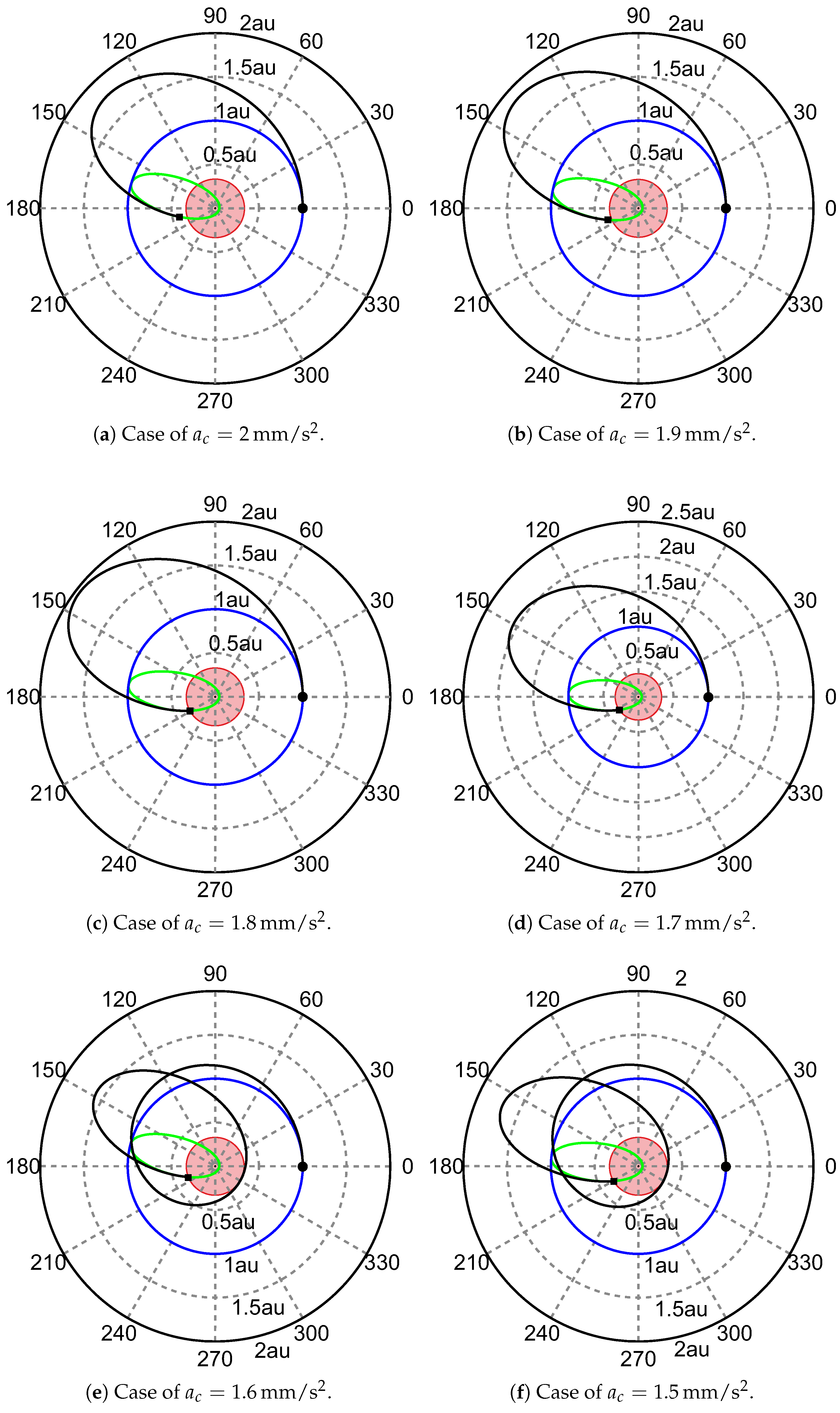
This behavior is clearly illustrated in Figure 5, which shows the optimal transfer trajectory as a function of the characteristic acceleration within the selected set of values. In particular, the graphs reassumed in Figure 5 highlight the differences between the case when $a_c=1.7\mathrm{mm}/{\mathrm{s}}^2$ and that when $a_c=1.6\mathrm{mm}/{\mathrm{s}}^2$ in terms of trajectory topology; see Figure 5d,e, respectively. Note that, for the assigned characteristics of the target orbit, $a_c=1.6\mathrm{mm}/{\mathrm{s}}^2$ represents a sort of threshold value of $a_c$ below which the optimal transfer trajectory requires at least a full revolution around the Sun and the path constraint of Equation (3) gives a tangent condition at one (or more) points.

For exemplary purposes, consider a spacecraft with a characteristic acceleration below such a threshold value, i.e., $a_c=1.5\mathrm{mm}/{\mathrm{s}}^2$. In this case, the time variation of the spacecraft states are those reported in Figure 6a, where the red dash line in the upper graph of the figure (corresponding to the radial distance r) represents the constraint on the minimum solar radius of Equation (3). According to Figure 5f, the Sun–spacecraft distance is just equal to $r_m$ at two different points, one coinciding with the final spacecraft position (i.e., the point occupied at $t=t_f$), and the other corresponding to the spacecraft position at about $t=t_f/2$, when the transfer trajectory becomes tangent to the forbidden region, as sketched in Figure 5f. From Figure 6a, it is clear that the maximum transverse component of the spacecraft velocity v is reached just at that tangent point. This is by no means a surprising result, because the inner part of the trajectory (when $r<r_{\oplus }$) is used by the spacecraft to increase the osculating orbit aphelion radius $r_a$, so that the succeeding part of the transfer trajectory has a behavior similar to that obtained for high values of $a_c$; see Figure 5a,b.

Figure 6b shows the time variation of the characteristics of the spacecraft osculating orbit, in term of semimajor axis a, eccentricity e, perihelion radius $r_p$, and aphelion radius $r_a$. 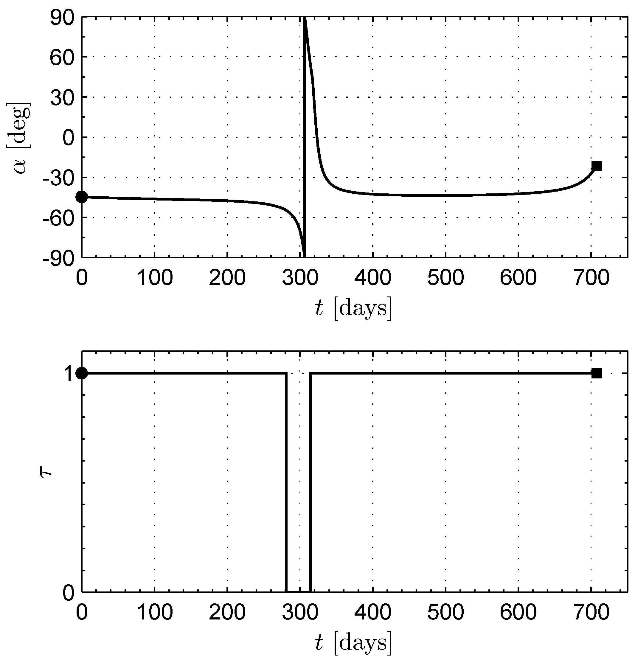In particular, the first two graphs of Figure 6b confirm that the elliptic target orbit is reached at the end of the transfer, while the other two plots indicate that the optimal transfer trajectory has a coasting phase (that is, a phase in which $\tau =0$) in the neighborhood of the tangent point with the circular forbidden zone. The presence of such a coasting phase is confirmed by Figure 7, which shows the time variation of the two control variables $\alpha$ and $\tau$. Please note that the duration of the coasting phase is small (about $33\mathrm{days}$) when compared with the total flight time of $707\mathrm{days}$.

4. Conclusions

The use of an advanced propellantless propulsion concept such as the E-sail allows complex interplanetary transfer trajectories and high-energy mission scenarios to become a viable option and a promising alternative to more conventional choices, usually based on chemical systems. In this context, this paper has analyzed the problem of reaching a highly elliptic heliocentric orbit with a perihelion distance of a few solar radii, to complete a campaign of in situ observation of the Sun’s upper atmosphere. This particular orbit, whose characteristics are consistent with the guidelines of the current PSP mission, can be reached with a flight time smaller than 2 years using a medium-performance E-sail. The preliminary design of the (two-dimensional) interplanetary transfer trajectory has been obtained as the solution to a minimum-time control problem that constraints the spacecraft to not enter inside a specified spherical region around the Sun to avoid excessive thermal loads on the E-sail charged tethers. This kind of (interior) path constraint makes the trajectory design a non-trivial problem to solve. In fact, the presence of a forbidden region that includes a non-negligible part of the target orbit reduces the admissible variation of the rendezvous point on the final orbit to a narrow range of (final) true anomalies. Nevertheless, feasible solutions are possible and the simulation results show that an E-sail with a characteristic acceleration of about $1.5\mathrm{mm}/{\mathrm{s}}^2$ may send the probe on the required target orbit without the need for several Venus flybys, as in the case of the PSP mission.