1. Introduction
In recent years, with the increasing need for special photography in film and television, agriculture, firefighting, rescue and other fields, multi-rotor unmanned aerial vehicles (UAV) have been widely used in practice due to their reliability and stability, small size, and ease of handling [
1,
2,
3]. With the widespread application of multi-rotor UAVs, multi-rotor-UAV navigation technology has also gradually attracted the attention of various research institutions. Due to the small size and light weight of multi-rotor UAVs, it is difficult to use larger navigation devices to multi-rotor UAVs; therefore, the current multi-rotor UAV navigation mostly uses a combination of GPS and inertial navigation system (INS) navigation [
4,
5,
6]. However, GPS navigation is essentially a type of radio navigation that inevitably communicates with the outside world. Due to the instability of the GPS signal, multi-rotor-UAV crashes occur from time to time. Meanwhile, visual-navigation technology based on optical flow directly processes continuous image sequences by transforming the optical-flow-field information calculated by the optical flow method directly into motion-field information through a mathematical model. The navigation system using the optical-flow method is easy to implement and the real-time performance is guaranteed, which has become an important research direction for visual navigation. With the development of microelectronics, CMOS cameras are moving toward miniaturization, and the development of optical-flow-navigation technology has therefore reached a new stage. In 2017, McGuire, K. et al. [
7] implemented optical-flow autonomous navigation on a 40-gram UAV. In 2020, Back, S. et al. [
8] used a neural-network-based optical-flow algorithm to track bicycle-path-obstacle avoidance, which enables the UAV to handle various situations encountered while traveling on a fixed track by combining route tracking, interference recovery, and obstacle avoidance. The feasibility of the method was also verified using dataset simulations and actual flight experiments.
To solve the problems of low accuracy and poor stability of most existing optical-flow-method navigation algorithms, a semi-physical simulation platform for UAV visual navigation needs to be designed and developed before outdoor flight tests of the visual-navigation algorithms can be conducted. The semi-physical-simulation-test validation will be conducted through this platform to improve the algorithm’s iteration speed while avoiding flight accidents and economic losses in the real outdoor tests caused by algorithm errors. When the stability, real-time and accuracy of the optical-flow-method navigation algorithm meet the test-flight requirements, the actual flight test will be conducted.
The existing simulation tests are mainly divided into three categories: numerical computer simulation, hardware-in-the-loop (HIL) simulation and semi-physical simulation [
9,
10,
11]. Numerical computer simulation can realize the digital simulation of UAV flight by creating 3D models, as well as simulation scenarios. Computer numerical simulation is also used in the fields of flight aircraft planning, as well as flight-simulation demonstration [
12,
13,
14]. Although computer numerical simulation can significantly reduce the cost, it usually ignores the effects of the interactions between the various physical components of the actual UAV system; therefore, the simulation results usually differ from the actual situation.
The hardware-in-the-loop simulation system, which includes the simulation computer and a simplified version of the simulation hardware, is the second stage of flight simulation [
15,
16,
17,
18]. For example, KASSANDRA, a distributed architecture developed by Euroworks, allows communication between different simulation tools, and real hardware units can be seamlessly integrated with simulation units to achieve more accurate simulation [
19]. A hardware-in-the-loop simulation of the UAV proportional–integral–derivative (PID) controller is proposed [
20]. The controller used was a PID controller, tuned using the Ziegler–Nichols method. The implementation of the hardware-in-the-loop-simulation (HILS) can be performed after the design of control systems for UAVs is completed. These simulation systems have deterministic real-time simulation capability as well as data-acquisition capability, and when combined with computer-simulation technology, can more realistically simulate the verification of aircraft flight conditions in various environments. Hardware-in-the-loop simulation systems use computer models instead of some sensors or actuators, which have large errors compared to real sensors. Such systems cannot provide real-world visual feedback and are not suitable for the visual-navigation testing of UAVs.
A semi-physical simulation system is a system that combines the real test objects and sensors with some physical models from the simulation computer. The resulting simulation system also provides a realistic simulation of the natural environment [
21,
22,
23]. Compared with the hardware-in-the-loop simulation system, it has a higher degree of simulation and is the closest indoor-simulation system to real tests. The semi-physical simulation can directly represent the parts of the flight system that cannot be accurately described by mathematical models with physical objects. The simulation of UAV flight-motion characteristics is also the focus of semi-physical simulation, and the three-axis rotary table and five-axis rotary table are commonly used to simulate the flight attitude. The S-458R-5Se infrared and laser-simulation rotary table developed in the United States can achieve 2″ accuracy in its simulated turning angle [
24]. In 2018, Yonsei University in South Korea used motion-capture cameras and two pneumatic spacecraft simulators to simulate spacecraft-thrust control on a smooth aluminum surface to validate tests of autonomous navigation algorithms [
25], but this system lacks
Z-axis motion simulation and
X- and
Y-axes rotation. Most of the existing large rotary tables can only be used to realize the simulation of flight attitude due to the limited number of degrees of freedom, and cannot simulate the trajectory and flight scene, which is not suitable for testing the UAV visual-navigation algorithm.
Motion-capture systems are also very common means of testing navigation algorithms on unmanned systems. For example, the OptiTrack Prime ×13 motion-capture camera has a resolution of 1.3 MP, 3D accuracy of +/−0.2 mm, and native frame rate of 240 FPS. The data-transmission latency for the motion capture-systems is typically in the millisecond range, such as 2–3 ms for systems based on the OptiTrack Prime ×13 motion capture camera. If using the EtherCAT-based semi-physical simulation platform, data-transmission latency can be reduced to microsecond range and the repeat-positioning accuracy can be further improved.
The innovations of this paper are as follows:
Proposing a novel UAV semi-physical-simulation platform architecture that can simulate the flight attitude of a UAV in a three-dimensional space of 4 × 2 × 1.4 m realistically.
The real-time flight-attitude simulation is realized in a real physical environment and virtual-animation space, and the flight tests of various scenes are realized by combining with the simulation-environment sandbox.
The repeated-positioning accuracy and dynamic-positioning accuracy meet the simulation requirements of high-precision visual UAV navigation.
The rest of this paper is organized as follows: in the second section, optical-flow-field theory and its application to navigation are introduced. In the third section, a mathematical model of the simulation platform and the mechanical structure’s design is presented. In the fourth section, the structure of the semi-physical simulation platform is studied and analyzed to provide the framework for the control system, and the adapted upper-computer software is also presented. In the fifth section, the performance tests of the semi-physical simulation platform, dynamic performance and optical flow are reported. In the last section, the results and limitations of this study are presented, and an outlook on future research directions is given.
2. Optical-Flow-Field Theory and Its Application to Navigation
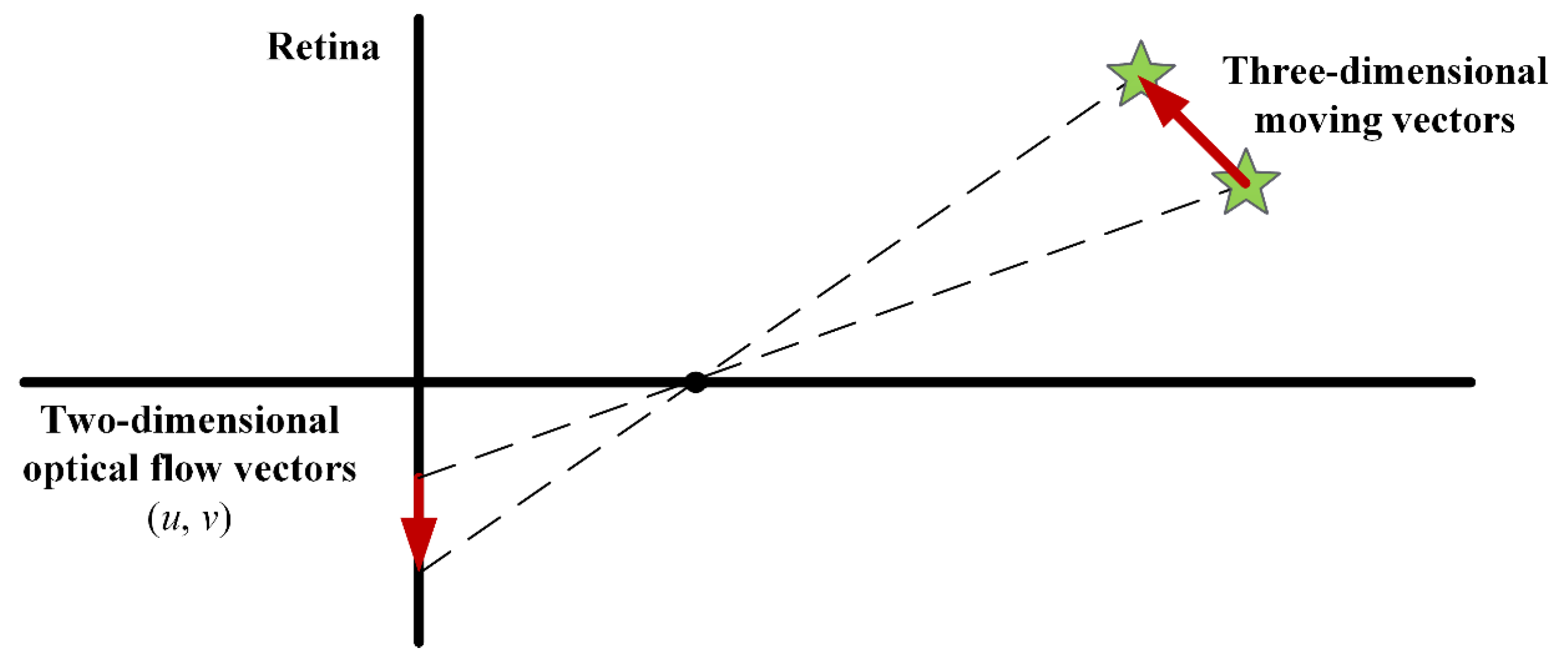
The basic concept of the optical-flow method is shown in
Figure 1. It was first proposed by Gibson, J.J. [
26] in 1950 and is an important branch of computer vision. When the human eye looks at a moving object, the object forms constantly changing images on the retina, and these images move across the retina, creating optical flow. The ultimate goal of the optical-flow method is to calculate the object’s motion information contained in two adjacent images through certain mathematical methods.
The existing method for estimating the optical flow-field assumes that the following assumptions are met: 1. Grayscale is stable and unchanged. 2. Time continuity or the movement is “small movement”. The operation of the navigation system depends on the accuracy and high update rate of the navigation data, so the optical-flow algorithm for navigation should guarantee not only the accuracy, but also the computational efficiency. The Lucas–Kanade (LK) optical-flow algorithm [
27] and the edge histogram-based matching algorithm are suitable for optical-flow navigation due to the fast computation speed and sparse optical-flow output. In addition to the assumption of small movements and the principle of luminance conservation, the principle of small-window-optical-flow consistency is also assumed. The assumption of optical-flow consistency is used as a basis to create a matrix of the neighborhood pixel system, through which the motion of the central pixel point in both directions is calculated. When the neighborhood pixel size is n × n, the following set of equations is obtained.
where
,
, and
is the partial derivative of the grayscale of the pixel points in the image with respect to the
x,
y, and
t directions. The equation can be abbreviated as follows:
The least-squares method is used to solve this superdeterministic problem:
When
is invertible, the value of the optical flow is obtained by solving this equation:
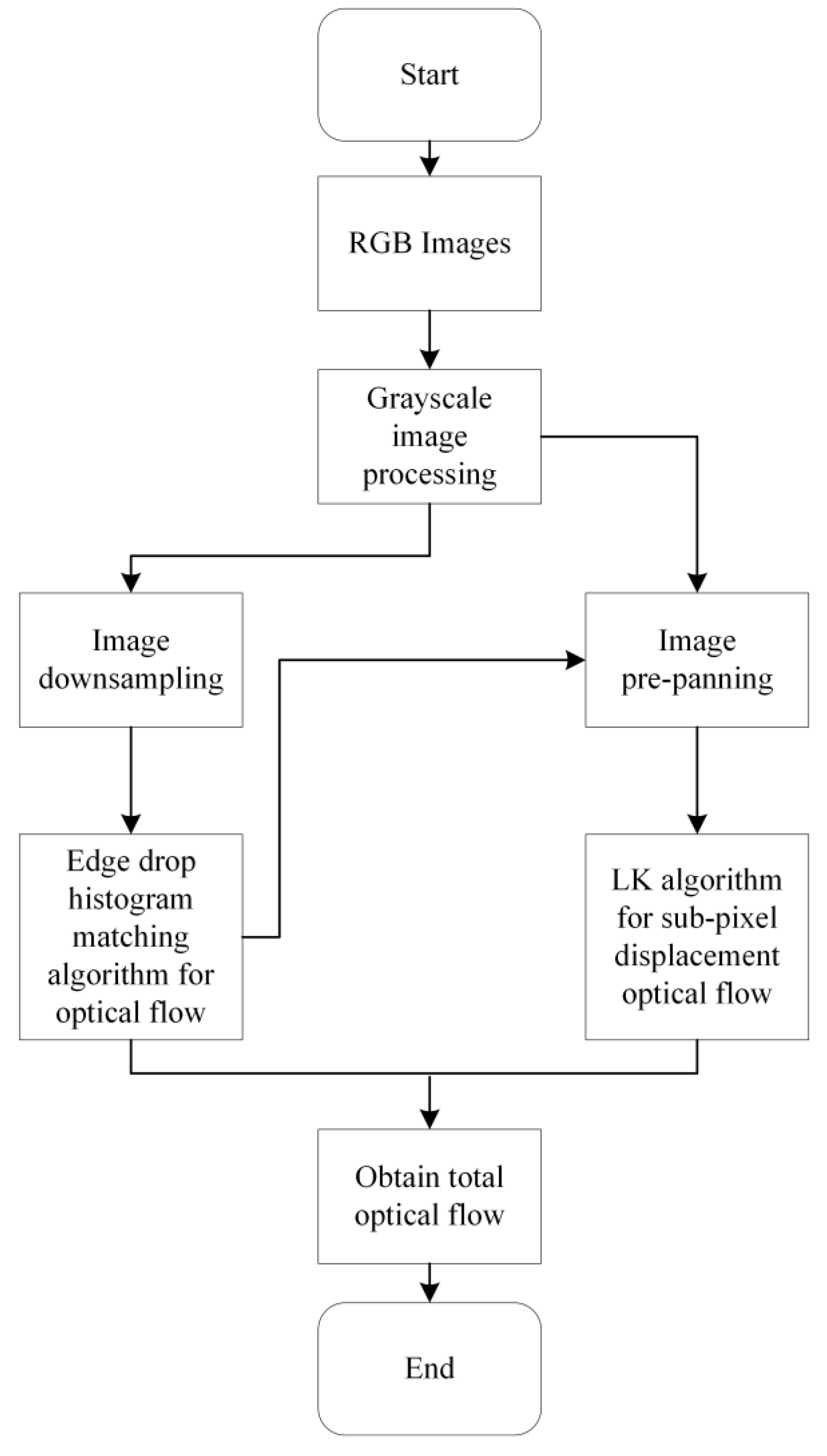
The optical-flow algorithm based on edge-histogram matching greatly reduces the complexity of the algorithm and improves the speed of optical-flow calculation.
Figure 2 shows the flow chart of the algorithm. By assuming the consistency of the optical flow, the LK optical-flow method combines the information of the neighboring pixels, eliminating the uncertainty of the optical-flow equation. However, the LK optical-flow method also has inherent shortcomings, such as the problem of large displacement and the problem of optical-flow inconsistency, which need to be improved by taking appropriate measures in the actual application. The basic steps of the large-displacement optical-flow algorithm based on edge-histogram matching are as follows.
Capture the image, record the continuous video frames with the camera, and save the two adjacent frames as and .
Grayscale the two adjacent frames to obtain and .
The grayscale image is downsampled to obtain and .
Use the image edge-histogram-matching algorithm to obtain the coarse optical flow .
The i times of the obtained coarse optical flow are used as translations to perform pre-panning of and to obtain and .
Solve the optical flow between and to obtain , using the LK optical-flow algorithm.
The total optical flow is obtained by summing and .
For monocular cameras, to obtain a more accurate displacement map, the distance between the camera and the captured feature point must be known. When validating flight-navigation algorithms, having more accurate distances available in real time is important for algorithm optimization.
3. Mathematical Model of the Simulation Platform and the Mechanical Structure Design
Hardware-in-the-loop simulation and semi-physical simulation tests can usually be conducted before carrying out the real indoor or outdoor flight tests of UAVs. Using a semi-physical simulation platform for flight testing can reduce the collisions caused by uncontrollable factors during flights, avoid damaging UAVs, and improve testing efficiency. Meanwhile, the EtherCAT-based semi-physical simulation platform has lower data-transmission latency. The data-refresh cycle is less than 100 us using EtherCAT bus. The synchronization accuracy of each slave-node device can be guaranteed to be less than 1 us. It is much higher than the motion-capture system, which has a data-transmission latency in the millisecond range. In addition, the repeat positioning error of the semi-physical simulation system is usually lower than that of the motion-capture system.
This simulation platform can simulate many types of UAV, and the following is an example of a quadrotor UAV. Based on the dynamic model of the UAV and the characteristics of the optical-flow-method navigation algorithm, the UAV’s semi-physical simulation platform is designed and built, and at the same time, an analysis of the dynamic performance is performed.
3.1. Quadrotor UAV-Dynamics Modeling
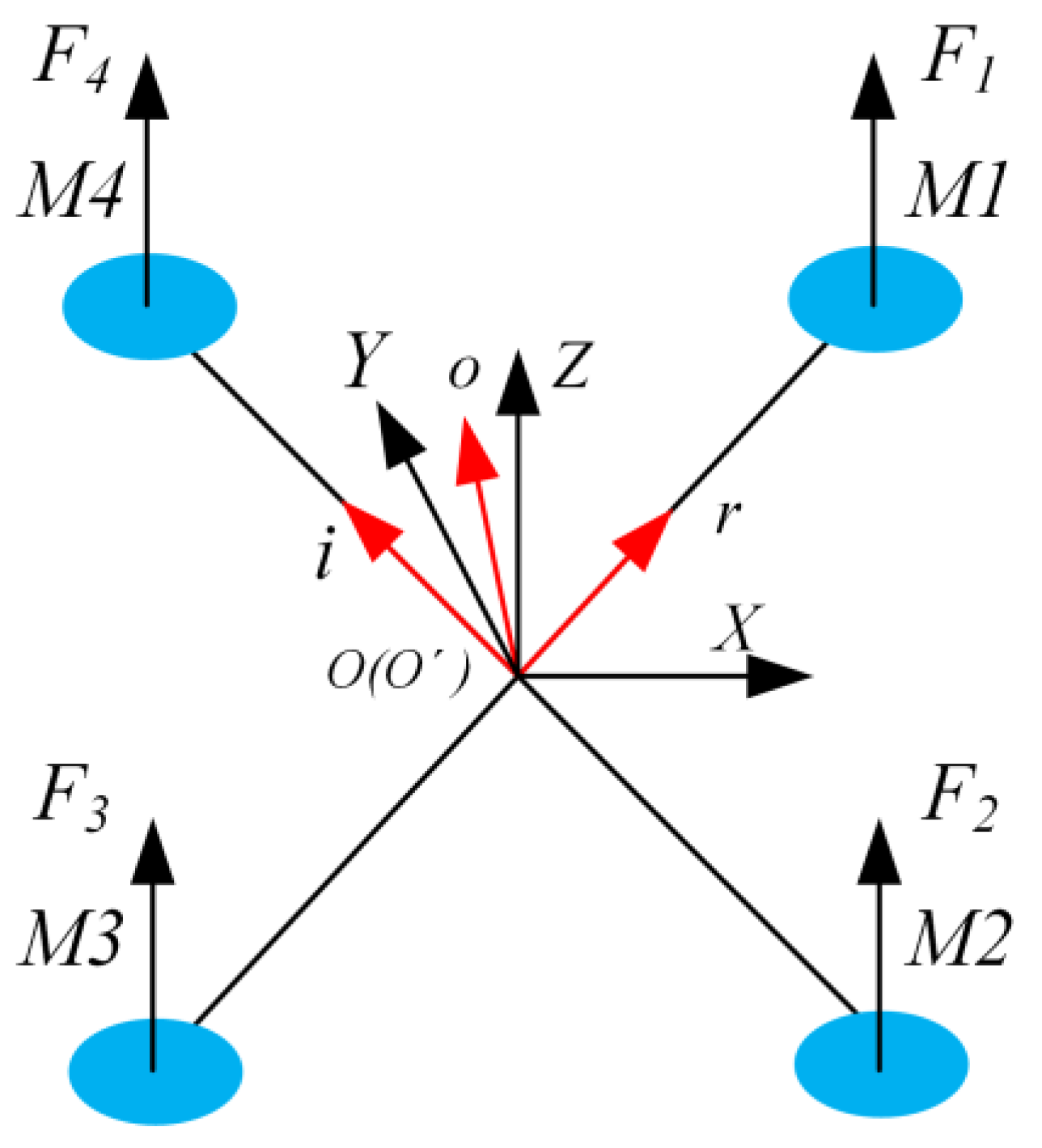
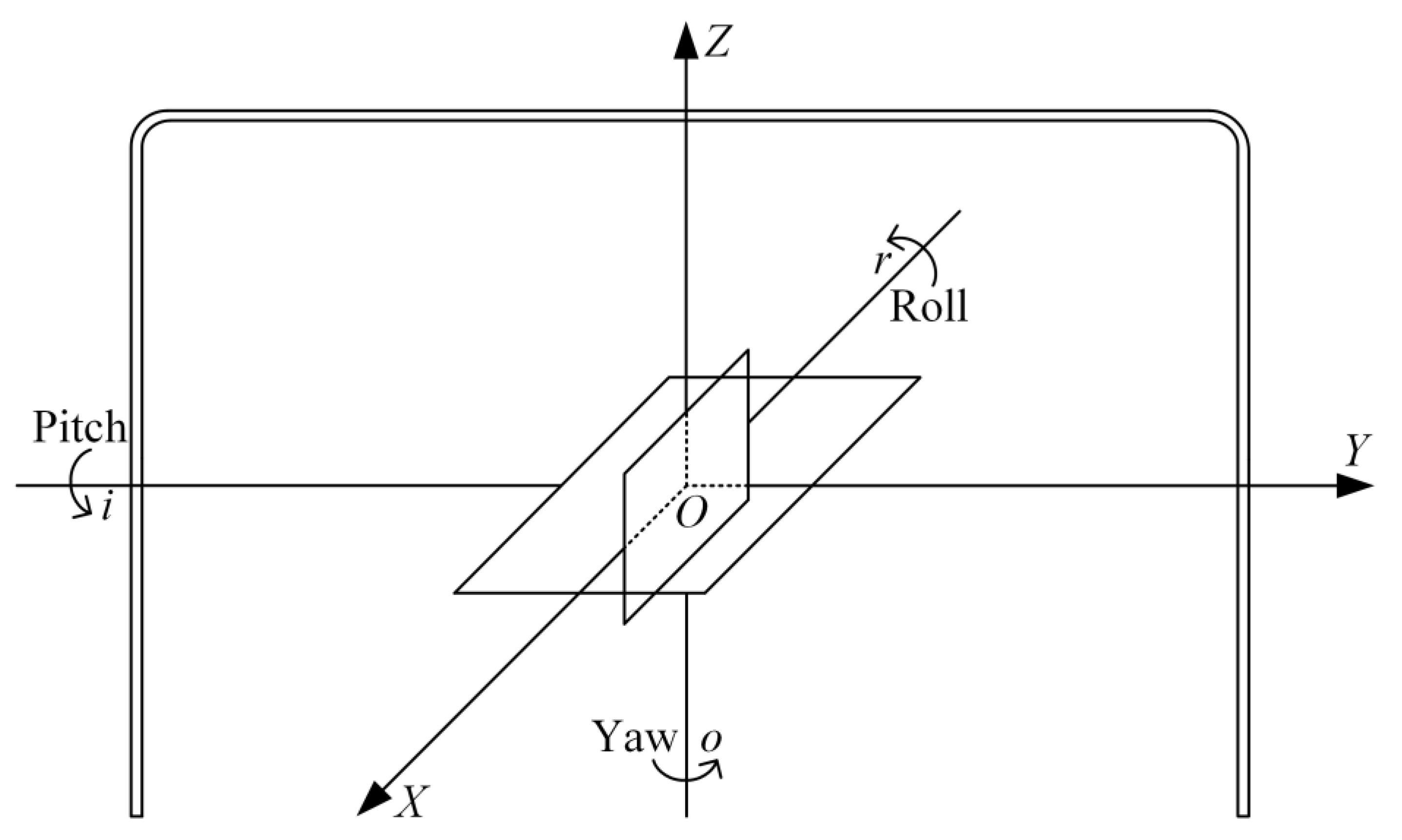
Based on the flight dynamics of the quadrotor UAV, the attitude equation of the quadrotor can be derived as follows. The inertial coordinate system (OXYZ) and quadrotor coordinate system (O’rio) are shown in
Figure 3. Define the following quantities: angle of rotation
of the roll axis; angle of rotation
of the pitch axis; angle of rotation
of the pitch axis. The angular velocities of the
,
, and
are
,
, and
, respectively. The angular acceleration of the
,
, and
are
,
, and
, respectively. The
M1,
M2,
M3, and
M4 denote the drive motors on each axis of the quadrotor. The
,
,
, and
are the lift forces generated by the four motors. The
,
, and
denote the rotational inertia of each axis of the quadrotor UAV in its coordinate system,
is the rotational speed of each axis motor,
is the rotational air drag, and
is the distance from the center of motor rotation to the origin of the quadrotor coordinate system. To simplify the calculation, the inertial coordinate origin is coincident with the origin of the UAV coordinate system. The attitude equation of the quadrotor can be derived from the flight dynamics of the quadrotor UAV as follows [
28]:
The mathematical model of the drone position is as follows:
where
,
, and
represent the displacement on the corresponding axis in the quadrotor coordinate system, respectively,
represents the lift coefficient,
is the mass of the UAV,
is the acceleration due to gravity,
,
, and
are the air-drag coefficients of the UAV along the
,
, and
axes,
,
, and
represent the system perturbations of the UAV along the
,
, and
axes. From the analysis of Equations (5) and (6), it can be observed that the attitude of the quadrotor UAV must change whenever its motion state in the three-dimensional space changes. Therefore, to simulate the flight of the UAV, a mechanical structure with six degrees of freedom in a certain space must be designed.
3.2. Mechanical-Structure Design
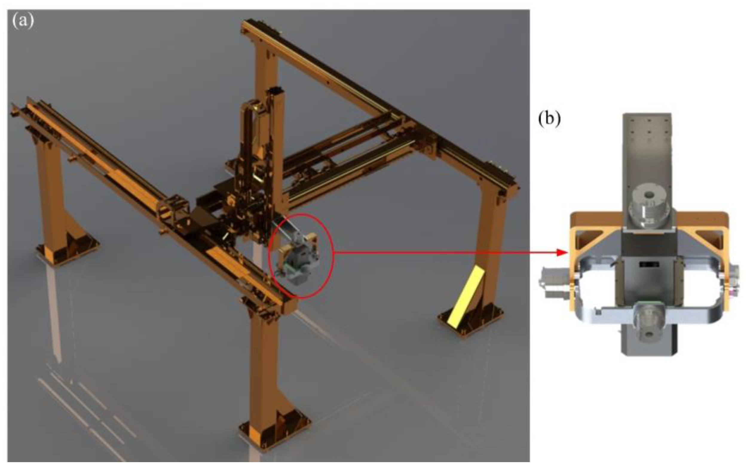
To better perform UAV testing, a three-axis rotary table was combined with a three-axis translation table in this study. The structure is capable of linear displacement in three directions and can have six degrees of freedom in a given space. Its three-dimensional structure is shown in
Figure 4.
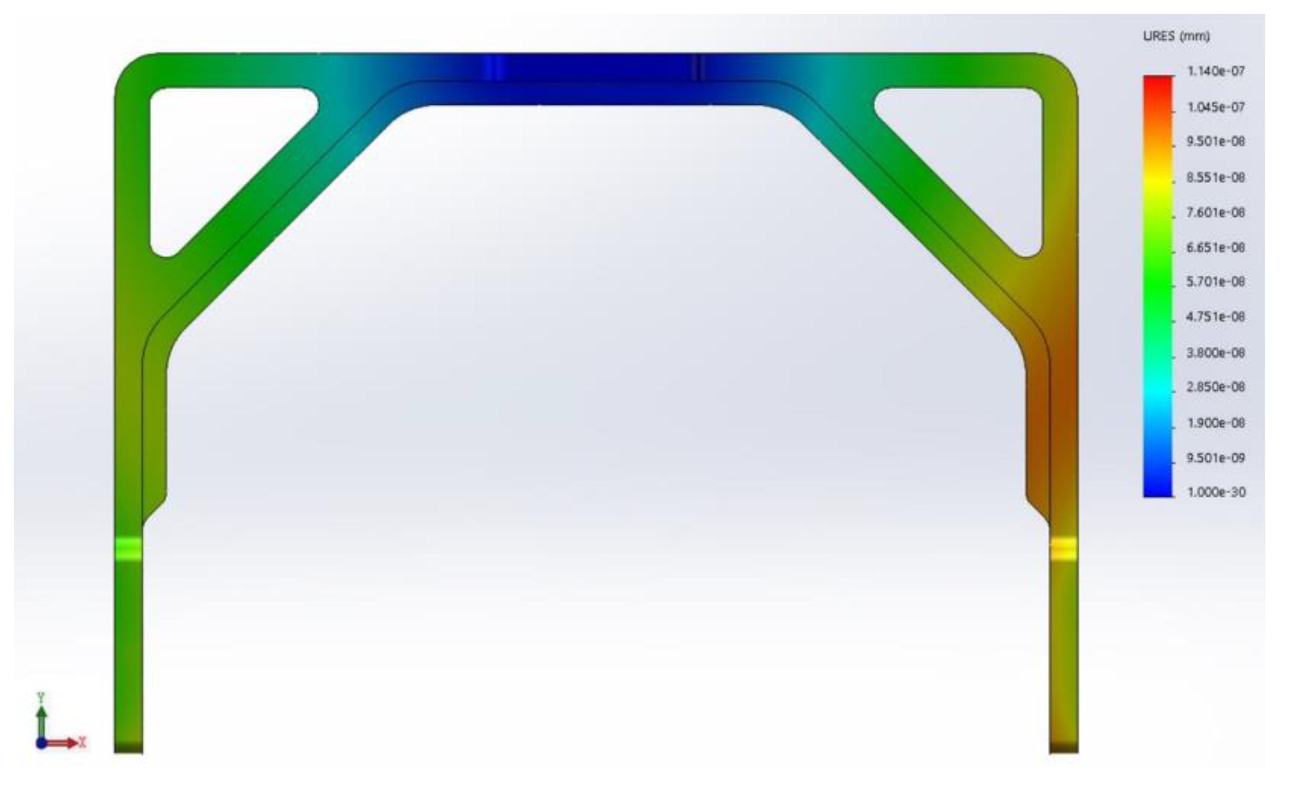
In the simulation of quadrotor UAV flight, the end of the rotary table must support the cameras, while the rotary table is affected by the rotational inertia during operation, which imposes certain requirements on the structural strength of the rotary table.
In this study, the conventional rotary-table structure is improved to achieve a lightweight design without changing its load-bearing capacity, as shown in
Figure 4b. The mechanical-performance analysis of the yaw-axis frame is shown in
Figure 5. When the rotary table is suspended on the translation table, the outer frame is subjected to the maximum load. The finite-element analysis shows that the end deformation at maximum load is only 1.14 × 10
−7 mm, which meets the requirements of high-precision simulation.
3.3. Coupled-Dynamics Model of a Six-Axis Simulation Platform
The mechanical structure of the simulation platform designed in this paper mainly consists of two subsystems: a three-axis translation table and a three-axis rotary table. The three rotating frames of the rotary table are coupled together, and their motions influence each other. The coupling mainly includes inertial coupling and dynamic coupling. Inertial coupling refers to the rotational inertia that varies within a certain range during the motion of the rotary table; kinetic coupling refers to the cross-coupling of the moments of inertia and gyroscopic effects between the frames. Therefore, the coupling between the axes must be calculated.
Figure 6 shows the coordinate relationship between the three-axis translation table and the three-axis rotary table.
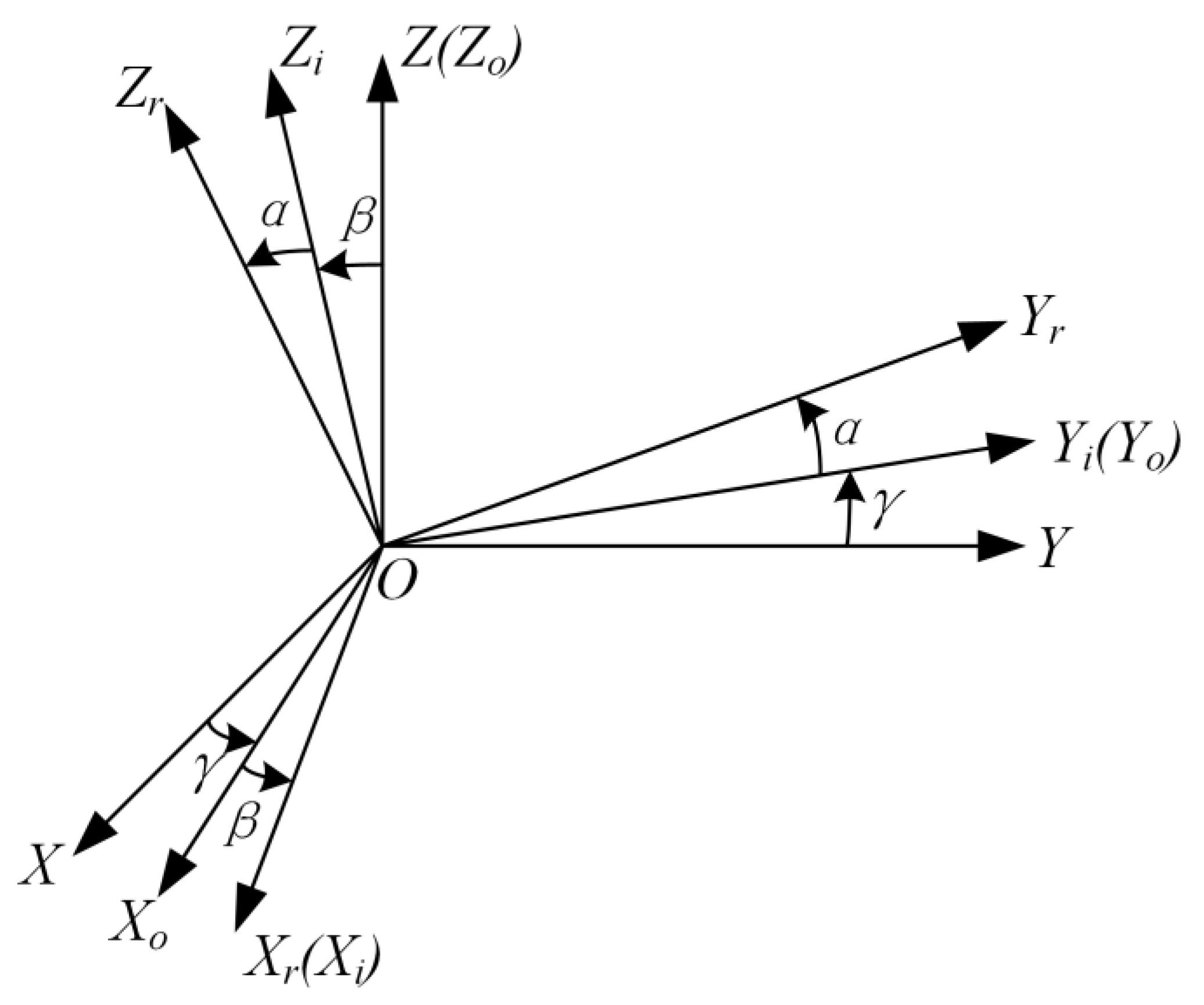
The coordinate relationship between the three axes of the three-axis rotary table when they are not orthogonal is shown in
Figure 7. The coordinate system
represents the geodetic coordinate system, the coordinate system
represents the yaw-axis-frame coordinate system, the coordinate system
represents the pitch-axis-frame coordinate system, and the coordinate system
represents the roll-axis-frame coordinate system. When the three axes are orthogonal to each other, the yaw axis (including the pitch and roll axis frames) is rotated counterclockwise by one angle
about its axis of rotation
. The pitch axis (including the roll-axis frame) is rotated counterclockwise by an angle
around its axis of rotation
. The roll axis rotates counterclockwise by an angle
around its rotation axis
. This results in the coordinate-relationship diagram in
Figure 7. The angular velocities of the roll, pitch, and yaw axes are
,
, and
, respectively. The angular of the roll-, pitch-, and yaw-axes accelerations are
,
, and
, respectively. The
represents the rotational inertia of the corresponding axis, where
N =
X,
Y, and
Z. The
represents the rotational inertia of the corresponding axis, where
M =
X,
Y, and
Z,
n =
i and
r.
The rotational inertia
of the roll-axis frame with respect to the axis
can be calculated as follows:
The rotational inertia
of the roll-axis frame with respect to the axis
can be calculated as follows:
The rotational inertia
of the roll-axis frame with respect to the axis
can be calculated as follows:
The rotational inertia
of the pitch-axis frame with respect to the axis
can be calculated as follows:
The rotational inertia
of the pitch-axis frame, including the roll-axis frame, with respect to the pitch axis
can be calculated as follows:
From Equation (11), the inertia
of the yaw frame, including the roll frame and the pitch frame, with respect to the yaw axis
can be deduced as follows:
The value of
can be obtained by substituting the approximate value of moment of inertia of the three axes in
Table 1 with respect to each axis of rotation into Equation (12). To facilitate the calculation, the motion of each rigid body is solved separately, after which the mutual influence is calculated. The angular-velocity vectors of the three rigid bodies are defined as follows.
is the angular-velocity vector of the roll axis with respect to the pitch axis.
is the angular-velocity vector of the pitch axis with respect to the yaw axis.
is the angular-velocity vector of the yaw axis with respect to the geodetic coordinate system. According to the Gothic rotation theorem [
29], we obtain:
where
is the moment of momentum of the rigid body,
,
, and
represent the moment of momentum on the
x,
y, and
z axes of the rigid body, and
,
, and
are the unit vectors on the
X,
Y, and
Z axes.
Let
be the moment to which the rigid body is subjected. According to the momentum-moment theorem [
29] we can obtain:
The Eulerian=dynamics equation for a rigid body is obtained by the union of Equations (13) and (14).
The final result is as follows:
3.4. AC-Servo-Motor Mathematical Model
The AC servo system has a high torque ratio and can achieve both rapid start-up and deceleration. The motor chosen in this paper is a permanent-magnet AC servo motor, and the torque equation of the motor
is calculated according to [
28]:
where
is the motor power,
is the coupled magnetic chain of the rotor magnets on the stator,
and
are the direct- and alternating-axis main inductance of the permanent magnet synchronous motor, and
and
are the alternating and direct axis components of the stator-current vector.
To simplify the control system, take
and
. The torque equation of the permanent-magnet AC motor is transformed into:
Since
is the motor constant, the torque equation is simplified as:
where
is the torque constant of the AC servo motor. An examination of the motor-product manual shows that the torque constants of the roll and pitch axes are 4 kg·fm/A, and the torque constant of the yaw axis is 4.2 kg·fm/A. The AC motor can be simplified to a DC-motor model to realize the decoupling of the control parameters of the three-phase permanent magnet synchronous motor and achieve the purpose of vector control. By coupling Equations (16)–(18) and (21) and neglecting the minimal quantities, we obtain:
where
,
, and
are the currents along the
r,
i, and
o axes. Assuming that:
The dynamic system of the rotary table can then be converted into the following form:
It can be seen that the three-axis rotary table is a non-linear system with three inputs and three outputs, and the individual rotating axes are coupled together. Therefore, to improve the control accuracy, the system must be decoupled for calculation.
The system can be decoupled using state feedback and dynamic-feedback compensation. For Equation (26), let:
where
,
, and
are the current corrections for the
r,
i, and
o axes. Next, there are:
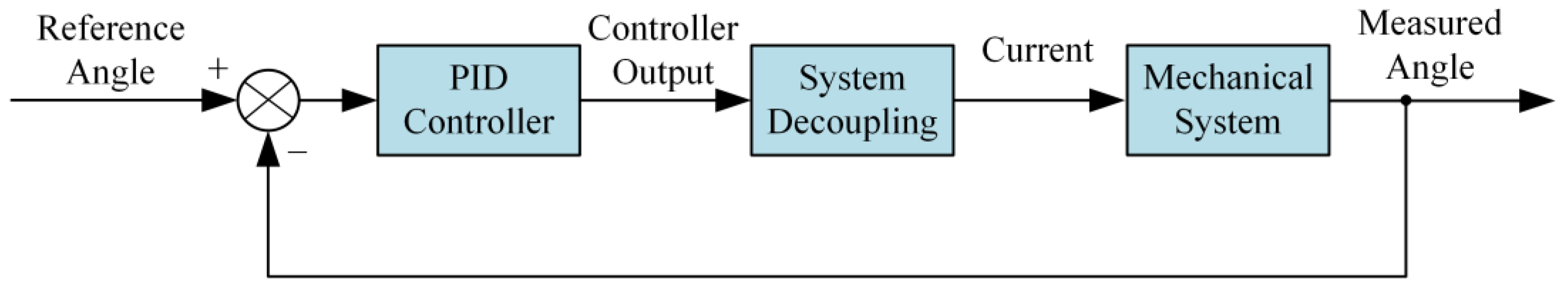
If Equations (30)–(32) are connected in series as a dynamic-compensation and state-feedback decoupling network before Equation (26), the system can be reduced as follows:
In this case, the system is a single-input, single-output system with inputs
,
, and
and outputs
,
, and
. The decoupling network is connected in series with the control network, as shown in
Figure 8.
5. Experimental Results and Discussion
In this chapter, the repeat-positioning accuracy, cumulative-positioning accuracy, and dynamic performance of the simulation platform are tested and verified.
5.1. Steady-State Performance Test
To test the steady-state performance of the simulation platform, a laser interferometer was used in this study to test the linear-axis running range (XYZ), repeat positioning accuracy, cumulative positioning accuracy, linear-axis running speed, and linear-axis running acceleration of the three-axis translation table. In addition, the rotary-axis running range (UVW), repetitive positioning accuracy, rotary-axis running speed, and rotary-axis running acceleration of the three-axis rotary table were also tested.
The test method for the accuracy of the three-axis translation table involved cyclic and continuous measurement in the positive and negative directions of the X-, Y, and Z-axes. Three convergences were made in each direction for each target position Pi. The actual arrival position was measured with a laser interferometer and the position deviation was calculated. For the cumulative error, the initial target position was determined by the motion on one axis and moving the moving part 1000 m. The moving part returned to the initial target position. The actual arrival position was measured with the laser interferometer and the position deviation was calculated as the cumulative positioning accuracy.
The test method for the accuracy of the three-axis rotary table involved the use of a laser interferometer and a supporting indexing table to calibrate the rotary axis. The indexing table was installed at the center of the rotary axis. The indexing table and the rotation center of the rotary axis were adjusted by applying the table method, so that the radial circular run-out value did not exceed 0.02 mm. The angle reflector was installed on the indexing table, and the angle reflector was made surface perpendicular to the laser beam. The angular interferometer was installed in the optical path so that it was parallel to the angular reflector boarding, the laser head was panned so that the laser beam was collimated. The rotation speed of the control system was set and the target position, the overtravel amount, the stopping time at the target point, and the number of cycles were determine. Continuous measurements were cycled in the positive and negative directions of the U, V, and W axes. Three convergences were performed in each direction for each target position Pi. The actual arrival position was measured with the laser interferometer and the position deviation was calculated. In the tests of the cumulative positioning accuracy, the corresponding axis was moved continuously for a distance of 1000 m or more to determine this value.
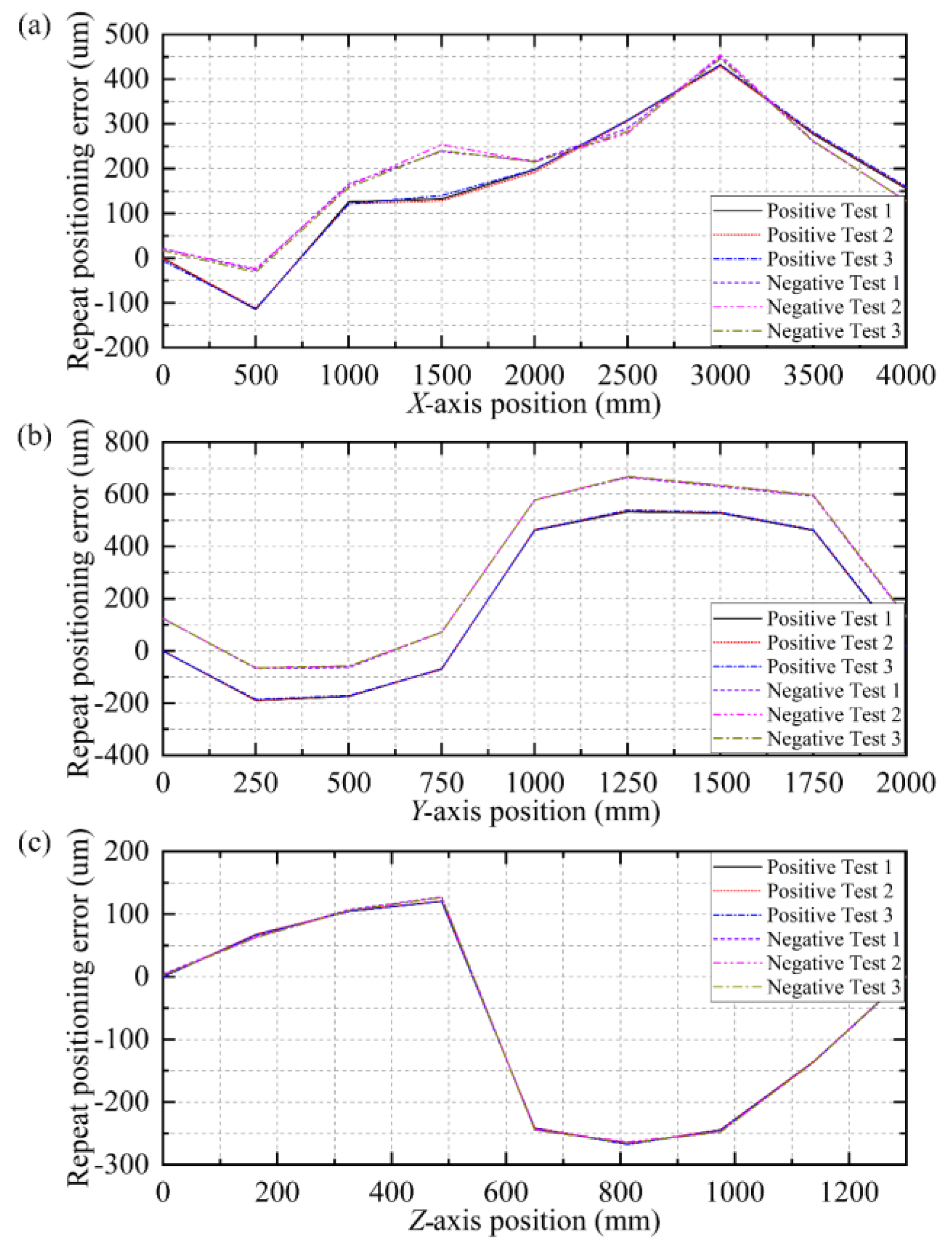
The
X-axis was repeatedly measured three times according to the specified test method, and the test results are shown in
Figure 15a. The repeat-positioning accuracy was 0.033 mm, and the reverse difference was 0.11 mm. The cumulative-positioning accuracy was 0.02 mm/1000 m after moving the
X-axis for 1000 m. As the corresponding axes needed to be made to actually move for 1000 m or more, this test was time consuming, usually between half a day and a day. The
Y-axis was measured repeatedly three times according to the specified test method, and the test results are shown in
Figure 15b. The repeat positioning accuracy is 0.012 mm, and the reverse difference is 0.11 mm. The
Z-axis was measured repeatedly three times according to the specified test method, and the test results are shown in
Figure 15c. The repeat-positioning accuracy is 0.004 mm, and the reverse difference is 0.007 mm.
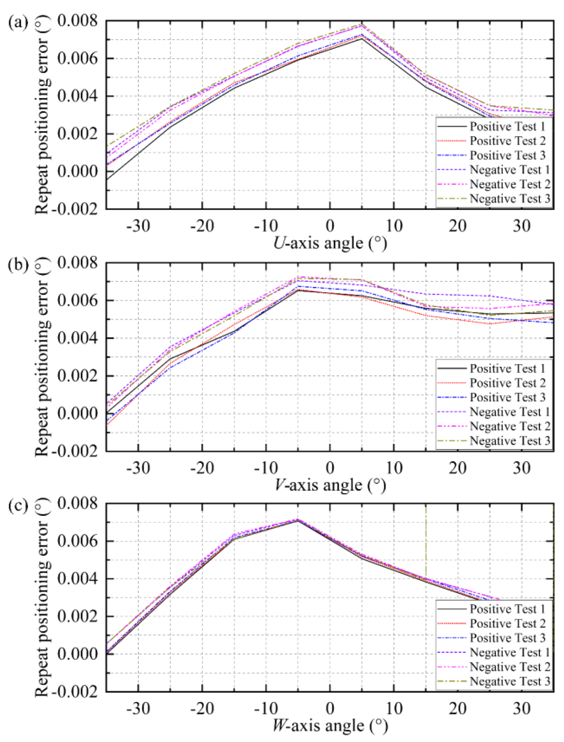
According to the specified test method of repeating the measurement of the
U-axis three times, the test results are shown in
Figure 16a; the repeat-positioning accuracy was 0.002° and the reverse difference was 0.001°. According to the established test method of repeating the measurement of the
V-axis three times, the test results are shown in
Figure 16b; the repeat positioning accuracy was 0.002° and the reverse difference was 0.001°. According to the specified test method of repeating the measurement of the
W-axis three times, the test results are shown in
Figure 16c; the repeat-positioning accuracy was 0.006° and the reverse difference was 0.001°. The measurement results are shown in the following table.
Table 4 shows the steady-state-performance test results of the three-axis translation table and the three-axis rotary table.
5.2. Dynamic Performance Test
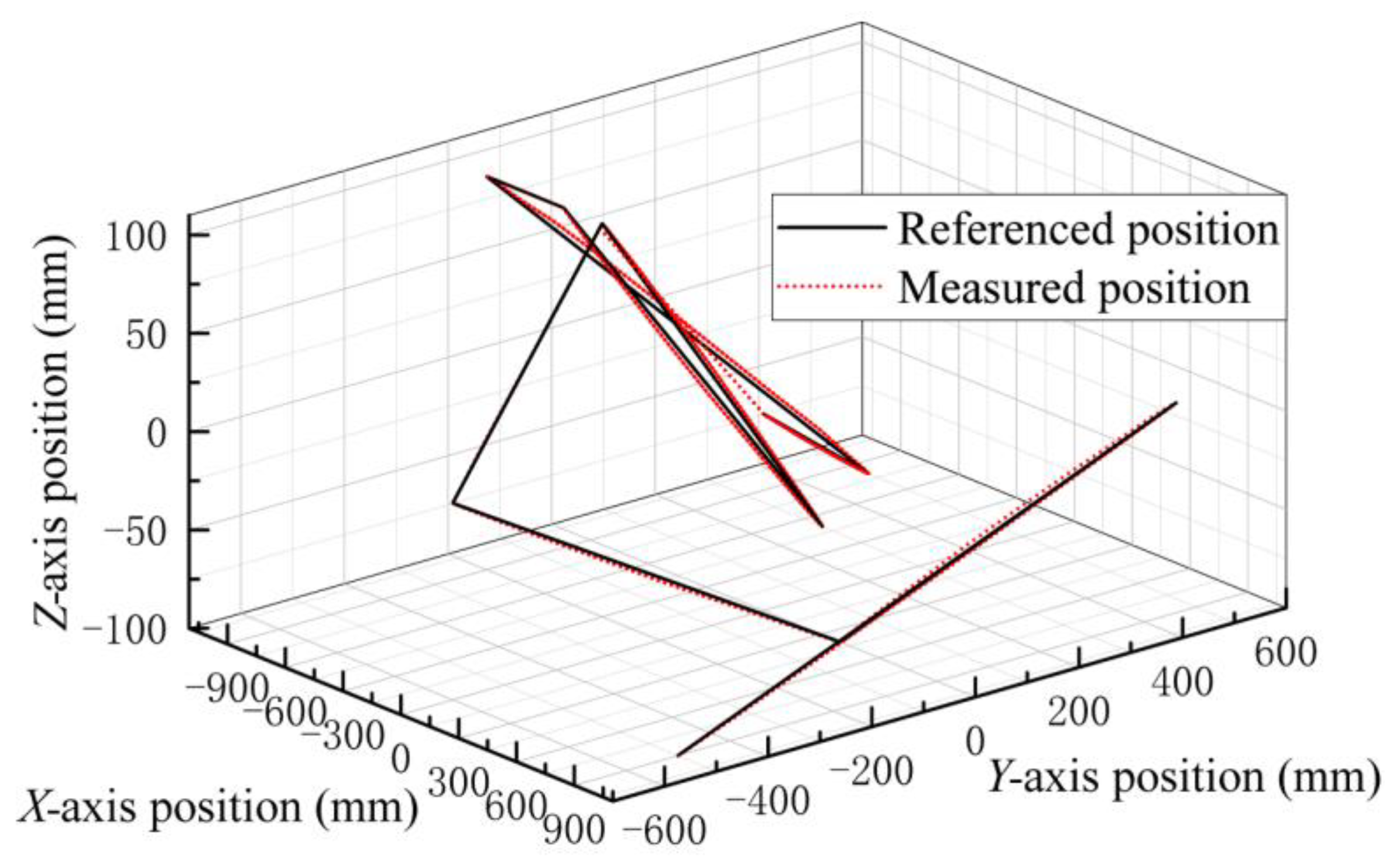
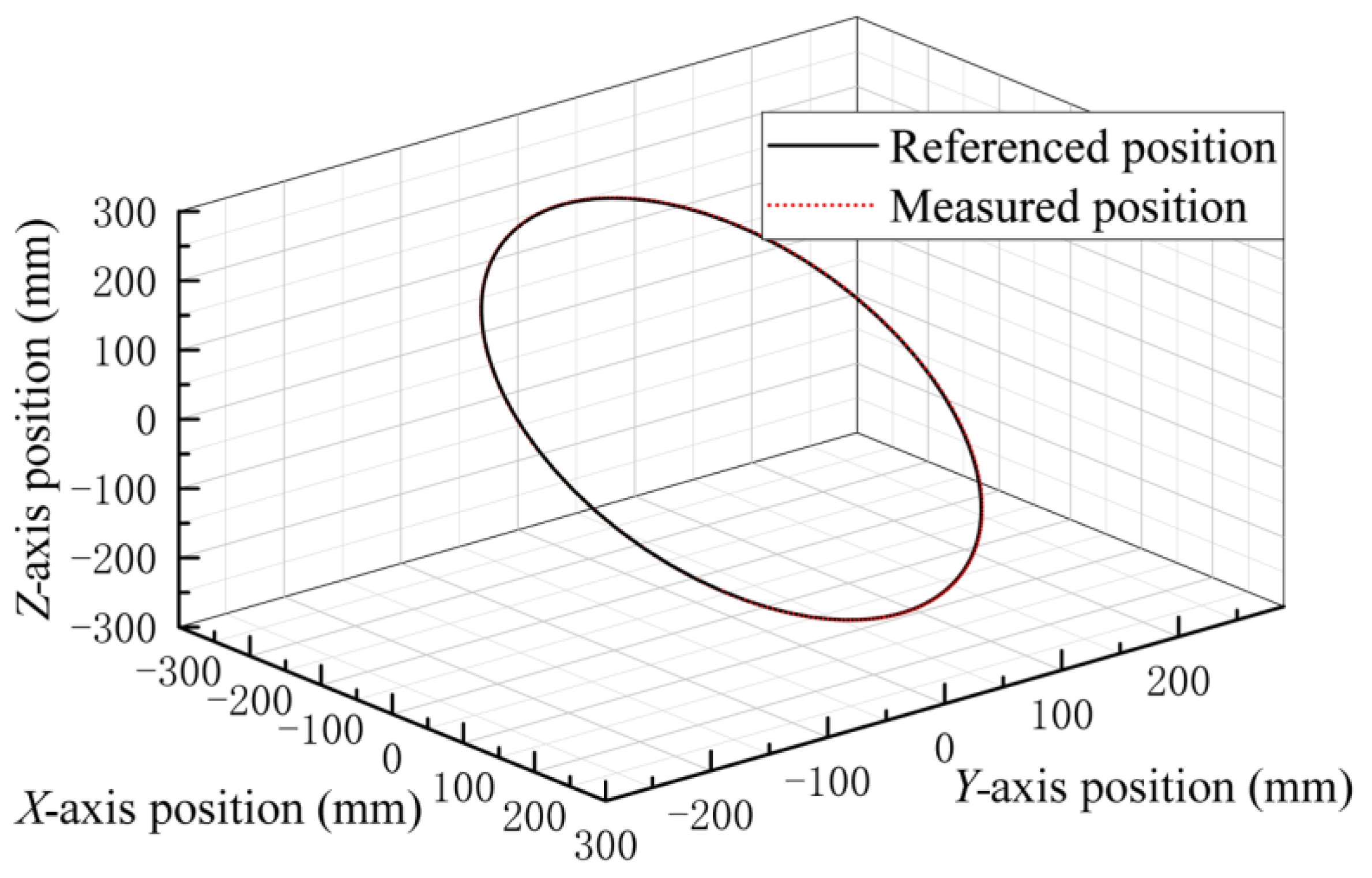
As shown in
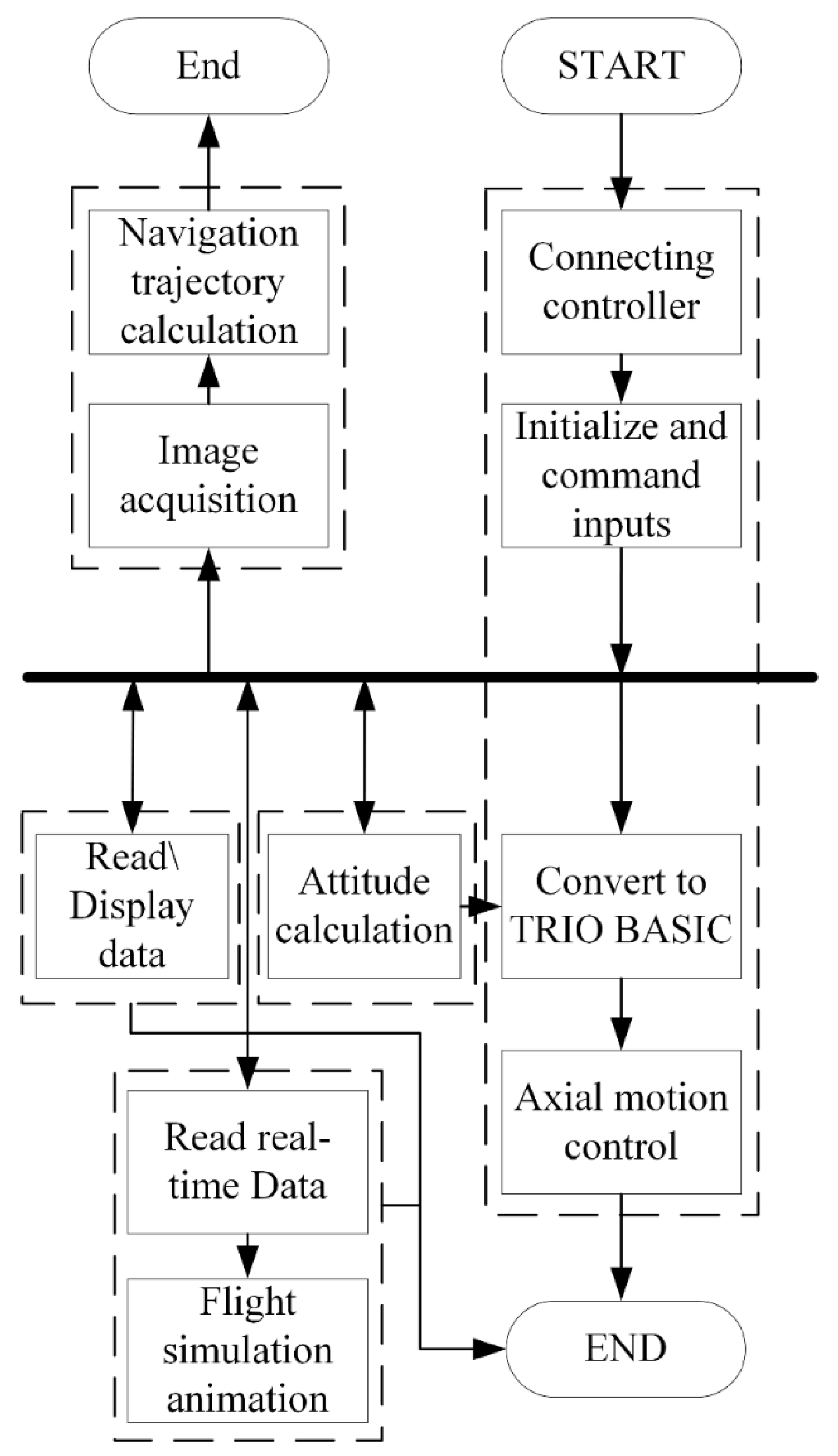
Figure 17 and
Figure 18, a simulated flight trajectory was selected, converted into a TRIO BASIC command and then read to obtain the actual trajectory map. After measurement and calculation, the dynamic error of the three-axis translation table was 0.4 mm.
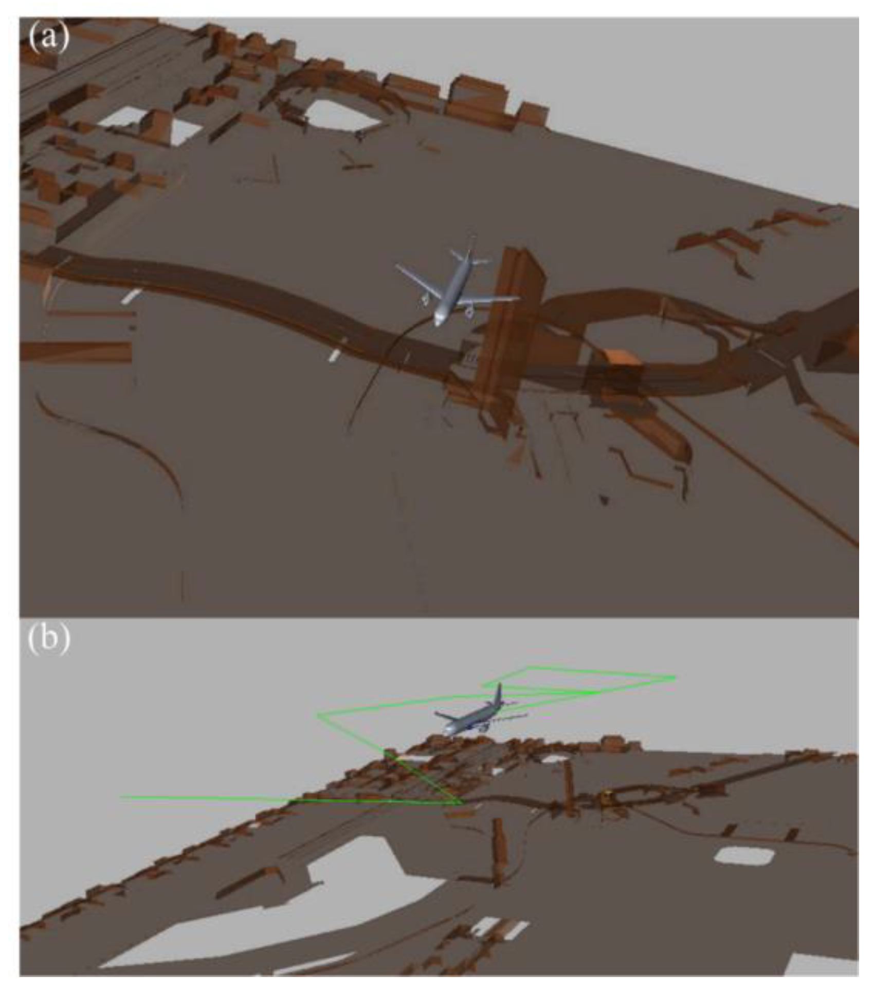
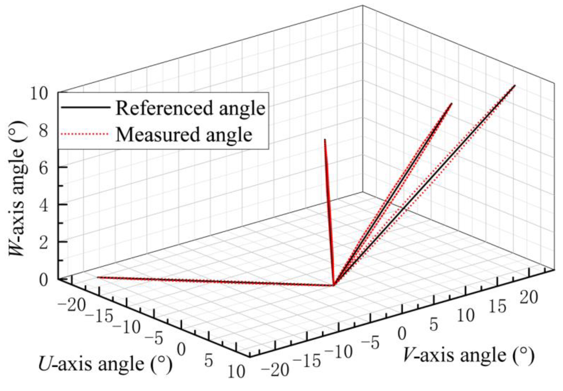
To represent the dynamic-rotation-angle error of the three-axis rotary table more intuitively, the angles of the three axes are represented by three-dimensional spatial coordinates in this paper, as shown in
Figure 19. After measurement and calculation, the dynamic-rotation-angle error of the three-axis rotary table was controlled within 0.04°. Fold lines and spatial arcs were selected as the simulated flight trajectories for the test. The flight trajectory was transformed into control information, and the dynamic error was obtained by comparing the actual trajectory map with the given trajectory map after simulating the flight by the three-axis translation stage.
5.3. Optical-Flow Test
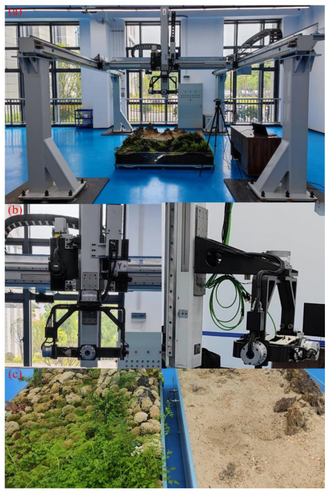
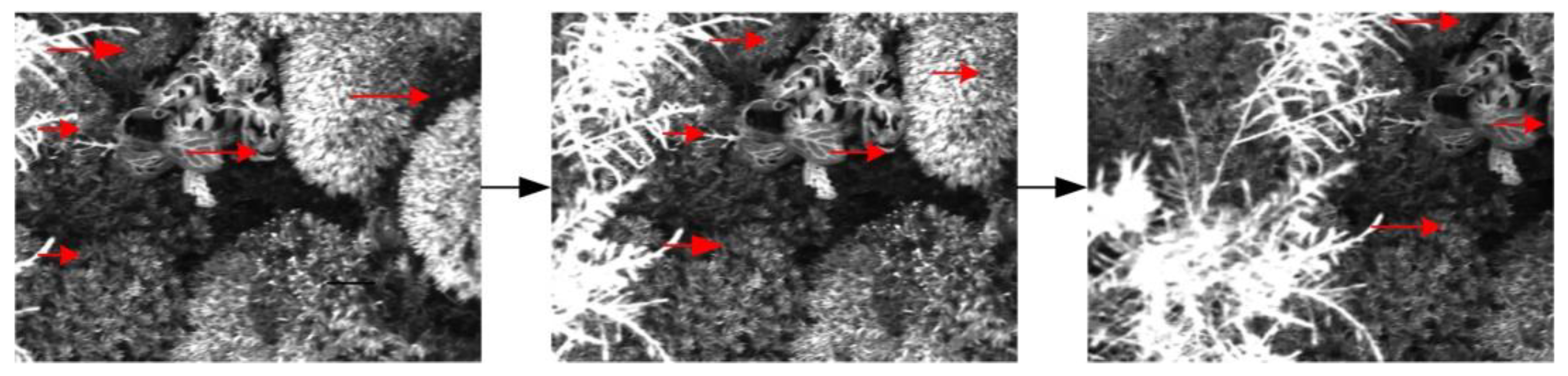
The outdoor flight environment was scaled down and the scenario was replicated in the indoor simulation. Next, the quadrotor UAV simulation system performed the navigation test according to the predetermined trajectory. The end of the simulation system was equipped with an optical detection system, which transmitted the collected optical information to the host computer and calculated the speed using the optical-flow-navigation algorithm. Finally, the trajectory was fitted according to the velocity calculated by the optical flow.
Figure 20 shows the LK optical-flow-calculation results after pretreatment during the indoor flight tests, and its feature points match accurately. The results demonstrate the effectiveness of the simulation platform for testing visual-navigation algorithms.

 ,
, 


