
A Large Neighborhood Search Algorithm with Simulated Annealing and Time Decomposition Strategy for the Aircraft Runway Scheduling Problem

College of Civil Aviation, Nanjing University of Aeronautics and Astronautics, Nanjing 211106, China
*
Author to whom correspondence should be addressed.
Aerospace 2023, 10(2), 177; https://doi.org/10.3390/aerospace10020177
Submission received: 30 November 2022
/
Revised: 31 January 2023
/
Accepted: 7 February 2023
/
Published: 14 February 2023
(This article belongs to the Special Issue Advances in Air Traffic and Airspace Control and Management)
Abstract
:The runway system is more likely to be a bottleneck area for airport operations because it serves as a link between the air routes and airport ground traffic. As a key problem of air traffic flow management, the aircraft runway scheduling problem (ARSP) is of great significance to improve the utilization of runways and reduce aircraft delays. This paper proposes a large neighborhood search algorithm combined with simulated annealing and the receding horizon control strategy (RHC-SALNS) which is used to solve the ARSP. In the framework of simulated annealing, the large neighborhood search process is embedded, including the breaking, reorganization and local search processes. The large neighborhood search process could expand the range of the neighborhood building in the solution space. A receding horizon control strategy is used to divide the original problem into several subproblems to further improve the solving efficiency. The proposed RHC-SALNS algorithm solves the ARSP instances taken from the actual operation data of Wuhan Tianhe Airport. The key parameters of the algorithm were determined by parametric sensitivity analysis. Moreover, the proposed RHC-SALNS is compared with existing algorithms with excellent performance in solving large-scale ARSP, showing that the proposed model and algorithm are correct and efficient. The algorithm achieves better optimization results in solving large-scale problems.
1. Introduction
Air traffic is becoming increasingly congested, due to the relatively fixed airspace capacity. Air traffic throughput is expected to be twice as high as in 2019 by 2040 [1], and aircraft delays are likely to increase further. Airports are the key nodes of the air route network. Improving the operation efficiency of the airport would greatly reduce the delay of the air route network. Airport operations need to meet both aircraft demand and aircraft punctuality rate requirements. The runways are more likely to become the bottlenecks in airport operations, especially in large and busy airports in high demand [2]. To solve the runway congestion problem, the traditional methods to increase the runway capacity include airport renovation and expansion and increasing the number of runways. However, the above methods require a lot of human and material costs and take a long time to implement. The aircraft runway scheduling during the air traffic flow management (ATFM) process can rationalize the runway sequence of departure and arrival aircraft without increasing the infrastructure cost, thus realizing the efficient use of the runway capacity and reducing the related delays.
The aircraft runway scheduling problem (ARSP) is a huge challenge for air traffic management. Runway sequencing is a tactical traffic management technique in which air traffic controllers assign runway use sequences for arrival and departing aircraft. In practice, air traffic controllers often make decisions based on aircraft operations situation in order to resolve conflicts in runway use. While the controller’s own decisions can improve runway utilization efficiency, the limitations of the controller’s own control experience often result in unnecessary aircraft delays during peak hours. Therefore, for the existing airport system, using the limited capacity to optimize aircraft landing and takeoff can scientifically allocate the available runway resources, and effectively reduce aircraft delays and improve airport operational efficiency. In this paper, we design a large neighborhood search algorithm with simulated annealing and time decomposition strategy to solve the ARSP. The effectiveness of the RHC-SALNS algorithm is tested by comparing the actual operation data of Wuhan Tianhe Airport with the existing algorithms with excellent performance in solving large-scale ARSP.
1.1. Problem Description
The classical ARSP can be described as follows: A group of departing aircraft are ready to take off on the airport surface, and a group of arrival aircraft are ready to land. Each departing aircraft has an estimated take-off time window, and each arrival aircraft has an estimated landing time window. According to the aircraft wake turbulence types, runway resources are assigned to each aircraft based on meeting the runway safety separation requirements, i.e., the take-off or landing time of the aircraft. Time deviation cost is incurred when the aircraft assigned runway usage time deviates from the estimated runway usage time. The departure or landing time can be optimized by runway sequencing to reduce the overall time deviation cost [3]. The ARSP covers the airport terminal area, and its structure is schematically shown in Figure 1, where arrival (departure) aircraft enter (leave) the terminal area from different arrival (departure) fixes according to the instrument approach (departure) routes.
The ARSP schematic is shown in Figure 2, where the serial numbers indicate the landing sequence of arrival aircraft or the departure sequence of departure aircraft. For arrival aircraft, the starting adjustment boundary of the landing sequence is generally the boundary of the airport terminal area, and the ending adjustment boundary is generally determined by a key point such as the distance or time point before the specified landing. For departure aircraft, the starting adjustment boundary of the departure sequence is the point at which the aircraft is parking on the apron, and the ending adjustment boundary is the point at which the aircraft is ready to join the departure queue before entering the runway entrance. The area between the starting and ending adjustment boundaries of the runway use sequence is called the aircraft runway scheduling area, i.e., the sequencing algorithm is applied between these two boundaries to schedule the taking off and landing based on information such as expected departure time, expected landing time, and aircraft type [4].
ARSP is the problem of determining the aircraft taking-off or landing sequence by optimizing some specific performance objectives subject to various constraints [5]. ARSP is an NP-hard problem because of the need to consider the differences in the effects of aircraft type (takeoff or landing) and wake turbulence safety separation. At the same time, the scheduling results for ARSP need to meet the requirements of timeliness. ARSP, as a tactical traffic management problem, requires aircraft runway sequencing decisions to be given within a short time frame, thus attracting extensive attention from scholars [6,7]. Aircraft runway scheduling timeliness mainly focuses on the computation time of the algorithm. The scheduling performance needs to meet certain requirements in order to make the algorithm give the runway scheduling results in a certain limited time. In the process of aircraft runway scheduling, in order to find the balance between scheduling efficiency and timeliness, it is often necessary to lose some optimization indices to a certain extent, so that the model solution time can meet the timeliness requirements. Therefore, the main concern of this paper is how to improve the solution efficiency and meet the requirement of ARSP timeliness while ensuring the accuracy of the ARSP solution.
1.2. Literature Review
Relevant scholars have previously carried out research on the ARSP problem, and at present, certain results have been achieved. The research on ARSP can be traced back to 1964, when Ratcliffe [8] elaborated on the runway scheduling concept of first-come-first-served (FCFS), i.e., scheduling aircraft according to their expected landing and taking-off times. Although FCFS can reduce aircraft delays while ensuring relative fairness, FCFS principles may lead to excessive delays for individual aircraft [9], which is not efficient for reducing aircraft delay losses, shortening the total aircraft operation time, and making full use of runway capacity. Therefore, most scholars regard the aircraft runway scheduling of arrival and departure aircraft as a resource allocation problem and use optimization theory to build a model to solve it. The optimization object of the model is the aircraft within the planning time period; the constraints of the model can be categorized and summarized as runway safety separation constraints [10], landing and taking-off time window constraints [11], runway capacity constraints [12], aircraft turnaround time constraints [13], and aircraft priority constraints [14]. The optimization indices of the model are generally aircraft delay time [15], total aircraft operation time [16], and aircraft emission indicators [17,18]. Different combinations of different objectives could produce different optimization results. Generally, ARSP can be formulated as similar problems in other research fields [19]. Carr [9] introduced the traveling salesman problem (TSP) models and Bennell [5] introduced the traveling repairman problem (TRP) models to build the ARSP model. Both of them considered the wake turbulence separation between aircraft and the runway occupancy time as the significant constraints. Beasley [20] and Bertsimas [21] proposed mixed integer programming models (MIP), which treat the aircraft sequence and the time assigned as decision variables and use artificial variables to transform the model into a linear problem. Ceberio [22] introduced the idea of solving the permutation flow shop scheduling problem (PFSP) into ARSP, which deeply integrated ARSP research with practical applications. Balakrishnan [16] treats the sequence of aircraft runway usage as edges in a network and introduces a nodal network model into ARSP. Lieder [23] established a dynamic programming model for runway scheduling of arrival aircraft based on runway state transfer function and runway state transfer cost for different aircraft wake turbulence. As the research progresses, in order to make the ARSP model more applicable to the complex operation environment, scholars have added the winter de-icing operation mode [7], the interactions between runways in complex runway configurations [24,25], and the influence of arrival and departure traffic distribution on controllers’ strategies [26] into the ARSP model to improve the practicality.
With the continuous research on ARSP, the models have gradually matured. The optimization model tends to be more complex, the number of model constraints is increasing, and the model optimization objective function is more refined, which puts forward higher requirements for the solution algorithm of the ARSP model. There are two main types of algorithms for solving ARSP models: exact solving algorithms and heuristic solving algorithms. Traditional exact solution algorithms include the simplex method, dual simplex method, branch-and-bound method, and commercial solvers such as CPLEX and Gurobi. They have been shown to consume a large amount of time in solving large-scale ARSP due to the large solution space [21]. Therefore, many scholars adopt the simplified exact solution algorithm to reduce the size of the solution space, so as to improve the operational efficiency of ARSP. Balakrishnan [16] considered the aircraft as nodes in a network and aircraft runway usage sequences as edges in a network and used node attributes to determine constraints to reduce the size of the solution space. Sölveling [2] improved the branch-and-bound algorithm by defining pruning rules, which can dynamically change the number of samples for estimating the upper and lower bounds during the operation. De Maere [27] studied and proved that the performance of scheduling is only related to the wake turbulence separation of different aircraft types, so the pruning rule of aircraft scheduling was proposed to keep the original order of aircraft with the same wake turbulence separation. This pruning method can reduce the size of the solution space and reduce the computing time of the exact algorithm. Maximilian [7] combined constraint programming (CP) with a column generation algorithm to further reduce the solution space. Usually, heuristic algorithm solving can quickly obtain feasible solutions with high quality. Using heuristic algorithms to solve large-scale ARSP can shorten the solution time and improve computing efficiency while ensuring the solution accuracy. Heuristic algorithms for solving ARSP problems include genetic algorithms [28], simulated annealing algorithms [29], ant colony algorithms [30], etc. We were also motivated by the fact that meta-heuristic frameworks are very adaptable, enabling other meta-heuristic algorithms to be easily hybridized with them. Salehipour [31] combined a variable neighborhood search algorithm with a simulated annealing algorithm. The ARSP is initially solved using the genetic algorithm, and the aircraft sequence was fine-tuned under the constraints until the termination condition of the algorithm is met. Sabar [32] developed the iterated local search (ILS) algorithm, which avoids the algorithm to compute results into local optima by defining perturbation operators. In the same year, Shihao Wang [33] added a linear differential decreasing annealing strategy to the traditional simulated annealing particle swarm algorithm (SA-PSO) to solve the problems of slow convergence speed. In 2019, Liu Qi [34] proposed the STW-GA dynamic algorithm by combining the sliding time window algorithm with the dual-structured chromosome genetic algorithm, which can ensure the fairness of aircraft scheduling while reducing the total delay time. Junfeng Zhang [35] developed a multi-objective imperial competition algorithm to solve the arrival aircraft scheduling problem. In 2021, Lily Wang [36] combined the sliding time window algorithm with the particle swarm optimization algorithm to develop a combined TW-PSO algorithm, which obtained better optimization results while reducing the number of iterations of the algorithm.
We also note that the time decomposition strategy can divide the large-scale problem into several subproblems for solving to achieve the optimal solution [37]. Among them, the receding horizon Control (RHC) strategy has been shown to be a very effective optimization strategy for large-scale optimization problems with complex constraints [13]. In the RHC strategy framework, the original optimization problem is partitioned into several subproblems, thus increasing the problem solution rate. Hu [38] established a dynamic arrival aircraft scheduling model based on the RHC. The arrival aircraft scheduling model has good robustness, and the RHC strategy can achieve an optimal solution quickly. Using the RHC strategy to make relevant decisions is required to look forward to multiple time horizons. When optimizing the current time horizon, the aircraft information is optimally scheduled forward over multiple time horizons, but only the results are implemented on the current horizon and the same process is repeated on the next horizon. Clarke [39] combined the RHC strategy with predictive techniques to update each piece of operational information of aircraft in real time to recalculate the uncertainty delays every 15 min. Kjenstad [13] applied the RHC strategy by dividing the length of time horizon into 10-to-15 min and adjusting the number of time horizons to find a combination of parameters with fast speed and high accuracy. The feature that the RHC framework is more adaptable also draws our attention, and it can hybridize with other heuristic strategies to improve the efficiency of the problem solving. For example, Qiqian Zhang [40] combined the RHC strategy with a genetic algorithm (RHC-GA) to guarantee the solution quality and improve the solving speed.
The above-mentioned literature contain information regarding some preliminary research conducted on the ARSP model and solution algorithm and achieved great research results. It should be noted that the research on the ARSP model has been gradually sophisticated, which makes the model can be increasingly used in a wide range of applications. However, the corresponding solution algorithms do not achieve the purpose of solving the model quickly, accurately, and efficiently. The corresponding solution algorithm cannot give optimal solution results in a short time frame due to the large solution space and excessive complexity. Although some of the aforementioned works deal with improving the algorithmic solution efficiency of ARSP, the overview shows that most of the studies enhance the solution efficiency of ARSP with a single heuristic strategy, while few of them investigate the advantages of frameworks that combine multiple heuristic strategies. Regarding the solution algorithm, we believe that the advantages of various heuristic strategies should be combined to meet the decision-making needs of airports, air traffic controllers, and airlines in practice. To this end, the main contributions of this paper are the following two points:
- (1)
- This research aims to improve the neighborhood construction method, which is one of the cores of the simulated annealing algorithm. We propose the large neighborhood search simulated annealing algorithm (SALNS). The breaking process, reorganization process, and local search process are introduced to improve the efficiency of the algorithm operations. Combining the large neighborhood search with a simulated annealing algorithm can fully utilize the advantages of both.
- (2)
- We aim to combine the RHC framework with the SALNS algorithm, and propose the RHC-SALNS algorithm to further improve the efficiency of the algorithm for solving ARSP models.
1.3. Organisation of the Paper
The remainder of this paper is organized as follows: Section 2 introduces an optimal scheduling model for ARSP. Section 3 explains the calculation process and critical steps of the algorithm. In Section 4, the instances of Wuhan Tianhe Airport are used to demonstrate the effectiveness of our proposed algorithm. Section 5 discusses the conclusions.
2. Mathematical Model
We investigate an ARSP model that considers both arrival aircraft and departure aircraft, aiming to improve the performance by reducing weighted aircraft delays. It is important to note that airports with multiple runway configurations are widely available in China, and at the same time, the runway operation mode of independent parallel operation is the development trend of Chinese airports. In this paper, we chose a public runway configuration with independent parallel operation (04L|22R) at Wuhan Tianhe Airport for analysis. The assumptions for the ARSP are outlined below.
Assumption 1.
The uncertainty factor of aircraft operation is not considered; the runway configuration and operating mode will not change during the ARSP planning time period.
Assumption 2.
The operations of multiple runways are independent; the aircraft takeoff and landing operations are not affected by the aircraft of other runways.
Assumption 3.
For each combination of runway and parking position at the airport ground area, there will be a pre-determined transition path between them.
2.1. Notations
To ensure the lowest aircraft delays, the runway scheduling optimization model for arrival and departure aircraft, based on the concept proposed by Bertsimas [21] and Hancerliogullari [3], , is the set of aircraft that requiring scheduled during the planning time period, where ; is a set of arrival aircraft that land at the airport and stay until planning time period; is a set of arriving–departing aircraft that arrive at the airport and depart from it after a turnaround duration, i.e., the aircraft have continuous consecutive voyage at this airport; is a set of departing aircraft that is parked at the airport at the beginning of the planning time period and depart later. In order to simplify the descriptions, we divide the set into two sets, where denotes the set of arrival aircraft in the set and denotes the set of aircraft in the set: . For aircraft during the planning period, we sort their expected runway usage time in ascending order, i.e., for , aircraft are first sorted by comparing their (for arrival) and (for departure). As an example, if , , then . In this paper, the runway operation mode is an independent parallel operation mode. The two runways can be considered as two independent single runway systems, where the taking-off and landing operations on the runways do not affect each other. Therefore, in our ARSP model, we will focus on the aircraft runway assignment variables [41,42], as well as the landing time and taking-off time assignment variables.
Additionally, many current studies ignore the process of aircraft turnaround operations, also referred to aircraft ground handling. In this paper, we consider the minimum turnaround separations, which are defined as the time required to unload the aircraft after its arrival at the gate and to prepare it for departure again.
The relevant sets, parameters, and variables required for the model are shown in Table 1.
2.2. Constraints
2.2.1. Safety Separation Constraints
For aircraft using the same runway, minimum separation requirements must be met to comply with the safety regulations implemented by the Federal Aviation Administration (FAA) and the International Civil Aviation Organization (ICAO) [43,44], as shown in Equation (1). There is one and only one sequence of any two aircraft using the runway, as shown in Equation (2). Each aircraft can only use one runway, as shown in Equation (3).
2.2.2. Time Window Constraints
The landing time assigned to each arrival aircraft must be within the time window defined by the expected landing time and the maximum acceptable delay, as shown in Equation (4). The take-off time assigned to each departing aircraft must be within the time window defined by the expected take-off time and the maximum acceptable delay, as shown in Equation (5).
2.2.3. Runway Occupancy Time Constraints
Each runway can only be occupied by one aircraft at the same time. For aircraft using the same runway continuously, the runway use separation is the greater of and . For medium-sized aircraft, will generally be greater than .
2.2.4. Flight Turnaround Constraint
Let departing aircraft and arrival aircraft be a pair of connected aircraft, that is to say, arrival aircraft will be pushed back from the gate by the identification of departing aircraft after the turnaround process of . Then, the difference between the assigned take-off time of departing aircraft and the assigned landing time of arrival aircraft must be larger than the minimum connection coefficient .
2.3. Objectives
Minimum weighted aircraft delays:
where . is the weight of arrival aircraft delay. If the aircraft is speeded up before its arrival, the actual runway time will be earlier than the estimated runway time. Here, we define the negative delay as “gray delay”, meaning that the assigned time is ahead of the estimated time. Note that, in order to ensure flight punctuality as much as possible, the negative delays in the presence of time advance of arrival are also counted as delays in terms of absolute value. Since advanced or delayed operations are not symmetrical in their performance effect, the values should be set according to the actual operation of the airport. In the case of this paper, by investigating the actual operation of the airport, when “gray delay” occurs and when delay occurs. is the delay cost factor of aircraft, where . is the priority factor of aircraft . is the maximum value in the priority table, as shown in Table 2. The three dimensional priority table is designed to reflect the scheduling priority factors. Specifically, for each aircraft , the corresponding characteristic parameters of voyage consecutiveness, aircraft type, and arrival or departing aircraft are denoted as , , and , respectively. Aircraft scheduling should not only consider the current aircraft, but also whether it will affect the next departing aircraft, with consecutive voyages at this airport. The aircraft with consecutive voyages should be given a higher priority. Second, the type of aircraft reflects the number of seats guaranteed, and empirically, a higher priority is generally given to larger aircraft types. It is worth noting that we consider the overall performance of airside traffic management. We consider the arrival (departing) peaks of airport operations. The higher priority on arrival (departing) peaks will be given to the arrival (departing) aircraft. The specific, detailed description of the priorities refers to the literature [45]. The values of each parameter are shown as follows:
The priority factor of the aircraft can be calculated as follows:
where .
| the voyage of aircraft i is consecutive | |
| otherwise | |
| the type of aircraft i is super | |
| the type of aircraft i is heavy | |
| the type of aircraft i is medium | |
| the type of aircraft i is light | |
| i is an arrival (departing) aircraft at airport arrival (departing) peaks | |
| otherwise |
Taking a light aircraft with inconsecutive voyages and which does not at peak hours as an example, i.e., , , the priority of the aircraft is . Similarly, the priority of each aircraft can be obtained as shown in Table 2.
3. The Proposed Method
In this paper, a large neighborhood search algorithm with simulated annealing and receding horizon control strategy (RHC-SALNS) is proposed for solving ARSP. The simulated annealing algorithm is a simulation of the physical process of the high temperature annealing of a solid material, in which a solid material is heated to a high enough temperature and then cooled down gradually. During the warming process, the internal energy of the solid material is large and the internal particles become disordered. As the temperature decreases, the internal energy decreases and the internal particles become stable and can reach equilibrium at each temperature. The internal energy is reduced to a minimum when the temperature of the object drops to a certain base-state temperature. The simulated annealing algorithm exploits the similarity between combinatorial optimization and physical annealing processes to find the global optimal solution in the solution space by combining the probabilistic sudden jump property. In this paper, we use the simulated annealing algorithm framework to design a large neighborhood search method to replace the original neighborhood construction method. The breaking, reorganization, and local search processes were proposed to form a new solution.
3.1. Algorithm Design
In the RHC strategy framework, the original optimization problem is partitioned into several subproblems to improve the solving rate. The RHC strategy framework has been widely studied and matured by scholars [37,38]. The RHC strategy algorithm is described in detail in Section 3.5. The SALNS algorithm is used to optimize runway scheduling for aircraft on each time horizon. The flowchart of our proposed RHC-SALNS algorithm is shown in Figure 3. The simulated annealing (SA) algorithm was first proposed by Steinbrunn [46]. It is a general optimization algorithm with better solution results than other heuristics and has the advantage of being insensitive to the initial parameter settings. However, as a type of heuristic algorithm, simulated annealing algorithms are also prone to falling into the local optimal solution. The SALNS algorithm uses the simulated annealing algorithm framework to generate the algorithm parameters and initialize the initial solution. The algorithm uses a large neighborhood search to construct neighborhood solutions in the process of generating new solutions. The algorithm accepts the neighborhood solution by calculating the objective function value using the Metropolis criterion [46] until the stop condition is satisfied. The specific steps of the RHC-SALNS algorithm are as follows.
- Step 1: Initialize the algorithm initial temperature , algorithm termination temperature , cooling coefficient , number of internal cycles , number of non-updating generations , and maximum number of non-updating generations ; encode and generate the initial solution (see Section 3.2, Section 3.3 for details), and then .
- Step 2: Calculate the objective function value of the current initial solution and make the optimal solution , and the optimal solution objective function value is .
- Step 3: If , execute Step 4; otherwise, make and execute Step 7.
- Step 4: The initial solution is broken (see Section 3.4.1 for details), reorganized (see Section 3.4.2 for details), and locally searched (see Section 3.4.3 for details) to generate the neighborhood solution .
- Step 5: Calculate the objective function value of the neighborhood solution ; accept the neighborhood solution according to the Metropolis criterion, .
- Step 6: If , then make , , , and return to Step 3.
- Step 7: . If the solution under the current temperature is the same as the solution under previous temperature, then .
- Step 8: If , or , stop the algorithm and output the optimal solution and the objective function value ; otherwise, return to Step 3.
3.2. Code
We use the real number encoding method. In the planning period, there are aircraft with the number and runways with the number , where the aircraft were numbered and sequenced in the ascending order proposed in Section 2.1. Figure 4 shows the solution representation code of 10 aircraft of two runways, where 11, 12 represent runway 04 and 22L, respectively, and the code shown in Figure 4 can be converted into the aircraft sequence of runway 04: ; the aircraft sequence of runway 22L is .
3.3. Initialisation
The algorithm needs to generate the initial solution of the aircraft runway sequence in the initialization process. In the initialization process, a first-come-first-served greedy random initialization method is used to ensure the diversity of the initial solution due to the high efficiency of the large neighborhood search method proposed in this paper. The greedy random initialization could reduce the complexity, which can further improve the efficiency of the algorithm. The specific steps of greedy random initialization are as follows.
- Step 1: Randomly distribute the aircraft to all runways.
- Step 2: Based on the runway allocation result of Step 1, the aircraft sequence of each runway is initialized to first-come-first-served. Take one of the runways as an example; select the aircraft with the smallest expected runway usage time as the first to use that runway.
- Step 3: The aircraft that is closest to the last assigned aircraft in terms of runway usage time is not scheduled as the next aircraft to use the runway. Repeat until all the aircraft are scheduled.
- Step 4: Based on the generated aircraft sequence above, the runway usage time of the aircraft is assigned according to the constraints in Section 2.2.
Algorithm 1 shows the pseudo-code of the initial solution generation method.
| Algorithm 1. Initial solution generation method |
| be the number of aircraft and be the number of runways; |
| be the safety separation between aircraft and aircraft ; |
| 3: Set The solution after the breaking and reorganization process; |
| 4: Sort the aircraft based on their estimated runway usage times , and add them to , where |
| 5: while do |
| 6: Randomly select a runway from and add to ; |
| 7: ; |
| 8: end while |
| 9: while do |
| 10: for each two aircraft and belong to |
| 11: If then assign to ; |
| 12: Else assign to ; |
| 13: end if |
| 14: ; |
| 15: end while |
| 16: Return the generated solution |
3.4. Large Neighborhood Search
The large neighborhood search consists of three main processes—the breaking process, reorganization process, and local search process—which are implemented sequentially for the current solution when constructing the neighborhood solution. The breaking and reorganization processes are able to search within a large structure of the solution space, and thus have a higher probability of finding the optimal solution compared to the other traditional methods. In addition, the complexity of the algorithm is reduced due to the simpler greedy random insertion method in the reorganization process, which balances the efficiency and effectiveness of the large neighborhood search process. After obtaining the initial solution of the greedy randomized algorithm, the large neighborhood search can effectively find the optimal solution or the near-optimal solution. The large neighborhood search process is shown in Figure 5.
3.4.1. Breaking Process
The breaking process of the solution consists of four types of methods, namely, adjacent breaking (), maximum saving breaking (), random breaking (), and single point breaking (). During the execution of the breaking process, are executed sequentially, and the broken aircraft are stored in the insert array for reorganization.
The specific steps of each breaking method are as follows:
adjacent breaking.
- Step 1: Select a random aircraft as the root.
- Step 2: Calculate the maximum number of removed aircraft , , where ⌈ ⌉ denotes upward rounding and is the probability of adjacent breaking.
- Step 3: Randomly select the number of aircraft , is a random number between .
- Step 4: Remove the root aircraft and the closest aircraft from the root aircraft from the original sequence and add them to the Insert array.
maximum saving breaking.
- Step 1: Calculate the cost of aircraft delay savings for each aircraft after it is removed from the aircraft queue: , .
- Step 2: Calculate the maximum number of removed aircraft , , where ⌈ ⌉ denotes upward rounding and is the probability of maximum saving breaking.
- Step 3: Randomly select the number of removed aircraft , is a random number between .
- Step 4: Randomly select aircraft according to the roulette method, where the larger the , the greater the chance of the aircraft being selected for removal. Then, removal the selected Q2 aircraft to the insert array.
random breaking.
- Step 1: Calculate the maximum number of removed aircraft , , where ⌈ ⌉ denotes upward rounding and is the probability of random breaking.
- Step 2: Randomly select the number of removed aircraft , is a random number between .
- Step 3: Randomly select aircraft, remove all the selected aircraft, and add them to the insert array.
single point breaking.
- Step 1: Generate a random number between .
- Step 2: If , then randomly remove an aircraft from the aircraft sequence and add it to the insert array. is the single point breaking probability.
The proposed breaking process is presented in Algorithm 2.
| Algorithm 2. Breaking process |
| 1: Let be the number of the proposed breaking process; |
| 2: ; |
| 3: The solution after the initial solution generation process; |
| 4: while do |
| 5: Performs the initial solution breaking process using ; |
| 6: Put the breaking aircraft into the Insert array |
| 7: ; |
| 8: end while |
| 9: and Insert array |
3.4.2. Reorganization Process
All removed aircraft are reinserted into the aircraft runway sequence during the reorganization process. The aircraft will be placed in random order and greedily randomly inserted into the runway sequence. The specific reorganization steps are as follows.
- Step 1: Randomly disorder the aircraft to be inserted in the Insert array.
- Step 2: If there is no point to be inserted, end; otherwise, find the aircraft positions available for insertion on each runway according to the aircraft runway usage time constraint in Section 2.2.
- Step 3: Calculate the increase in cost for all positions available for insertion, randomly select the position with the smallest or second smallest cost, and return to Step 2.
The proposed reorganization process is presented in Algorithm 3.
| Algorithm 3. Reorganization process |
| 1: Let be the number of the breaking aircraft; |
| 2: The solution after the breaking process; |
| 3: Randomly disrupt the aircraft in the insert array; |
| 4: while do |
| 5: the positions on each runway available for aircraft according to the safety interval and the time window constraint in Section 2.2; |
| 6: Calculate the insertion cost of each insertable point and sort them in ascending order |
| 7: Randomly insert the aircraft at the insertion point and ; |
| 8: ; |
| 9: end while |
| 10: Return as |
3.4.3. Local Search Process
The local search process contains four steps, namely, . and try to change the runway usage time of the aircraft; and try to change the runway of the aircraft. When the aircraft runway scheduling solution goes through the process of destruction and reorganization, four local search processes are executed sequentially. If a better solution appears, the current step is repeated until no better solution is produced [32].
means to perform a binomial swap on the aircraft queue of the same runway, randomly select a runway, select two aircraft in this aircraft queue, swap the sequence of aircraft located between two aircraft in the aircraft queue under the constraints, check all possible swaps between these aircraft, generate a new aircraft runway queue, calculate the new objective function value, and keep the current solution if the objective function value decreases.
means to conduct a binomial swap of aircraft sequence of different runways, randomly select a runway, select two aircraft in this aircraft queue, select the closest time between the two aircraft in the other runway queue, swap the aircraft that are located between the two aircraft with the aircraft located between the two aircraft in the other runway queue under the constraints, calculate the new objective function value, and keep the current operation if the objective function value decreases.
means to transform the aircraft sequence of the same runway, randomly select a runway, check all aircraft on that runway and insert them before or after the aircraft with the closest runway usage time, generate a new aircraft runway queue, calculate a new objective function value, and keep the current solution if the objective function value decreases.
means to transform the aircraft sequence of different runways, randomly select a runway, check all aircraft on that runway and insert them before or after the aircraft on different runways with the closest distance to their runway usage time, generate a new aircraft runway queue, calculate a new objective function value, and keep the current solution if the objective function value decreases.
The proposed local search process is presented in Algorithm 4.
| Algorithm 4. Local search process |
| 1: Let be the number of the local search process; |
| 2: Set ; |
| 3: The solution after the breaking and reorganization process; |
| 4: while do |
| 5: Generates a neighborhood of using ; |
| 6: If then |
| 7: ; |
| 8: ; |
| 9: else |
| 10: ; |
| 11: end if |
| 12: end while |
| 13: Return |
3.5. Time Decomposition Approach
During actual airport operations, air transport decision makers are primarily concerned about the efficiency of solving the ARSP model. Therefore, the computation time of the algorithm is critical. A hybrid algorithm combining heuristic methods and accurate algorithms may have more potential than traditional heuristics or accurate algorithms for the complexity of the problem [47]. Therefore, we propose an algorithm combining RHC strategy and SALNS to solve the ARSP model.
Receding horizon control strategy has been shown to be an effective optimization strategy for large-scale optimization problems with complex constraints [48]. In the RHC strategy framework, the original optimization problem is partitioned into several subproblems. The RHC strategy is required to look forward time horizons, i.e., when optimizing the current kth time window, the optimal scheduling looks forward C time horizons, but only implements the results in the kth horizon and repeats the same process on the next optimization stage. We give the specific procedure of the RHC-SALNS in the following.
3.5.1. Aircraft Status Classification
In order to determine the aircraft involved in a given time horizon, we propose a classification rule for the aircraft status. For each aircraft, the status is assigned based on the earliest landing time/taking-off time and the scheduled landing time/ taking-off time. The necessary parameters to determine the aircraft status include:
is the length of an operating interval.
is the length of receding horizon.
denotes the beginning time of the receding horizon at the kth operating interval; the operating time interval is when the optimization scheduling is at the kth stage.
denotes the scheduled runway usage time of aircraft is in the interval after the kth optimization scheduling stage.
Suppose that we optimize the horizon; the aircraft will be classified and marked with a status according to the following rule:
Completed aircraft: : this status means that the aircraft has been optimized in a previous horizon and has no interaction with the aircraft that need to be optimized in the current horizon.
Ongoing aircraft: : this status means that the aircraft has been optimized in the previous horizon, but it will be still interacting with aircraft that need to be optimized. Aircraft of this status also need to be optimized because their decision variables are not fixed.
Active aircraft: : this status means that, as the horizon slides afterward, the planned aircraft will go through the statuses from active to ongoing and then completed.
Planned aircraft: this status means that as the time window receding backwards, the planned aircraft will go through the statuses from active to ongoing and then completed.
3.5.2. Receding Horizon Control Strategy
Before we describe the proposed RHC-SALNS algorithm, some notations are introduced: is the set of aircraft participating in the optimization scheduling of the stage. is the set of aircraft that have completed scheduling after the completion of the kth optimization scheduling stage. is the set of aircraft that have not completed scheduling after the completion of the kth optimization scheduling stage. is the set of aircraft that or in interval . is the weighted sum of the delay time of aircraft that completed scheduling in the kth optimization scheduling stage. For each aircraft, : denotes the estimated take-off time at the kth operating stage. For each aircraft, : denotes the estimated landing time at the kth operating stage. The sets, parameters, state of each aircraft, and the position of the receding time horizons are shown in Figure 6.
- Step 1: Generate the initial aircraft queue in the order of the values of and ; set the of the first aircraft to if the first aircraft ; set the of the first aircraft to if the first aircraft . Let = 0; set the value of ; initialize , , and .
- Step 2: After the completion of the stage of aircraft scheduling, those aircraft with are put into the set . is calculated with reference to Equation (10).Freeze the existing scheduling results of those aircraft with, put them into the set , and update the constraints with reference to Equation (11).Let . Put the aircraft which is in into . Put the aircraft which is in into .
- Step 3: The aircraft that, in , is optimally scheduled in the stage using the SALNS algorithm with reference to Equation (12), where
- Step 4: Let ; if , go to Step 5. Otherwise, go to Step 2.
- Step 5: Calculate with reference to Equation (13).
The proposed RHC-SALNS is presented in Algorithm 5.
| Algorithm 5. RHC-SALNS |
| Require: matrix, , for aircraft its , maximum acceptable delay time . For aircraft its , maximum acceptable delay time . 1: Generate initial parameter value, set , 2: , ; 3: while do 4: use SALNS algorithm schedule aircraft runway operation 5: set choose from which 6: 7: calculate 8: 9: set choose from which 10: 11: for in 12: reset constraints ; 13: end for 14: set choose from which 15: 16: set choose from which 17: 18: set ; 19: ; 20: end while 21: |
4. Experimental Results and Comparisons
In this section, the actual operational data of Wuhan Tianhe Airport in 2020 are used to evaluate the performance of the proposed RHC-SALNS algorithm for the ARSP. For the key parameters in the RHC-SALNS, we performed a parameter sensitivity analysis to determine the optimal combination of parameters. Additionally, we verified the effectiveness of using the time decomposition strategy in improving the efficiency. In further experiments, the algorithm computational results are compared with other algorithms (STW-GA, RHC-GA, TW-PSO, SA-PSO, and ILS).
4.1. Experimental Setup
This section discusses the instances that have been used to evaluate the proposed RHC-SALNS and the parameter settings.
To investigate the performance RHC-SALNS, we run our proposed algorithm with ARSP scenarios of different sizes, different planning durations, and different numbers of aircraft. We use four instances of ARSP at Wuhan Tianhe Airport for our case study. The main characteristics of these instances are shown in Table 3.
In the four instances, the percentage of wake turbulence categories and arrival/departure properties is shown in Figure 7.
The RHC-SALNS was coded in MATLAB R2016a and run on a PC with Intel i7-9700KF8C8T, 3.60 GHz, and 16.0 GB RAM.
4.2. SALNS Parameters Sensitivity Analysis
This section evaluates the proposed RHC-SALNS and the parameter settings. The proposed RHC-SALNS algorithm has many parameters that need to be determined in advance, including the length of the time horizon and the number of receding horizons in the RHC framework, the number of internal cycles in the simulated annealing framework, and the probability of the breaking process in the large neighborhood search algorithm. Please take note that in this section, only the values of the parameters in the neighborhood search component (breaking process) and the simulated annealing framework are properly combined; the parameters for RHC are discussed in Section 4.3. In order to determine the better parameters, we determined the values of all parameters one by one by manually changing the value of one parameter while fixing the values of the other parameters, which are set to the default values. The default values of these five parameters () are 500, 0.2, 0.5, 0.3, and 0.4, respectively. If we obtain an expectation value, it will be applied in the next experiments for sensitivity analysis. Then, the best values of all parameters are recorded. In this process, we randomly select an instance to perform the parameter sensitivity analysis. The instance used is Instance 2. In addition to the above parameters, other parameters throughout our experiments were set as follows: initial temperature , termination temperature , cooling coefficient , maximum number of non-updating generations , , .
During the sensitivity analysis, indices (i.e., the sum of weighted aircraft delays) are recorded to assess performance. To calculate these indices for the sensitivity analysis, we performed more than 30 experiments with default parameters, recording the minimum value of the objective function as the default optimal solution. We conducted 30 separate independent experiments with different combinations of parameters and represent the resulting data distribution in box plot format [49]. Details of the values of the weighted sum of delay time and deviation over 30 independent runs and comparisons between different parameter settings are given in Figure 8 and Figure 9.
In order to find the optimal combination of parameters for the algorithm, we used the Wilcoxon rank sum test [50] to analyse whether the computational results with different parameters are significantly different (with a 5% significant level). Figure 8 and Figure 9 show the p-values under different parameters. It can be seen that for the breaking probabilities , there is no significant difference in the calculated results under each combination of parameters. For , we can find that, when , with the continues increasing of , there is no significant difference in the algorithm calculation results under each parameter, so the parameter of should be chosen. Similarly, we should choose for the choice of parameter . The SALNS algorithm parameters we use in the following calculation process are set in Table 4.
4.3. Receding Horizon Control Analysis
It has been demonstrated that the performance of the adopted RHC strategy is closely related to its key parameters and [13]. , as well as need to be analyzed according to the corresponding problem. Based on the conclusions related to Section 4.2, we use the parameters of Table 4 for our analysis. We randomly select Instance 2, Instance 3, and Instance 4 to analyze the experimental results. The length of the time horizon is set to 30 and 15 min, respectively. The number of receding horizons is set to 2 and 3, respectively. Then, the aircraft within each time horizon are scheduled optimally using the SALNS algorithm. We compared the optimization results and computation time with different combinations of parameters in Table 5. We have bolded the fastest solution time and the optimal objective function value for each instance in Table 6. We can note that the larger the receding horizon or the number of receding horizons , the longer the solution time of the algorithm; however, the results are not necessarily better. Although the choice of parameters influences the objective function values, the differences are small. For example, for Instance 4, the optimal value of and is only 1.15% larger than that of and , but the operation time is reduced by 46.7%. Therefore, considering the actual application, the decision maker can choose the combination of parameters suitable for the actual scheduling scenario by considering the algorithm solution time and the solution result. We also note that the RHC-SALNS algorithm solves significantly better than the SALNS algorithm, improving the objective values by 14.8%, 12.7%, and 10.74% with the optimal objective parameter settings. This is due to the significantly sped up computation time of the RHC-SALNS algorithm, which can find better solutions within the specified time frame. Numerous experiments have shown that the runtime of the scheduled formulation can generally be controlled within 6 s/aircraft [51]. Therefore, the RHC-SALNS algorithm can meet the demand for aircraft operation scheduling decisions at the tactical level.
Meanwhile, we add the computational results of SALNS algorithm without RHC strategy for comparison, as shown in Table 5. Take the case of and for Instance 2 as an example, the number of aircraft with different statuses over 12 horizons are counted as shown in Figure 10. Similarly, take the case of and as an example; the performance of objectives in each time horizon during the RHC-SALNS evolution in 12 horizons are plotted as shown in Figure 11. The values of the objective function in each planning period and solution time for each instance are shown in Table 6.
From the statistics of aircraft status, as shown in Figure 10, we find that, in the first receding horizon, all aircraft in the planning period are active aircraft. However, as the horizon is receding backward, the unplanned aircraft from the previous period are accumulated in the planning time period. This is because, considering the runway separation constraint of between aircraft, a number of aircraft will be delayed during the peak hours, resulting in them not being able to complete the scheduling within the planning time.
It can be shown that the SALNS algorithm completes convergence in each planning period from Figure 11. At the beginning of the algorithm generation, the objective function value changes significantly. For the 1st, 3rd, 6th, 7th, 9th and 12th time horizons, the SALNS algorithm can complete convergence in about 200 generations. The optimal effect can reach 15.45–24.36%. We also note that for the 4th, 5th, 8th, 10th and 11th time horizons, the SALNS algorithm can complete convergence within 250 generations. The optimal effect can reach 14–26%.
4.4. RHC-SALNS Compared to State of the Art Methodologies
In this subsection, we compare our proposed RHC-SALNS algorithm with existing state-of-the-art by analyzing four instances. The algorithms that we have selected for comparison experiments include STW-GA [34], RHC-GA [40], TW-PSO [36], SA-PSO [33], and ILS [32] algorithms. These comparison algorithms are all currently available advanced algorithms that incorporate heuristic strategy frameworks and have been shown to improve solution efficiency of ARSP. A total of 30 independent experiments are conducted under each case, and the result data distribution are represented in box plot format. The boxplot of the weighted sum values of the delay time and comparisons between different algorithm are given in Figure 12.
Now, we compare the performance of the calculated results of six algorithms (RHC-SALNS, STW-GA, RHC-GA, TW-PSO, SA-PSO, and ILS) from the mean and standard deviation (STD) values in Table 7. For Instances 1–3, the mean and STD results obtained by the RHC-SALNS algorithm do not significantly differ from other algorithms. However, for Instance 4, we can see that the mean values of the RHC-SALNS results are all better than other algorithms. The mean values of the results can be more optimized by 0.77%, 0.18%, 0.19%, 1.5%, and 0.38%. Additionally, from the analysis of Instance 4, we can see that the standard deviation of RHC-SALNS results is also greatly smaller than the other algorithms. The STD of RHC-SALNS results can be reduced by 52.6%, 19.7%, 58.6%, 57.4%, and 13.9% compared to the other five algorithms. The results also indicate that the RHC-SALNS algorithm shows excellent performance as the instance size increases, and the algorithm is more general and effective. From Table 8, we can see that the execution time of the algorithms does not differ much for Instance 1 and Instance 2, but for Instance 3 and Instance 4, we can see the stability of our proposed optimization algorithm in terms of efficiency, and the computational speed can be maintained at a high level.
The results in Table 7 show that the large neighborhood search algorithm helps to improve the algorithm performance. To verify this on a more formal basis, we also used the Wilcoxon rank sum test with a 5% significance, and we plotted the p-value heat map as shown in Figure 13.
From Figure 13, we can see that for Instances 1–3, the RHC-SALNS algorithm cannot be significantly different from the other algorithms at the 5% significance level, and the algorithm computation results match the results of other proven advanced algorithms. However, for Instance 4, we can see that the RHC-SALNS algorithm is significantly better than the other algorithms. The results show that using the large neighborhood search process does help to obtain excellent results for large-scale instances. The breaking, reorganization, and local search processes in the RHC-SALNS can help us to improve the computational performance of the framework. The breaking, reorganization, and local search processes can also ensure the framework becomes more robust.
4.5. Analysis of Scheduling Results for Application
In this subsection, we analyse the usability of the algorithm for application. In the following, we explore our proposed optimized framework in terms of the controllers’ implementability and air traffic management rules, respectively.
Firstly, the case of and for Instance 2 was taken as an example. We compare the results of our proposed RHC-SALNS algorithm with the FCFS algorithm [9]. One hour of aircraft scheduling results was randomly selected for visualization, as shown in Figure 14. We can see that the runway usage time of aircraft optimized by the RHC-SALNS algorithm is more compact, while satisfying the safety separation requirement. The maximum number of runway usage position exchanges is within 3. For Instance 2, comparing the result of the RHC-SALNS algorithm to FCFS, the scheduling result objective function value is reduced by 27% and the maximum number of position exchanges is 3, compounding the control load requirement [16].
We further analyzed the performance of the proposed optimization framework in the application of air traffic management rule-making. The settings of parameters and in the model will be discussed, which are important parameters for the optimal scheduling of aircraft operations by traffic management authorities in different regions of China. Among them, the setting of parameter is closely related to the fuel volume of the arrival aircraft and needs to be determined depending on each aircraft’s different situation. However, for the parameter, the parameter setting is not the same across regions in China’s traffic management system. In the following, we reset the parameter and set it to 5 min, 10 min, 15 min, 20 min, 30 min, 45 min and 60 min, respectively, based on regional management experience. In the experiments, we investigated the actual operation of the airport and set the parameter to a normal distribution with a mean value of 15 min and a variance of 5 min to simulate different situations of each arrival aircraft. Under each parameter setting, 100 Monte Carlo simulation experiments were conducted. The experimental results are shown in Table 8, as well as Figure 15.
From Figure 15, we can see that the departure delay of the aircraft is within 2 min regardless of the value of . When , the maximum departure delay of the aircraft is within 15min. Additionally, as we can see from Table 8, when , the average delay time of the departing aircraft is greater than the case of . This is due to the fact that limiting the maximum acceptable departure delay may reduce the possibility of aircraft sequencing and increase the average delay time. We can also see from Figure 15 that the maximum departure delays of aircraft are all within 15 min when . Our proposed optimization framework can provide a theoretical basis for airport managers and air traffic controllers to develop air traffic management rules related to the maximum acceptable delay time of departing aircraft due to runway constraints at their own airports under deterministic conditions. However, in the real operation process, due to many factors, it is still necessary to consider and combine multiple operational characteristics and constraints.
In the following, we discuss the scenarios of our algorithm in practical applications for the characteristics of real operations. The studies related to ARSP seek to determine the sequence of aircraft landing and taking off in order to optimize given objectives, subject to a variety of constraints. While optimally sequencing the landing and taking off of aircraft may increase the runway capacity in theory, it may not always be possible to implement these solutions in practice. For this reason, the challenge lies in putting the theory into practice, which involves simultaneously handling the safety, efficiency, robustness and competitiveness, and environmental issues [52]. We consider practical applications of the algorithm and validate our optimization algorithm framework in terms of the efficiency.
Similarly, the case of and for Instance 2 was taken as an example. When an aircraft is allocated a departure time, the aircraft has to take off at an interval of (−5, +10) minutes above the departure time. That is, the sequencing process will have this maximum period to modify the sequence. It will be a separate 15 min period for each aircraft. In the following, we conduct 100 aircraft scheduling Monte Carlo experiments (in each Monte Carlo experiment, we give two other additional possible flight ordering results). During the experiment, we took into account that each departing aircraft must comply with the window of (−5, +10) minutes over the allocated departure time.
Firstly, we only input the arrival aircraft parameters (, ) in the algorithm, which is based on practical work experience. We set the parameter to a normal distribution with a mean value of 15 min and a variance of 5 min to simulate different situations of each arrival aircraft. After fixing the runway usage order for the incoming flights, we add the parameters related to the departing flights and optimize them using the RHC-SALNS algorithm. Considering the individual 15 min period for each departing aircraft, we randomly add a uniform distribution of (−5, +10) minutes above the allocated departure time to simulate the actual departure time of the aircraft and use the RHC-SALNS algorithm to assign the departure time of the departing aircraft twice. When allocating the departure time of the departing aircraft, we also need to observe constraints 1–7 and run our proposed RHC-SALNS optimization framework to recalculate the departure time of the aircraft with the objective of minimizing the number of adjustments in the position of the departing aircraft. During each Monte Carlo experiment, we added two different aircraft departure time perturbations to verify the efficiency of the algorithm. The schematic diagram of the process is shown in Figure 16.
The average execution time of the algorithm obtained for 100 Monte Carlo experiments and the value of the optimization objective function are shown in Table 9.
As shown in Figure 17, we visualize other two possible sequencing results for one runway in one experiment after considering the 15 min time window. From Table 9, we can see that the average execution time of the algorithm for the aircraft departure time window considering the 15min time window is still maintained at around 1.5 s/aircraft, which meets the efficiency requirement of the aircraft scheduling algorithm. Moreover, our proposed algorithm can give a variety of aircraft sequencing results, considering the 15min time window. In the actual operation process, controllers can use the multiple aircraft sequencing results given as a reference and be flexible in using them. At the same time, because the algorithm is efficient in terms of execution time, the personnel concerned can re-enter the relevant parameters for optimal aircraft scheduling after aircraft perturbation occurs, increasing the possibility of aircraft sequencing. This experiment can also verify the efficiency of the scheduling algorithm from the side, which can quickly provide a variety of possible aircraft sequencing solutions and a variety of filings for the air traffic controllers.
5. Conclusions
With the rapid growth of the global economy and the rapid development of the air transportation industry, the aircraft demand of large airports will continue to increase with the airport renovation and expansion, and it is relevant to study large-scale aircraft sequencing algorithms. Additionally, aircraft scheduling also needs to consider the practicality of the algorithm. We can apply the algorithm not only to tactical traffic management, but also with the tactical traffic management phase to inform the air traffic controllers in the early planning stage to develop the scheduling plans.
Therefore, we propose an algorithm incorporating multiple heuristic strategies for the aircraft runway scheduling problem. A large neighborhood search algorithm is embedded in the framework of the simulated annealing algorithm to further improve the scope of the algorithm in order to construct neighborhoods in the solution space. The large neighborhood search process contains breaking, reorganization, and local search processes. Starting from an initial solution, it is improved iteratively by alternating between three different stages. A receding horizon control strategy is used to partition the large-scale problem into several subproblems for solving and to improve the efficiency of the problem solution. We analyze the algorithm parameters under typical examples and compare the performance of the proposed RHC-SALNS with other state-of-the-art algorithms. The experimental results show that the proposed RHC-SALNS algorithm produces good results compared to other algorithms with hybrid heuristics. RHC-SALNS also outperforms the state-of-the-art methods in large-scale instances. However, in this paper, we apply the existing combined arriving–departing aircraft scheduling maturity theoretical model to study an efficient algorithmic framework for solving the large-scale problem at the theoretical level. We investigate an efficient sequencing algorithm that can be more effectively applied to tactical air traffic management. In the practical application process, the algorithm can provide effective decision support for air traffic management decisions because its execution time can reach 1 s/aircraft in solving the large-scale problem. In future work, we intend to apply it to more complex runway scheduling models and test the proposed RHC-SALNS on other combinatorial optimization problems.
Author Contributions
J.S.: Methodology, Validation, Software, Writing-original draft. M.H.: Methodology, Review, Editing. Y.L.: Data curation, Conceptualization, Writing-original draft. J.Y.: Methodology, Review, Editing. All authors have read and agreed to the published version of the manuscript.
Funding
This work is supported by the National Key R&D Program of China (2021YFB1600500); National Natural Science Foundation of China (52002178); Natural Science Foundation of Jiangsu Province (BK20190416); School-Enterprise Collaborative Education Platform Engineering Practice Plan Project (2022QYGCSJ58).
Data Availability Statement
Not applicable.
Conflicts of Interest
The authors declare no conflict of interest.
Nomenclature
| The set of aircraft that requiring scheduled during the planning time period | |
| The set of runways available for aircraft, where , | |
| The set of arrival aircraft that land at the airport and stay until planning time period, | |
| The set of departing aircraft that are parked at the airport at the beginning of the planning time period, | |
| The set of arrival-departing aircraft, | |
| The number of aircraft | |
| The number of runways | |
| The safety separation between aircraft i and aircraft | |
| Maximum acceptable delay time of arrival aircraft , | |
| Maximum acceptable delay time of departing aircraft , | |
| Runway occupancy time of aircraft , | |
| 1 if departing aircraft and arrival aircraft are a pair of connected aircraft, 0 otherwise, | |
| The minimum connection time between the takeoff time of departing aircraft and landing time of arrival aircraft , | |
| The estimated landing time of aircraft , | |
| The estimated takeoff time of aircraft , | |
| Extremely large values, applied to simplified the model | |
| Delay constraint weights of arrival aircraft | |
| The allocated runway usage time of aircraft , | |
| is 1 if the aircraft uses the runway , 0 otherwise, | |
| is 1 if aircraft uses the runway before aircraft , 0 otherwise. | |
| Algorithm initial temperature | |
| Algorithm termination temperature | |
| Cooling coefficient | |
| Number of internal cycles | |
| Maximum number of non-updating generations | |
| Initial solution | |
| Neighborhood solution | |
| Objective function value of the current initial solution | |
| Optimal solution | |
| Number of algorithm iterations | |
| Maximum number of removed aircraft | |
| Probability of adjacent breaking | |
| Probability of maximum saving breaking | |
| Probability of random breaking | |
| Probability of single point breaking | |
| The length of an operating interval | |
| The length of receding horizon | |
| The beginning time of the receding horizon at the kth operating interval | |
| The scheduled runway usage time of aircraft is in the interval after the kth optimization scheduling stage | |
| The set of aircraft participating in the optimization scheduling of the stage | |
| The set of aircraft that have completed scheduling after the completion of the kth optimization scheduling stage | |
| The set of aircraft that have not completed scheduling after the completion of the kth optimization scheduling stage | |
| The set of aircraft that or in interval | |
| Estimated take-off time is at the kth operating stage | |
| Estimated landing time is at the kth operating stage |
Abbreviations
| ARSP | Aircraft runway scheduling problem |
| RHC | Receding horizon control |
| SA | Simulated annealing algorithm |
| SALNS | Large neighborhood search simulated annealing algorithm |
| RHC-SALNS | Large neighborhood search algorithm combined with simulated annealing and the receding horizon control strategy |
| ATFM | Air traffic flow management |
| FCFS | The runway scheduling concept of first-come-first-served |
| TSP | Traveling salesman problem |
| TRP | Traveling repairman problem |
| MIP | Mixed integer programming |
| PFSP | Permutation flow shop scheduling problem |
| ILS | Iterated local search algorithm |
| SA-PSO | Simulated annealing particle swarm algorithm |
| STW-GA | Sliding time window algorithm with the dual-structured chromosome genetic algorithm |
| TW-PSO | Sliding time window algorithm with the particle swarm optimization algorithm |
References
- Boeing. Commercial Market Outlook 2019–2038. 2019. Available online: https://www.boeing.com/commercial/market/commercial-market-outlook/ (accessed on 30 January 2023).
- Sölveling, G.; Clarke, J.-P. Scheduling of airport runway operations using stochastic branch and bound methods. Transp. Res. Part C Emerg. Technol. 2014, 45, 119–137. [Google Scholar] [CrossRef]
- Hancerliogullari, G.; Rabadi, G.; Al-Salem, A.H.; Kharbeche, M. Greedy algorithms and metaheuristics for a multiple runway combined arrival-departure aircraft sequencing problem. J. Air Transp. Manag. 2013, 32, 39–48. [Google Scholar] [CrossRef]
- Mas, Q.G. The Research of Flight Sequencing of Air Traffic Management; Civil Aviation University of China: Tianjin, China, 2014. [Google Scholar]
- Bennell, J.A.; Mesgarpour, M.; Potts, C.N. Airport runway scheduling. 4OR 2011, 9, 115–138. [Google Scholar] [CrossRef]
- Xu, X.; Huang, B. Study of Fuzzy Integrated Judge Method Applied to the Aircraft Sequencing in the Terminal Area. Acta Aeronaut. Astronaut. Sin. 2001, 22, 259–261. [Google Scholar]
- Pohl, M. Runway Scheduling During Winter Operations—Models, Methods, and Applications. Doctoral Dissertation, Technische Universität München, Munich, Germany, 2020. [Google Scholar]
- Ratcliffe, S. Congestion in terminal areas. J. Navig. 1964, 17, 183–186. [Google Scholar] [CrossRef]
- Carr, G.C.; Erzberger, H.; Neuman, F. Airline arrival prioritization in sequencing and scheduling. In Proceedings of the 2nd USA/Europe Air Traffic Management R&D Seminar, Orlando, FL, USA, 1–4 December 1998. [Google Scholar]
- Bennell, J.A.; Mohammad, M.; Potts, C.N. Airport runway scheduling. Ann. Oper. Res. 2013, 204, 249–270. [Google Scholar] [CrossRef]
- Kjenstad, D.; Mannino, C.; Nordlander, T.E.; Schittekat, P.; Smedsrud, M. Optimizing AMAN-SMAN-DMAN at Hamburg and Arlanda airport. In Proceedings of the SESAR Innovation Days (SID), Stockholm, Sweden, 27 November 2013. [Google Scholar]
- Heidt, A.; Helmke, H.; Kapolke, M.; Liers, F.; Martin, A. Robust runway scheduling under uncertain conditions. J. Air Transp. Manag. 2016, 56, 28–37. [Google Scholar] [CrossRef]
- Kjenstad, D.; Mannino, C.; Schittekat, P.; Smedsrud, M. Integrated surface and departure management at airports by optimization. In Proceedings of the 5th International Conference on Modeling, Simulation and Applied Optimization (ICMSAO), Hammamet, Tunisia, 28–30 April 2013; pp. 1–5. [Google Scholar]
- Donohue, G.L. A macroscopic air transportation capacity model: Metrics and delay correlation. In New Concepts and Methods in Air Traffic Management; Springer: Berlin/Heidelberg, Germany, 2001; pp. 45–62. [Google Scholar]
- Chen, X. Research on Capacity Evaluation and Optimization Methods at Airport Airside; Nanjing University of Aeronautics and Astronautics: Nanjing, China, 2007. [Google Scholar]
- Balakrishnan, H.; Chandran, B.G. Algorithms for scheduling runway operations under constrained position shifting. Oper. Res. 2010, 58, 1650–1665. [Google Scholar] [CrossRef]
- Yin, J.; Ma, Y.; Hu, Y.; Han, K.; Yin, S.; Xie, H. Delay, throughput and emission tradeoffs in airport runway scheduling with uncertainty considerations. Netw. Spat. Netw. Spat. Econ. 2021, 21, 85–122. [Google Scholar] [CrossRef]
- Avella, P.; Boccia, M.; Mannino, C.; Vasilyev, I. Time-indexed formulations for the runway scheduling problem. Transp. Sci. 2017, 51, 1196–1209. [Google Scholar] [CrossRef]
- D’Ariano, A.; Pacciarelli, D.; Pistelli, M.; Pranzo, M. Real-time scheduling of aircraft arrivals and departures in a terminal maneuvering area. Networks 2015, 65, 212–227. [Google Scholar] [CrossRef]
- Beasley, J.E.; Krishnamoorthy, M.; Sharaiha, Y.M.; Abramson, D. Scheduling aircraft landings—The static case. Transp. Sci. 2000, 34, 180–197. [Google Scholar] [CrossRef]
- Bertsimas, D.; Frankovich, M. Unified optimization of traffic flows through airports. Transp. Sci. 2016, 50, 77–93. [Google Scholar] [CrossRef]
- Ceberio, J.; Mendiburu, A.; Lozano, J.A. Introducing the mallows model on estimation of distribution algorithms. In Proceedings of the International Conference on Neural Information Processing, Shanghai, China, 13–17 November 2011. [Google Scholar]
- Lieder, A.; Briskorn, D.; Stolletz, R. A dynamic programming approach for the aircraft landing problem with aircraft classes. Eur. J. Oper. Res. 2015, 243, 61–69. [Google Scholar] [CrossRef]
- Wei, M.; Sun, B.; Wu, W.; Jing, B. A multiple objective optimization model for aircraft arrival and departure scheduling on multiple runways. Math. Biosci. Eng. 2020, 17, 5545–5560. [Google Scholar] [CrossRef] [PubMed]
- Ma, J.; Sbihi, M.; Delahaye, D. Optimization of departure runway scheduling incorporating arrival crossings. Int. Trans. Oper. Res. 2021, 28, 615–637. [Google Scholar] [CrossRef]
- Jiang, H.; Liu, J.; Zhou, W. Bi-level Programming Model for Joint Scheduling of Arrival and Departure Flight Based on Traffic Scenario. Trans. Nanjing Univ. Aeronaut. Astronaut. 2021, 38, 671–684. [Google Scholar]
- De Maere, G.; Atkin, J.A.D.; Burke, E.K. Pruning rules for optimal runway sequencing. Transp. Sci. 2018, 52, 898–916. [Google Scholar] [CrossRef]
- Zhou, Y.; Hu, M.; Zhang, Y.; Gao, M. An Uncertainty Analysis of Arrival Aircraft Schedule Based on Monte-Carlo Simulation. J. Transp. Inf. Saf. 2016, 34, 22–28. [Google Scholar]
- Zhang, J.; Ge, T.; Zheng, Z. Collaborative Arrival and Departure Sequencing for Multi-airport Terminal Area. J. Transp. Syst. Eng. Inf. Technol. 2017, 17, 197–204. [Google Scholar]
- Zhang, J.; Yang, W. The Optimization Based on Priority for a Mixed Arrival Departure Aircraft Sequencing Problem. Oper. Res. Manag. Sci. 2018, 27, 115–121. [Google Scholar]
- Salehipour, A.; Modarres, M.; Naeni, L.M. An efficient hybrid meta-heuristic for aircraft landing problem. Comput. Oper. Res. 2013, 40, 207–213. [Google Scholar] [CrossRef]
- Sabar, N.R.; Kendall, G. An iterated local search with multiple perturbation operators and time varying perturbation strength for the aircraft landing problem. Omega 2015, 56, 88–98. [Google Scholar] [CrossRef]
- Wang, S.; Yang, Y.; Wu, X.; Liu, H. Research on Optimization Mathematical Model of Arrival Flight Scheduling. J. Sichuan Univ. (Eng. Sci. Ed.) 2015, 47, 113–120. [Google Scholar]
- Mas, Q.L. Study on Multi-Runway Aircraft Optimal Scheduling Method Based on Improved Genetic Algorithm; Chongqing University: Chongqing, China, 2019. [Google Scholar]
- Zhang, J.; You, L.; Yang, C. Arrival sequencing and scheduling based on multi-objective Imperialist competitive algorithm. Acta Aeronaut. Astronaut. Sin. 2021, 42, 475–487. [Google Scholar]
- Wang, L.; Lin, Y. Aircraft Sequencing Modeling and Algorithm for Shared Waypoints in Airport Group. J. Transp. Inf. Saf. 2021, 39, 93–99+136. [Google Scholar]
- Ji, X.-P.; Cao, X.-B.; Du, W.-B.; Tang, K. An evolutionary approach for dynamic single-runway arrival sequencing and scheduling problem. Soft Comput. 2017, 21, 7021–7037. [Google Scholar] [CrossRef]
- Hu, X.-B.; Chen, W.-H. Receding horizon control for aircraft arrival sequencing and scheduling. IEEE Trans. Intell. Transp. Syst. 2005, 6, 189–197. [Google Scholar] [CrossRef] [Green Version]
- Clarke, J.; Solak, S.; Chang, Y.; Ren, L.; Vela, A. Air traffic flow management in the presence of uncertainty. In Proceedings of the 8th USA/Europe Air Traffic Seminar (ATM’09), Napa, CA, USA, 29 June–2 July 2009; Volume 2. [Google Scholar]
- Zhang, Q.; Hu, M.; Shi, S.; Yang, J. Optimization algorithm of flight takeoff and landing on mutirunways. J. Traffic Transp. Eng. 2012, 12, 63–68. [Google Scholar]
- Lieder, A.; Stolletz, R. Scheduling aircraft take-offs and landings on interdependent and heterogeneous runways. Transp. Res. Part E Logist. Transp. Rev. 2016, 88, 167–188. [Google Scholar] [CrossRef]
- Ng, K.K.H.; Lee, C.K.M.; Chan, F.T.; Qin, Y. Robust aircraft sequencing and scheduling problem with arrival/departure delay using the min-max regret approach. Transp. Res. Part E Logist. Transp. Rev. 2017, 106, 115–136. [Google Scholar] [CrossRef]
- Federal Aviation Administration. Federal Aviation Administration Order JO 7110.65X. Air Traffic Control. 2017. Available online: https://www.faa.gov/regulationspolicies/orders/notices/index.cfm/go/document.current/documentNumber/7110.65 (accessed on 30 January 2023).
- ICAO: Doc 8643 (Aircraft Type Designators). Available online: https://www.icao.int/publications/doc8643 (accessed on 30 January 2023).
- Malik, W.; Lee, H.; Jung, Y.C. Runway scheduling for Charlotte Douglas International airport. In Proceedings of the 16th AIAA Aviation Technology, Integration, and Operations Conference, Washington, DC, USA, 13–17 June 2016; pp. 1–11. [Google Scholar]
- Steinbrunn, M.; Moerkotte, G.; Kemper, A. Heuristic and randomized optimization for the join ordering problem. VLDB J. 1997, 6, 191–208. [Google Scholar] [CrossRef]
- Atkin, J.A.D.; Burke, E.K.; Greenwood, J.S.; Reeson, D. Hybrid metaheuristics to aid runway scheduling at London Heathrow airport. Transp. Sci. 2007, 41, 90–106. [Google Scholar] [CrossRef]
- Furini, F.; Persiani, C.A.; Toth, P. Aircraft sequencing problems via a rolling horizon algorithm. In Proceedings of the International Symposium on Combinatorial Optimization, Athens, Greece, 19–21 April 2012. [Google Scholar]
- Xiao, M.; Cai, K.; Abbass, H.A. Hybridized encoding for evolutionary multi-objective optimization of air traffic network flow: A case study on China. Transp. Res. Part E Logist. Transp. Rev. 2018, 115, 35–55. [Google Scholar] [CrossRef]
- Wilcoxon, F. Individual comparisons by ranking methods. In Breakthroughs in Statistics; Kotz, S., Johnson, N., Eds.; Springer Series in Statistics; Springer: New York, NY, USA, 1992; pp. 196–202. [Google Scholar]
- Wen, X.; Huo, J. Research Based on Dynamic Priority for a Multi-runway Mixed Arrival-Departure Aircraft Scheduling Problem. Ind. Eng. Manag. 2021, 26, 1–8. [Google Scholar]
- Ikli, S.; Mancel, C.; Mongeau, M.; Olive, X.; Rachelson, E. The aircraft runway scheduling problem: A survey. Comput. Oper. Res. 2021, 132, 105336. [Google Scholar] [CrossRef]
Figure 1.
Airport terminal area structure.

Figure 2.
ARSP diagram including arrival and departing aircraft.

Figure 3.
Flowchart of a SALNS algorithm methodology for ARSP.

Figure 4.
Example of a solution representation code with ten aircraft and two runways.

Figure 5.
The diagram of the large neighborhood search process with two runways.

Figure 6.
The aircraft of different statuses under the receding time horizon frame.

Figure 7.
Aircraft characteristics in four instances.

Figure 8.
Boxplot of the values of weighted sum of delay time over 30 independent runs between different parameter settings (top four) and p-value heat maps comparing the algorithm computed results (bottom four). Some of the data in the figures are present using scientific notation in Matlab, e.g., “7.209e-05” means “7.209 × 10⁻⁵”.


Figure 9.
Box plots with respect to the deviation of the optimal solution for testing different values of parameters (a) and p-value heat maps (b). Some of the data in the figures are present using scientific notation in Matlab, e.g., “3.334e-09” means “3.334 × 10⁻⁹”.
Figure 9.
Box plots with respect to the deviation of the optimal solution for testing different values of parameters (a) and p-value heat maps (b). Some of the data in the figures are present using scientific notation in Matlab, e.g., “3.334e-09” means “3.334 × 10⁻⁹”.

Figure 10.
Number of active aircraft and total aircraft involved in each horizon (, ).

Figure 11.
The performance of objectives in each schedule time horizon during the RHC-SALNS evolution.
Figure 11.
The performance of objectives in each schedule time horizon during the RHC-SALNS evolution.


Figure 12.
Box plots with respect to the performance of objectives for different algorithms over 30 independent runs. (a) Instance 1, (b) Instance 2, (c) Instance 3, (d) Instance 4.
Figure 12.
Box plots with respect to the performance of objectives for different algorithms over 30 independent runs. (a) Instance 1, (b) Instance 2, (c) Instance 3, (d) Instance 4.


Figure 13.
p-value heat maps comparing the algorithm computed results. Some of the data in the figures are present using scientific notation in Matlab, e.g., “2.597e-08” means “2.597 × 10⁻⁸”. (a) Instance 1, (b) Instance 2, (c) Instance 3, (d) Instance 4.
Figure 13.
p-value heat maps comparing the algorithm computed results. Some of the data in the figures are present using scientific notation in Matlab, e.g., “2.597e-08” means “2.597 × 10⁻⁸”. (a) Instance 1, (b) Instance 2, (c) Instance 3, (d) Instance 4.

Figure 14.
Comparison of runway usage time for different algorithms.

Figure 15.
The departing aircraft delays distribution under different settings.

Figure 16.
Schematic diagram of the steps to perform the experiment.

Figure 17.
Visualization of possible optimization of aircraft scheduling results.


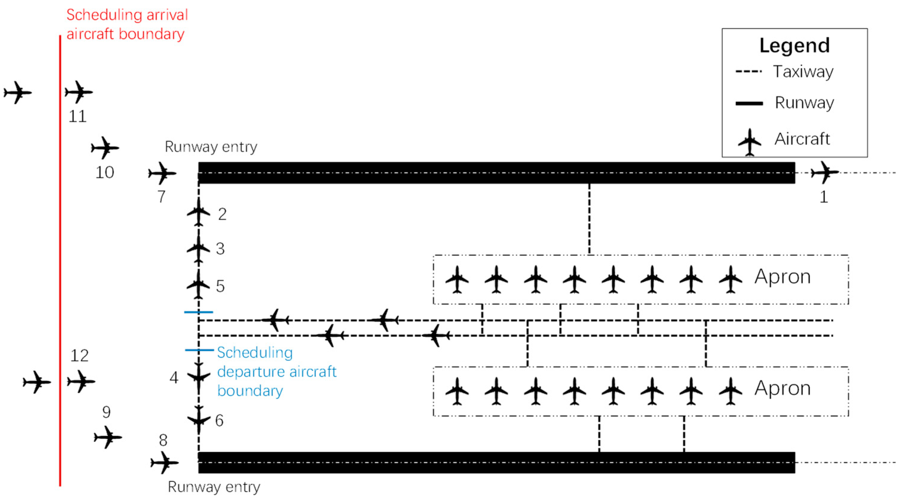
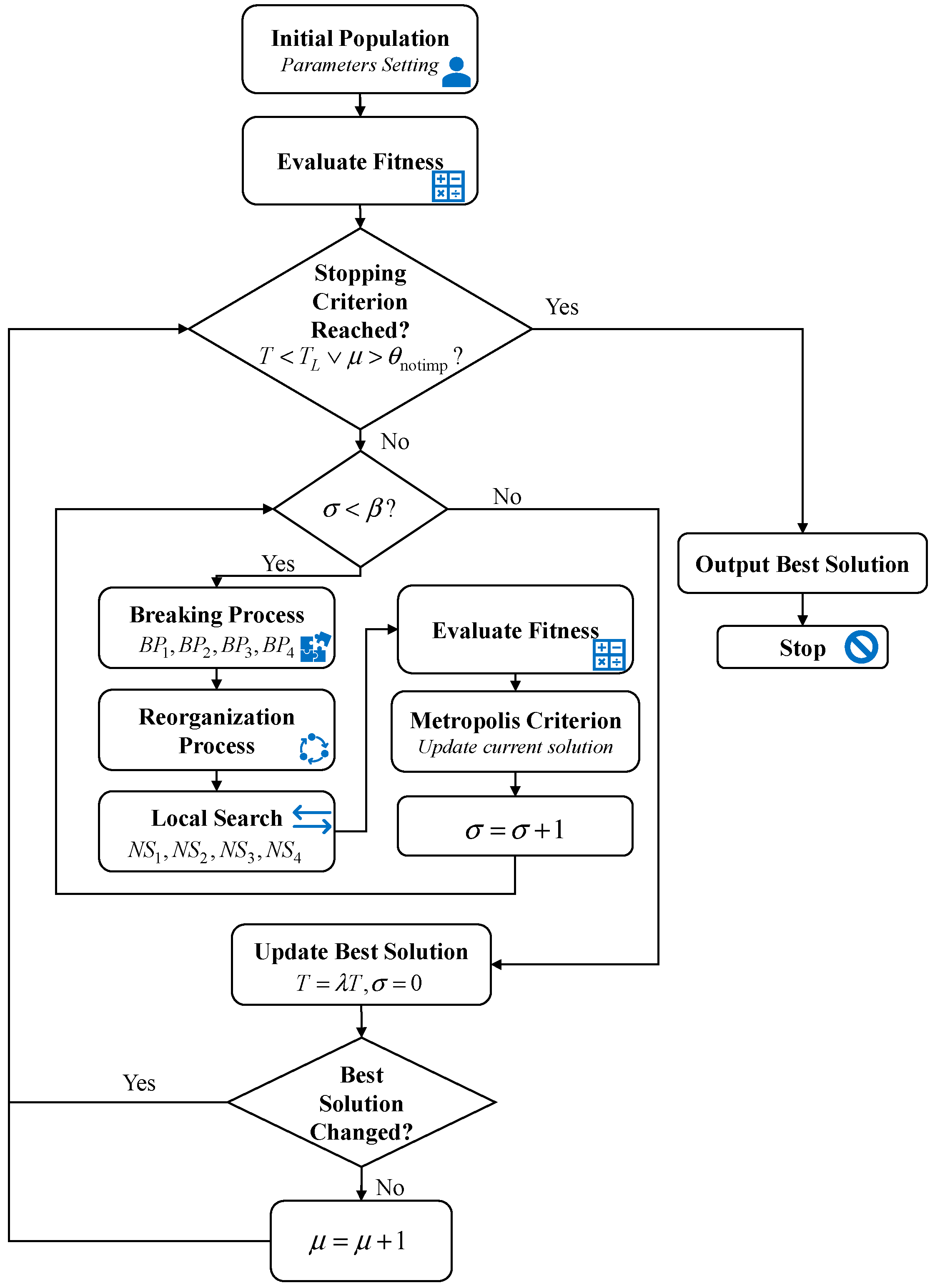
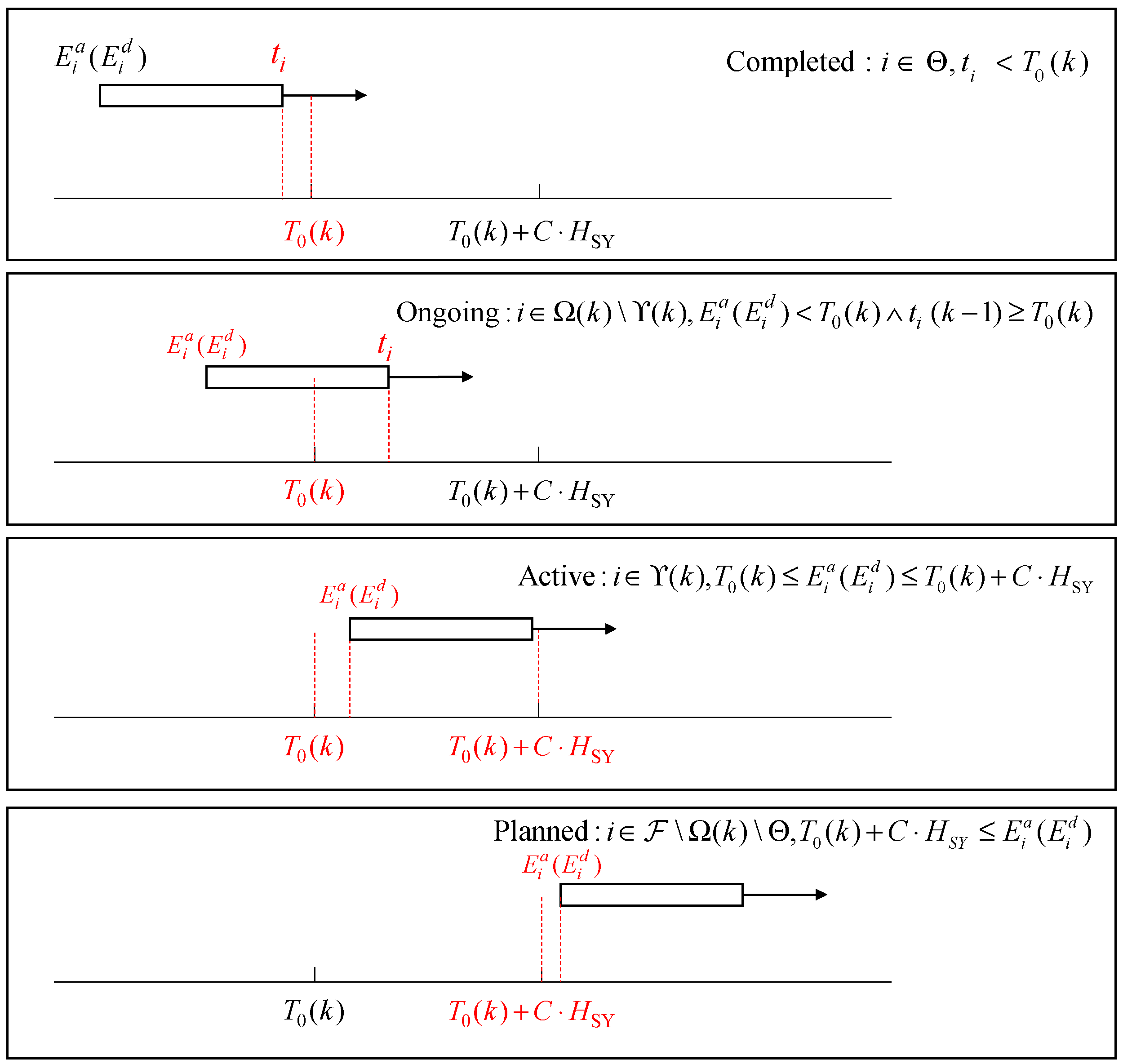
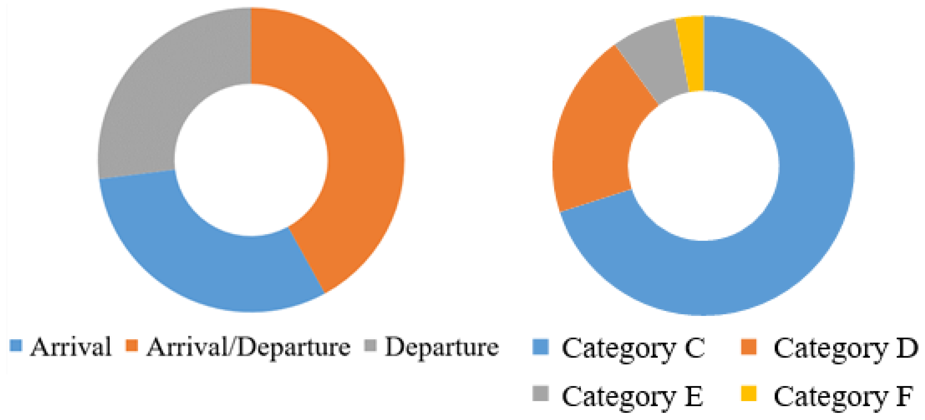
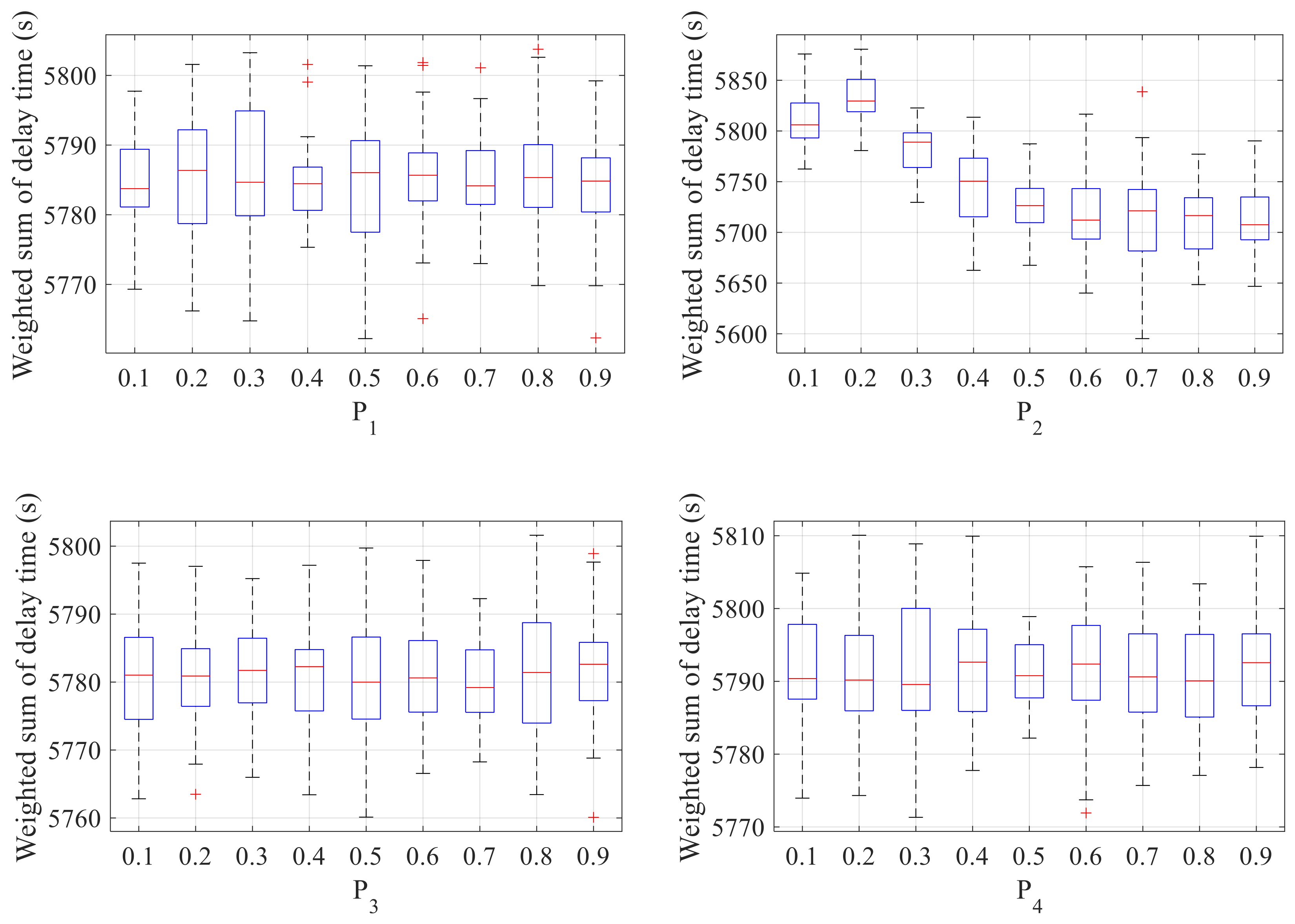
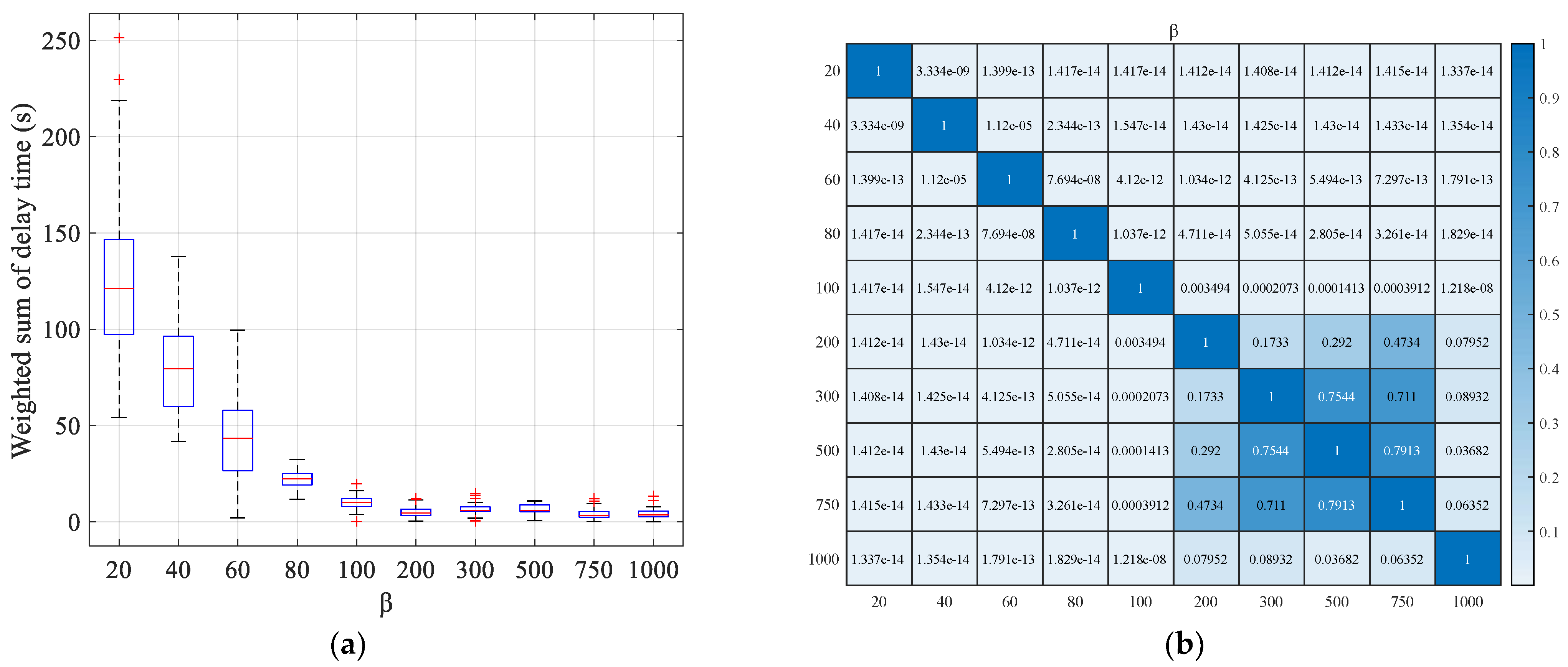
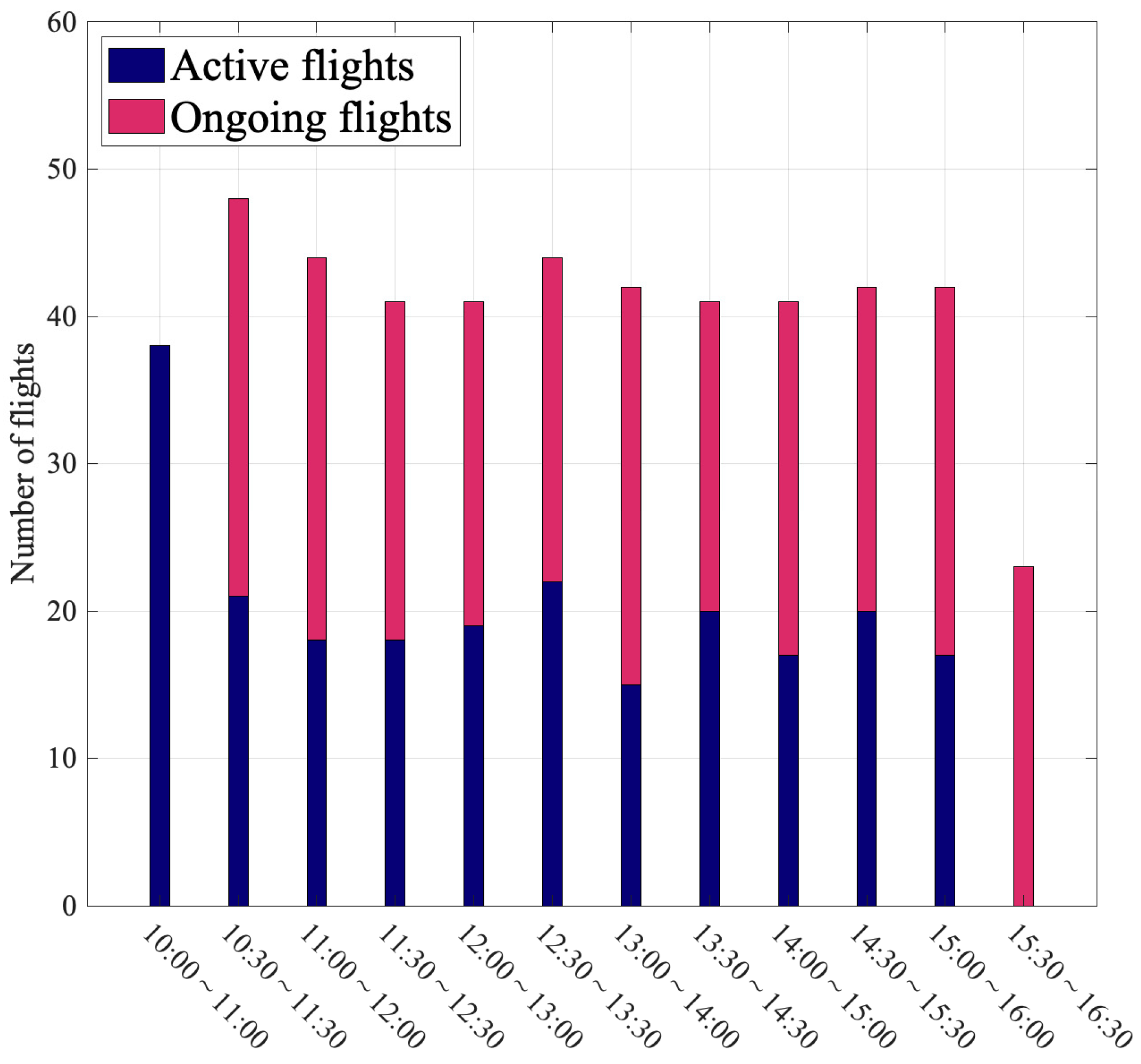
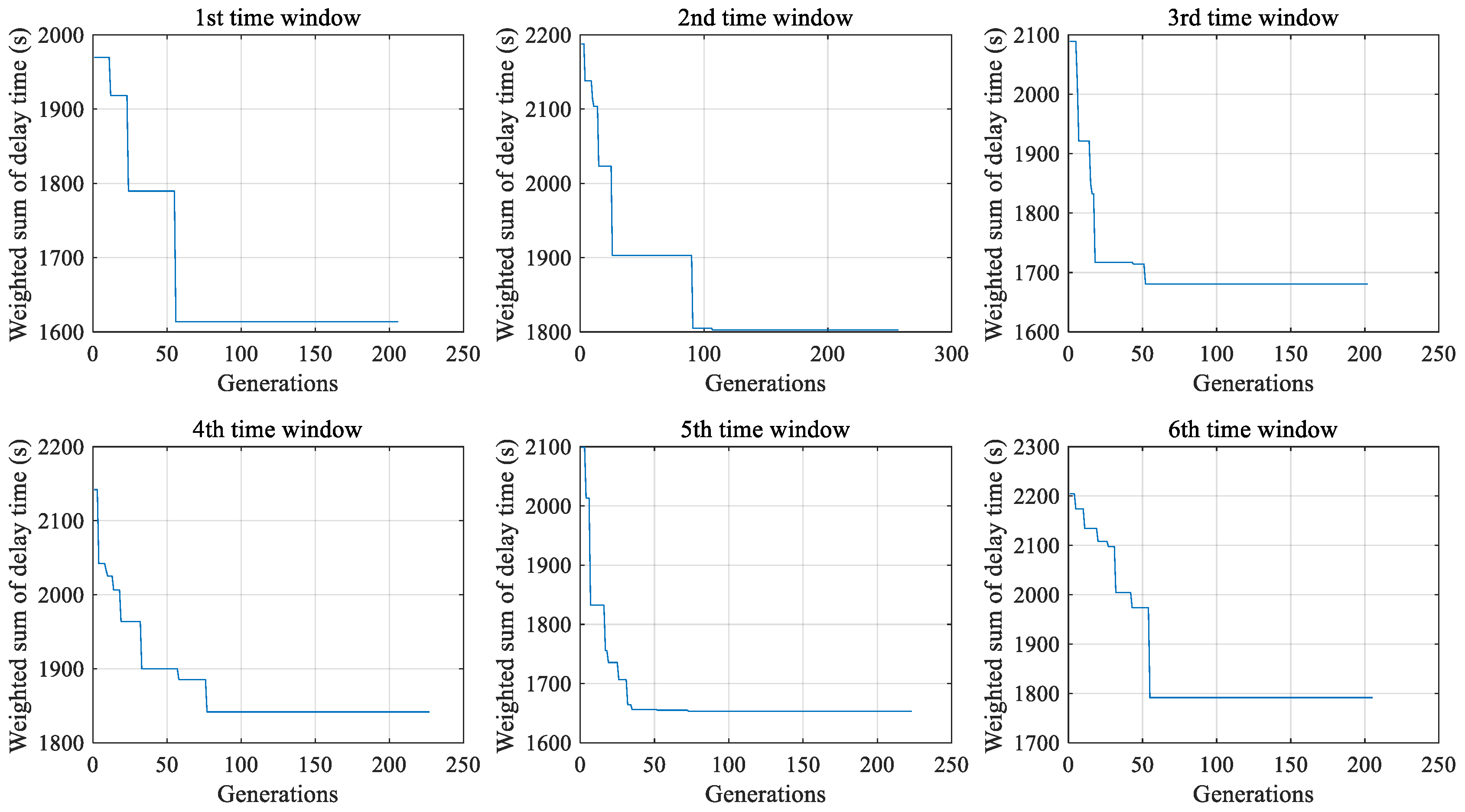
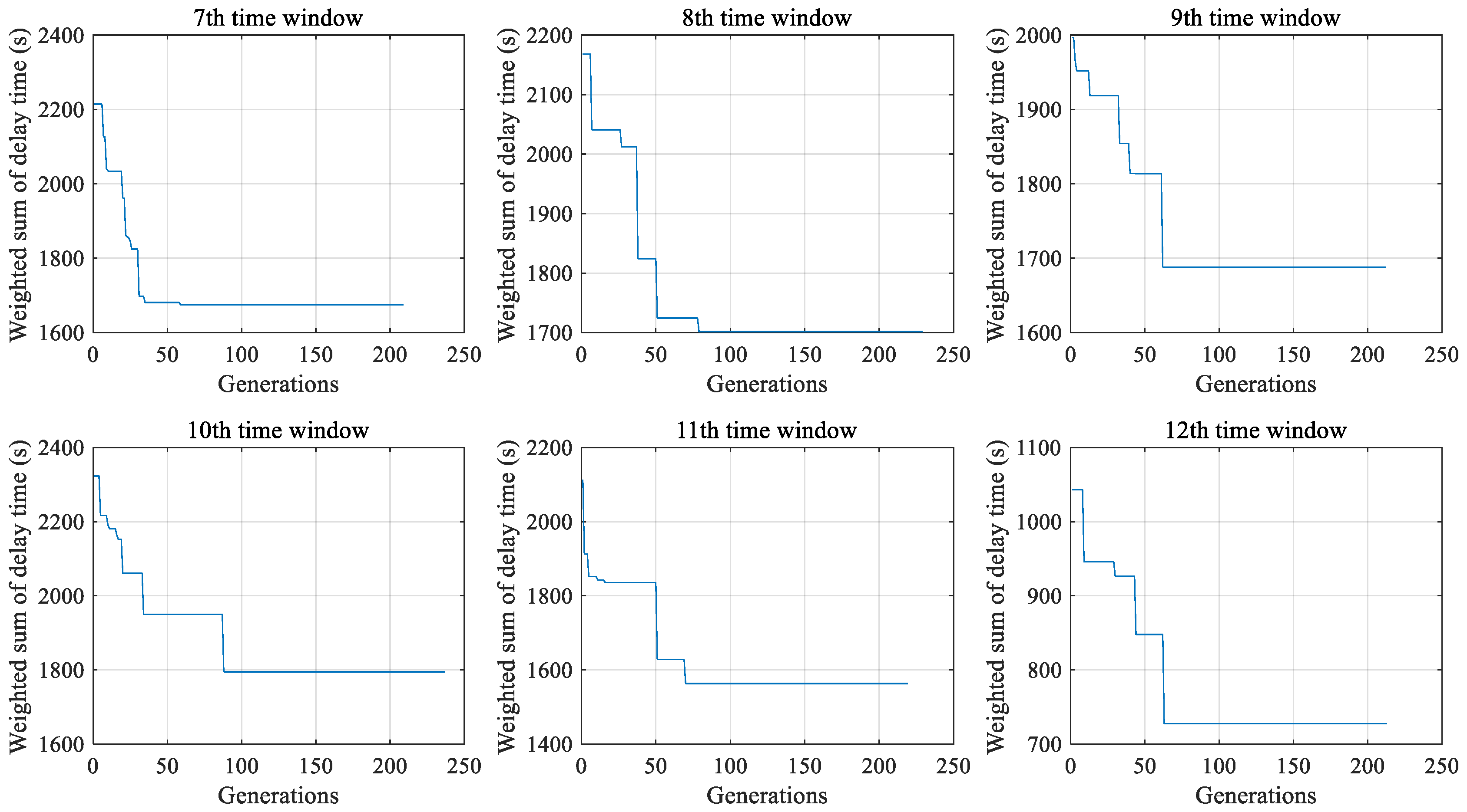
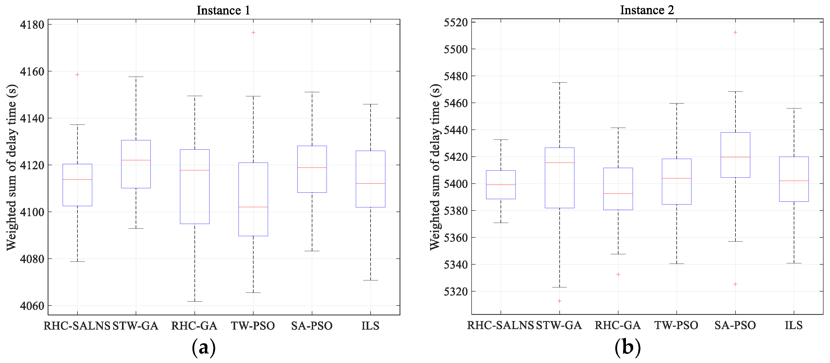
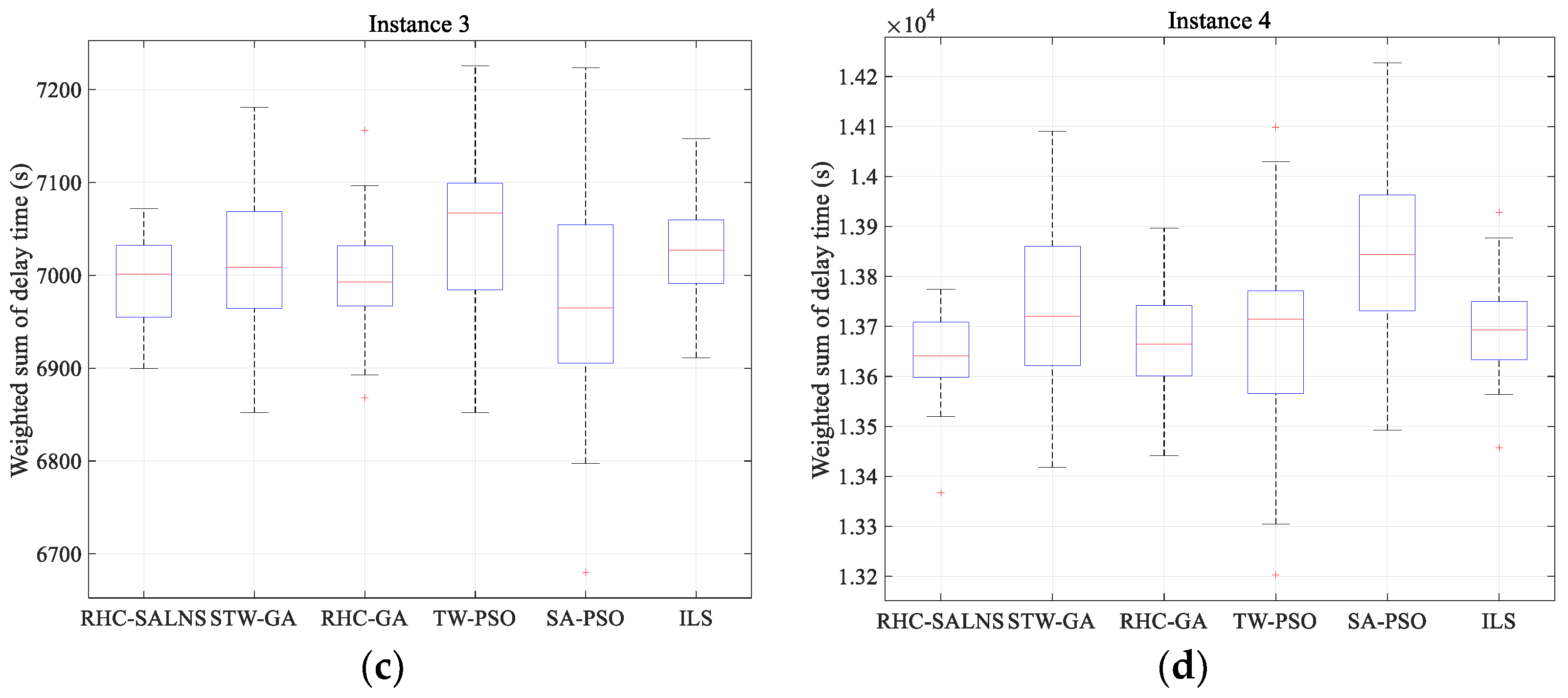
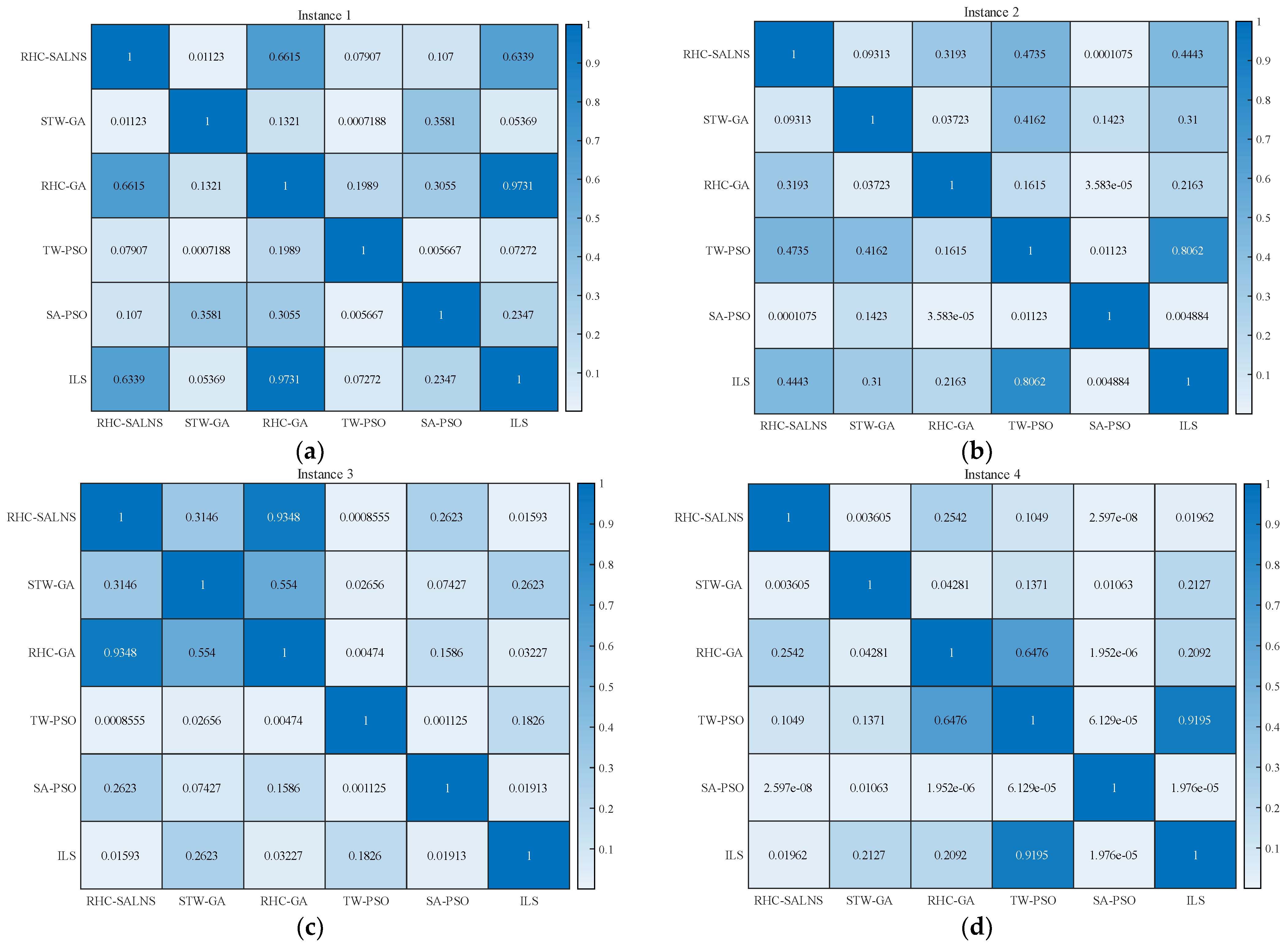
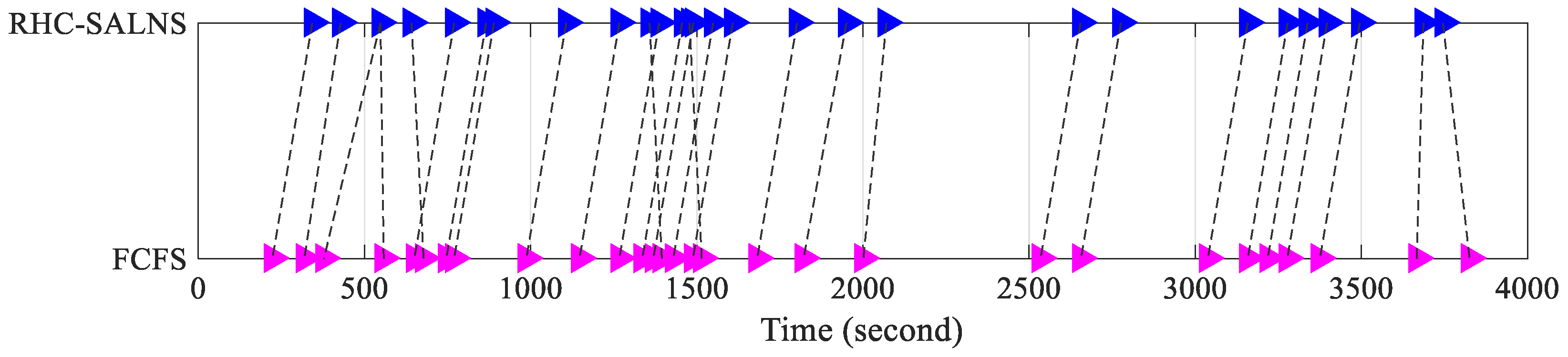
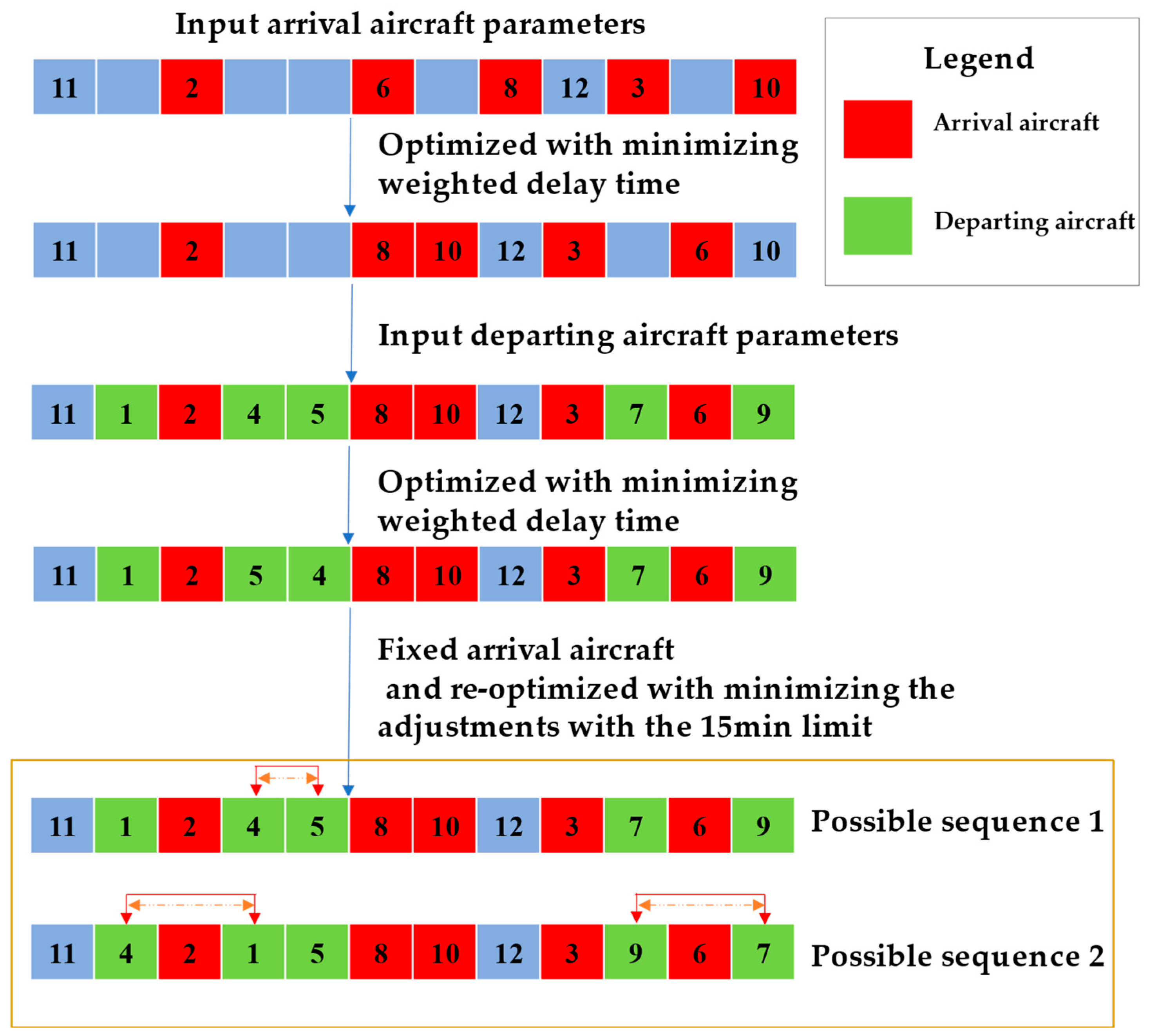
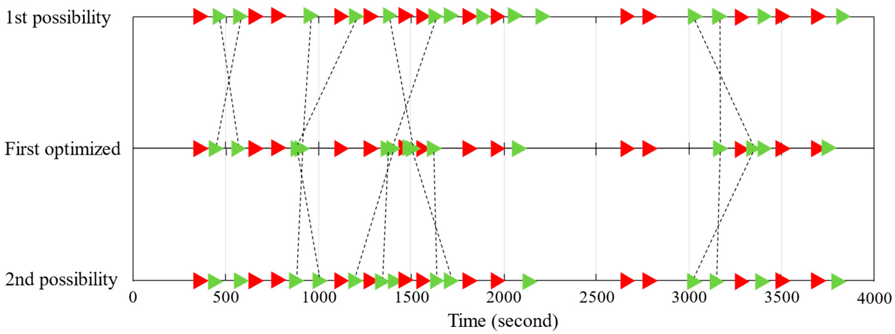
Table 1.
Notations of the ARSP model.
| Sets | |
| The set of aircraft that requiring scheduled during the planning time period | |
| The set of arrival aircraft that land at the airport and stay until planning time period: | |
| The set of departing aircraft that are parked at the airport at the beginning of the planning time period: | |
| The set of arriving-departing aircraft: , | |
| The set of runways available for aircraft, where , | |
| Parameters | |
| The estimated landing time of aircraft: , | |
| The estimated takeoff time of aircraft: , | |
| The minimum runway usage separation time between aircraft: , | |
| Maximum acceptable delay time of arrival aircraft : | |
| Maximum acceptable delay time of departing aircraft : | |
| Runway occupancy time of aircraft : | |
| 1 if departing aircraft and arrival aircraft are a pair of connected aircraft, 0 otherwise: | |
| The minimum connection time between the takeoff time of departing aircraft and landing time of arrival aircraft: , | |
| Extremely large values, applied to simplify the model | |
| Variables | |
| The allocated runway usage time of aircraft: , | |
| is 1 if the aircraft uses the runway , 0 otherwise: | |
| is 1 if aircraft uses the runway before aircraft , 0 otherwise: |
Table 2.
Three-dimensional priority considering three characteristic parameters.
| J | Arrival (Departing) at Peaks (1) | Otherwise (2) | ||||||||
|---|---|---|---|---|---|---|---|---|---|---|
| R | Super (1) | Heavy (2) | Medium (3) | Light (4) | Super (1) | Heavy (2) | Medium (3) | Light (4) | ||
| O | ||||||||||
| Consecutive (1) | 1 | 2 | 5 | 11 | 3 | 6 | 12 | 22 | ||
| Inconsecutive (2) | 7 | 11.5 | 19 | 30.5 | 12.5 | 20 | 31.5 | 48 | ||
Table 3.
The ARSP benchmark instances.
| Instance Name | Number of Aircraft | Time Duration (Second) |
|---|---|---|
| Instance 1 | 150 | 13,200 |
| Instance 2 | 200 | 21,600 |
| Instance 3 | 250 | 25,200 |
| Instance 4 | 500 | 46,800 |
Table 4.
Parameter settings of SALNS.
| Algorithm Framework | Parameters | Value |
|---|---|---|
| LNS | ||
| 0.2 | ||
| 0.6 | ||
| 0.3 | ||
| 0.4 | ||
| SA | ||
| 200 | ||
| 10,000 | ||
| 0.1 | ||
| 0.96 | ||
| 150 |
Table 5.
Optimization results comparison including the computational time for different parameters (, ) setting and the associated final objective values.
Table 5.
Optimization results comparison including the computational time for different parameters (, ) setting and the associated final objective values.
| Instance | Algorithm | Parameter Setting | Total Execution Time(s) | Objective Value(s) | Execution Time per Aircraft(s) |
|---|---|---|---|---|---|
| Instance 2 | SALNS | - | 2110 | 6270 | 10.55 |
| RHC-SALNS | , | 253.0 | 5345 | 1.27 | |
| RHC-SALNS | , | 204.35 | 5638 | 1.02 | |
| RHC-SALNS | , | 492.72 | 5494 | 2.46 | |
| RHC-SALNS | , | 364.8 | 5512 | 1.82 | |
| Instance 3 | SALNS | - | 2938 | 7756 | 10.95 |
| RHC-SALNS | , | 300.12 | 6971 | 1.20 | |
| RHC-SALNS | , | 243.6 | 6774 | 0.97 | |
| RHC-SALNS | , | 567.39 | 7018 | 2.27 | |
| RHC-SALNS | , | 398.2 | 7084 | 1.59 | |
| Instance 4 | SALNS | - | 4557 | 15,164 | 11.54 |
| RHC-SALNS | , | 571.4 | 13,691 | 1.14 | |
| RHC-SALNS | , | 411.21 | 13,664 | 0.82 | |
| RHC-SALNS | , | 1072.53 | 13,535 | 2.15 | |
| RHC-SALNS | , | 742.75 | 14,565 | 1.49 |
Table 6.
Optimization results comparison including the computational time for , and the associated final objective values.
Table 6.
Optimization results comparison including the computational time for , and the associated final objective values.
| Parameter Setting | Time Horizon | Active Aircraft | Ongoing Aircraft | Total Aircraft | Execution Time(s) | Objective Value(s) |
|---|---|---|---|---|---|---|
| 10:00–11:00 | 38 | 0 | 38 | 22.25 | 1565 | |
| 10:30–11:30 | 21 | 27 | 48 | 28.22 | 1667 | |
| 11:00–12:00 | 18 | 26 | 44 | 18.83 | 1826 | |
| 11:30–12:30 | 18 | 23 | 41 | 22.97 | 1543 | |
| 12:00–13:00 | 19 | 22 | 41 | 18.25 | 1763 | |
| 12:30–13:30 | 22 | 22 | 44 | 24.56 | 1745 | |
| 13:00–14:00 | 15 | 27 | 42 | 20.08 | 1821 | |
| 13:30–14:30 | 20 | 21 | 41 | 26.84 | 1649 | |
| 14:00–15:00 | 17 | 24 | 41 | 20.79 | 1923 | |
| 14:30–15:30 | 20 | 22 | 42 | 20.17 | 1687 | |
| 15:00–16:00 | 17 | 25 | 42 | 21.51 | 1785 | |
| 15:30–16:30 | 0 | 23 | 23 | 8.54 | 759 |
Table 7.
The computational results of RHC-SALNS compared to the state of the arts.
| Instance | Algorithm | Average(s) | STD | Execution Time per Aircraft (s) |
|---|---|---|---|---|
| Instance 1 | RHC-SALNS | 4112.3 | 15.8 | 1.21 |
| STW-GA | 4121.1 | 13.8 | 1.18 | |
| RHC-GA | 4111.5 | 23.3 | 1.37 | |
| TW-PSO | 4106.6 | 24.8 | 1.43 | |
| SA-PSO | 4117.7 | 13.9 | 1.20 | |
| ILS | 4113.2 | 17.2 | 1.37 | |
| Instance 2 | RHC-SALNS | 5399.4 | 14.8 | 1.27 |
| STW-GA | 5405.8 | 36.9 | 2.07 | |
| RHC-GA | 5394.2 | 23.3 | 1.34 | |
| TW-PSO | 5402.9 | 28.8 | 1.26 | |
| SA-PSO | 5419.2 | 31.4 | 1.45 | |
| ILS | 5400.7 | 28.6 | 2.12 | |
| Instance 3 | RHC-SALNS | 6995.0 | 46.1 | 1.20 |
| STW-GA | 7011.9 | 68.8 | 3.81 | |
| RHC-GA | 6999.8 | 57.2 | 2.30 | |
| TW-PSO | 7049.2 | 78.7 | 3.24 | |
| SA-PSO | 6978.1 | 114.9 | 2.49 | |
| ILS | 7024.6 | 55.2 | 3.05 | |
| Instance 4 | RHC-SALNS | 13640.7 | 76.8 | 1.14 |
| STW-GA | 13747.2 | 162.0 | 4.23 | |
| RHC-GA | 13665.1 | 95.6 | 2.54 | |
| TW-PSO | 13667.4 | 185.7 | 3.70 | |
| SA-PSO | 13850.8 | 180.1 | 2.81 | |
| ILS | 13693.3 | 89.2 | 3.12 |
Table 8.
The average delay time for departing aircraft and STD under different settings.
| Average Departing Delay Time(s) | STD | |
|---|---|---|
| 5 min | 122.8 | 68.15 |
| 10 min | 126.8 | 134.51 |
| 15 min | 114.14 | 180.17 |
| 20 min | 109.7 | 159.35 |
| 30 min | 108.6 | 139.16 |
| 45 min | 104.58 | 174.72 |
| 60 min | 107.46 | 137.82 |
Table 9.
The result average delay time of 100 Monte Carlo experiments for Instance 2.
| Instance | Execution Time per Aircraft(s) | Average Objective Value |
|---|---|---|
| Instance 2 | 1.47 s | 5582.3 |
Disclaimer/Publisher’s Note: The statements, opinions and data contained in all publications are solely those of the individual author(s) and contributor(s) and not of MDPI and/or the editor(s). MDPI and/or the editor(s) disclaim responsibility for any injury to people or property resulting from any ideas, methods, instructions or products referred to in the content. |
© 2023 by the authors. Licensee MDPI, Basel, Switzerland. This article is an open access article distributed under the terms and conditions of the Creative Commons Attribution (CC BY) license (https://creativecommons.org/licenses/by/4.0/).
Share and Cite
MDPI and ACS Style
Su, J.; Hu, M.; Liu, Y.; Yin, J. A Large Neighborhood Search Algorithm with Simulated Annealing and Time Decomposition Strategy for the Aircraft Runway Scheduling Problem. Aerospace 2023, 10, 177. https://doi.org/10.3390/aerospace10020177
AMA Style
Su J, Hu M, Liu Y, Yin J. A Large Neighborhood Search Algorithm with Simulated Annealing and Time Decomposition Strategy for the Aircraft Runway Scheduling Problem. Aerospace. 2023; 10(2):177. https://doi.org/10.3390/aerospace10020177
Chicago/Turabian StyleSu, Jiaming, Minghua Hu, Yingli Liu, and Jianan Yin. 2023. "A Large Neighborhood Search Algorithm with Simulated Annealing and Time Decomposition Strategy for the Aircraft Runway Scheduling Problem" Aerospace 10, no. 2: 177. https://doi.org/10.3390/aerospace10020177
Note that from the first issue of 2016, this journal uses article numbers instead of page numbers. See further details here.