A Distributed Satellite System for Multibaseline AT-InSAR: Constellation of Formations for Maritime Domain Awareness Using Autonomous Orbit Control

Abstract

Space-based Earth Observation (EO) systems have undergone a continuous evolution in the twenty-first century. With the help of space-based Maritime Domain Awareness (MDA), specially Automatic Identification Systems (AIS), their applicability across the world’s waterways, among others, has grown substantially. This research work explores the potential applicability of Synthetic Aperture Radar (SAR) and Distributed Satellite Systems (DSS) for the MDA operation. A robust multi-baseline Along-Track Interferometric Synthetic Aperture Radar (AT-InSAR) Formation Flying concept is proposed to combine several along-track baseline observations effectively for single-pass interferometry. Simulation results are presented to support the feasibility of implementing this acquisition mode with autonomous orbit control, using low-thrust actuation suitable for electric propulsion. To improve repeatability, a constellation of this formation concept is also proposed to combine the benefits of the DSS. An MDA application is considered as a hypothetical mission to be solved by this combined approach.

1. Introduction

Strong and robust maritime security arrangements are required to contribute to the Intelligence, Surveillance, and Reconnaissance (ISR) operations and Maritime Domain Awareness (MDA), which can be accomplished using satellite technologies. This approach based on space information becomes essential for countries in the southern hemisphere, with a sizeable maritime domain to protect in terms of sovereignty and sovereign rights, naval assets, infrastructure, resources, and people [1,2,3]. These capabilities can significantly help with resource and biodiversity preservation, economic and environmental sustainability, disaster mitigation, and security at marine, in addition to supporting safety and security at sea [4]. This is especially true for isolated regions such as Australasia [5,6] and resource-rich regions such as the Gulf of Guinea [7], the South China Sea [8], Micronesia [9], the Argentine Sea [10], the Mediterranean Sea [11] and the Indian Ocean [12], just to name but a few. According to the United Nations (UN), Illegal, Unreported and Unregulated (IUU) fishing is a major factor contributing to more than 90% of global fisheries stocks getting fully exploited, overexploited, or depleted, affecting regions most impacted by climate change. This practice also accounts for one-fifth of global fisheries catches, which can be worth up to USD 23.5 billion per year, making it the third most lucrative business natural resource crime after timber and mining [13]. For MDA, satellites can provide the data for tracking ship movements, i.e., for ISR operations and data for observing the marine environment, such as meteorological and oceanographic conditions. In 2014, the International Maritime Bureau (IMB) estimated that maritime piracy caused USD 16 billion in economic losses annually, mostly as a result of theft, transportation delays, insurance costs, anti-piracy measures, etc.

The Distributed Satellite Systems (DSS) involves a set of small satellites working together which can simultaneously cover larger areas and outperform a single large (i.e., monolithic) satellite, which is often more expensive and less effective. DSS has many advantages, including easier design, faster build time, lower replacement costs and increased redundancy [14,15,16,17]. One issue is to keep the formation geometry (required to accomplish the mission) while avoiding inadvertent collisions due to uncertainty in the state of the formation and/or failures. Recent research focuses on various control strategies to address these changes, including the possible adoption of artificial intelligence (AI) techniques [18,19]. 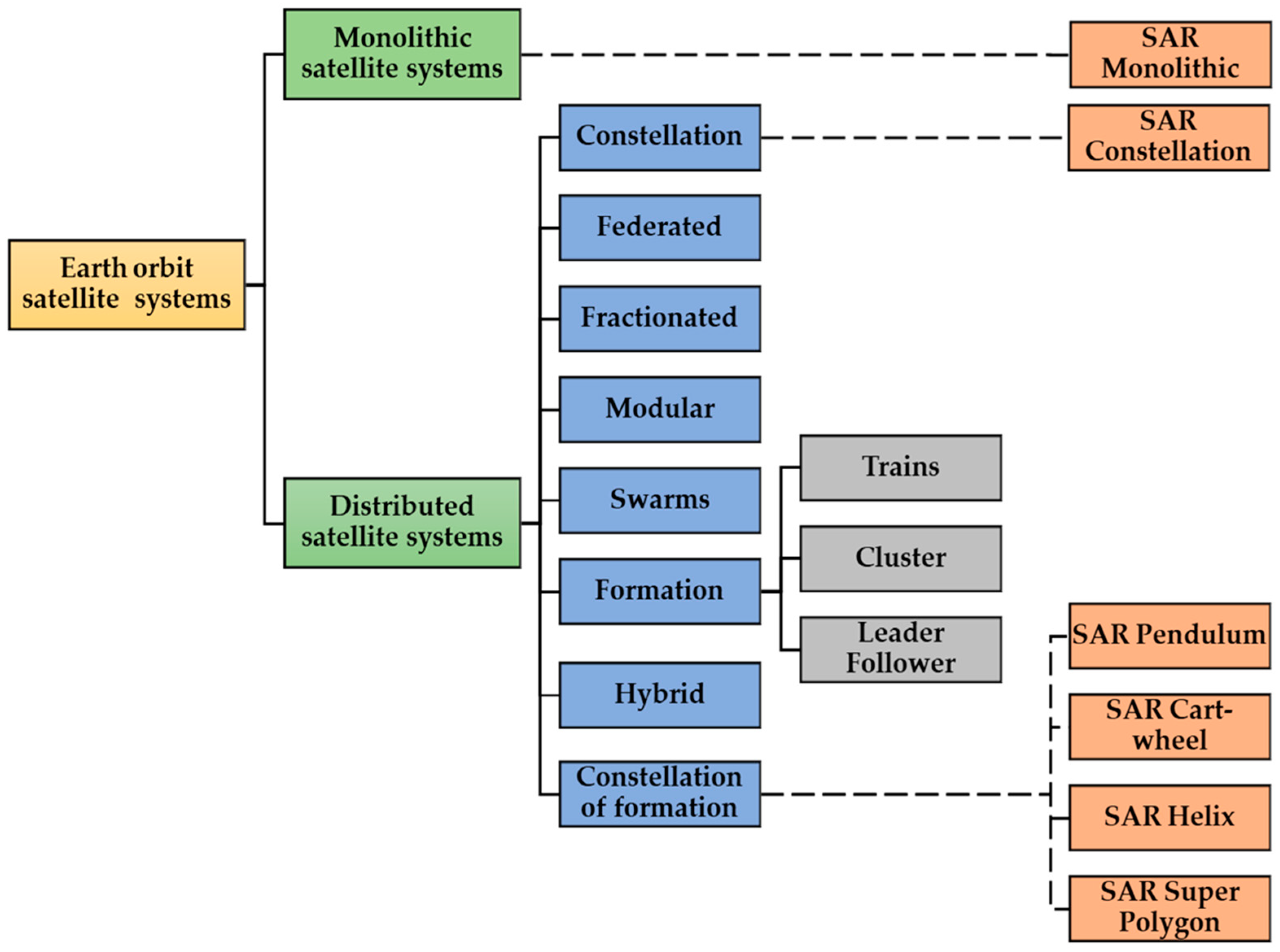Figure 1 depicts a possible classification and example of Synthetic Aperture Radar (SAR) satellite mission types [20,21]. The satellite systems are classified into monolithic and distributed satellite systems, and the latter is divided into several possible implementation branches as the constellation (flying far from each other, without relative navigation/control), Formation Flying (close flight, requires relative control) and other options as swarms or hybrid approaches [18].

The implementation of a control law requires communication between the satellites in each formation, i.e., Inter Satellite Links (ISL), in such a way that all the absolute positions are known at least by one of the satellites, while all of the satellites receive all the relative errors and the center of mass acceleration command in order to implement the associated force. ISL allows for satellite-to-satellite communication on each DSS formation and there are many possible implementations, as shown by Liz Martinez et al. [22]. A direct solution is given by the Star topology, where the follower satellites of the formation communicate this navigation state to the chief, and hence the chief can broadcast this information to all the followers, also including its own navigation state and the relative navigation with respect to each of the followers. Figure 2 shows this and other feasible topologies, with the full-duplex ISL being represented by double arrows. By including reactive components into the architecture, ISL allows the DSS operations to be enhanced and data to be processed on-board the satellite for timely operation, which makes intelligent DSS (iDSS). The ground station network and/or geostationary satellite service can be used to facilitate communications between satellites of different formations, which may be useful to perform constellation reconfigurations and process collision avoidance alarms from external objects [16]. As the communications become part of the control loop, a complete infrastructure to validate autonomous orbit control shall be able to emulate the inter-satellite links, as proposed in [23]. ISL is an essential component of the DSS astrionics architecture. They make it possible for rapid data sharing between satellites and AI-based on-board data processing [24,25,26], which relieves some of the tasks that were previously carried out by the ground segment. In this way, the information generated within each formation can be combined on-board (for instance, processed on one satellite and distributed within each formation using a Star ISL, as shown in the following figure) and delivered directly to the user, which is crucial on a surveillance application as MDA. We propose a single pass and on-board generation of the interferogram created by the combination of the SAR acquisitions of all the satellites of each formation, which will allow to obtain a timely high-quality product. This improves both the efficiency of the downlink and the operational effectiveness of the system, as measured by a decreased amount of work for human operators and more streamlined mission management.

In this research work, a constellation of formations is proposed to combine the benefits of the repeat cycle given by the constellation with the single-pass products allowed only by the Formation Flying distribution. An example of a monolithic SAR satellite was the Envisat [27], which provided a repeat cycle of 35 days. To perform interferometry, the product constructs the interferogram from different acquisitions of the same scene, which in this case is separated for 35 days. The constellation solution reduces the revisit time to a few days as the Satellite System for Emergency Management (SIASGE) system (Satélite Argentino de Observación COn Microondas (SAOCOM-1) and Cosmo-Skymed SAR constellations). However, this could not be enough for applications needing real-time generation of the interferogram.

In this study, a real-time interferometry is required for the MDA application, which needs to be computed on every single pass over a given target zone or area of interest (AOI). This requirement may be derived from two main motivations: the need for a fast determination of the interferogram, and the need for high coherence in the interferometry, in order to avoid artifacts caused by differences in the background of the scene due to the atmospheric changes or other effects not related to this specific application. Furthermore, as a new DSS architecture type, a constellation of these formations is considered to keep this feature and reduce the revisit time. This work also investigates the possibility of allocating control accelerations among satellites on each formation as a function of the formation objective (relative geometry) and the constellation objective (ground track repetition cycle period). The following contributions were made:

• A safe multi-baseline shifted-Helix Formation Flying is proposed for Along-Track Interferometric Synthetic Aperture Radar (AT-InSAR) Distributed Satellite System (DSS), in the context of a Maritime Domain Awareness (MDA) mission over Australia.
• Autonomous orbital control is evaluated for reconfiguration and maintenance of this DSS formation.
• For an increased revisit of maritime surveillance, a novel DSS Archetype, “Constellation of Formations”, is proposed, with an associated autonomous control law evaluated by simulations.

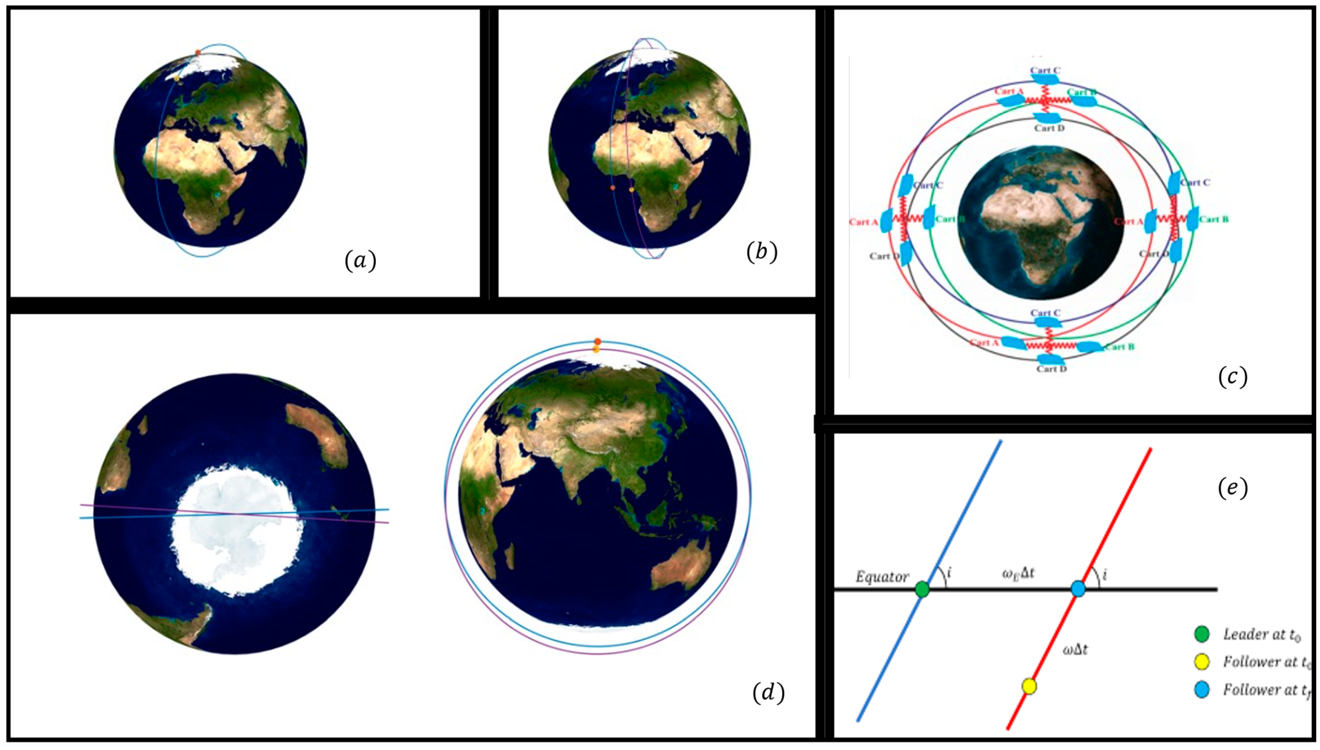
The objective of this work is not to define the constellation parameters but to propose a concept for its implementation adding autonomy by means of this two-level (constellation/formation) autonomous orbit control. Single pass interferometry is selected to maximize the coherence, which can be achieved by satellites flying very closely using a Formation Flying (FF) approach, as was implemented on TanDEM-X [28]. This pioneering mission generated new SAR products by defining the acquisition modes as a function of the relative orbits between both satellites, each of them having a complete SAR instrument. Examples of these relative orbits are given in Figure 3. Satellite Formation Flying (SFF) is the coordination of multiple neighboring satellites to accomplish an objective/goal stated in terms of the relative orbits between them. There are various configurations of Formation Flying missions in order to satisfy the user requirements. Each configuration can be obtained by small changes in the orbital parameters of each deputy satellite with respect to the nominal parameters of the chief satellite. In order to meet the needs of the users, different configurations of Formation Flying missions have been proposed. SFF can be classified depending on the configuration, mode of operation, and other factors.

2. Synthetic Aperture Radar

A satellite radar instrument produces and transmits its own energy using a known microwave signal pattern, then records the reception of that signal reflected back after interacting with the earth’s surface. When this instrument moves with a known velocity relative to the earth’s surface, the reflection also adds azimuthal information due to the Doppler frequency deviation and is referred to as SAR data collection. SAR data must be interpreted differently from optical images because the signal responds to surface characteristics such as structure and wetness rather than being a static image. Compared to optical technology, SAR technologies can “see” through the darkness and can operate at any time of the day. Moreover, for longer microwave bands such as the L-band, the SAR instrument can also see through clouds, fog, and rain. This robust operation allows for tracking the trends in habitat, water, and moisture levels, the consequences of natural or human disturbance and variations in the earth’s surface as a result of quakes or sinkhole openings. These products are created by analyzing the reflections of signals off a target location and measuring the two-way transit time back to the satellite, its frequency deviation, and the polarization changes. The SAR interferometry technique “interferes” (differences) with two SAR images of the same area, producing maps called interferograms that reveal ground-surface displacement (range change) here between the two time periods. The phase differences are used to extract information about the captured objects (in comparison to a single image). As a result, at least one aspect (“Baseline”) must differ between the images.

Future SAR missions will benefit from increased capability, reliability, and flexibility as a result of this spatial separation [28]. Applications for multistatic SAR systems include single-pass cross-track and along-track interferometry, spaceborne tomography, wide-swath imaging, resolution augmentation, ground-moving target acquisition, interference suppression, and multistatic SAR imaging. Simultaneous data collection from numerous satellites reduces temporal and atmospheric disruptions, enhances performance, and allows the identification of rapid changes.

AT-InSAR systems are employed to estimate the radial velocity of targets moving on the ground by combining the interferometric phases, which are acquired by combining the two intricate SAR images obtained by two antennas spatially separated along the platform moving direction [29]. The AT-InSAR can be used in various applications such as monitoring real-time traffic management, ocean currents, coastal surveillance, ice drift, etc. In AT-InSAR, the baseline difference is an along-track distance, with a magnitude depending on the mission type, and determines the time difference associated with the pass of the satellite over the particular target, hence measured in seconds for single pass interferometry (two consecutive satellites looking at the same target) or days/years for multiple-pass interferometry (i.e., to process a stack of images taken on different passes over the same scene by the same satellite, other different satellites in a SAR constellation). 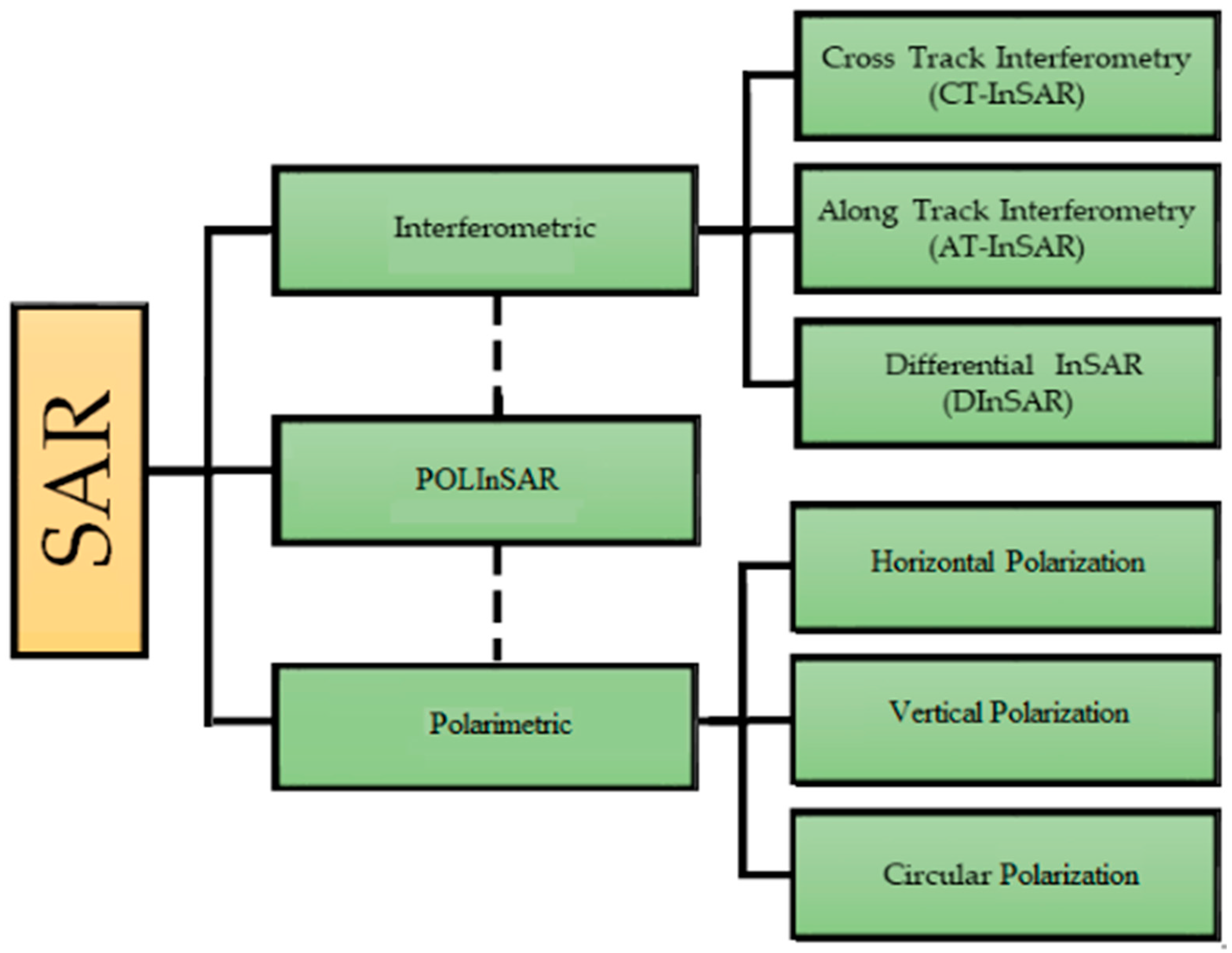Figure 4 shows different types of SAR in a simplified classification. The two main branches, interferometric and polarimetric, can also be combined as in the polarimetric SAR interferometry (POLInSAR) techniques [30].

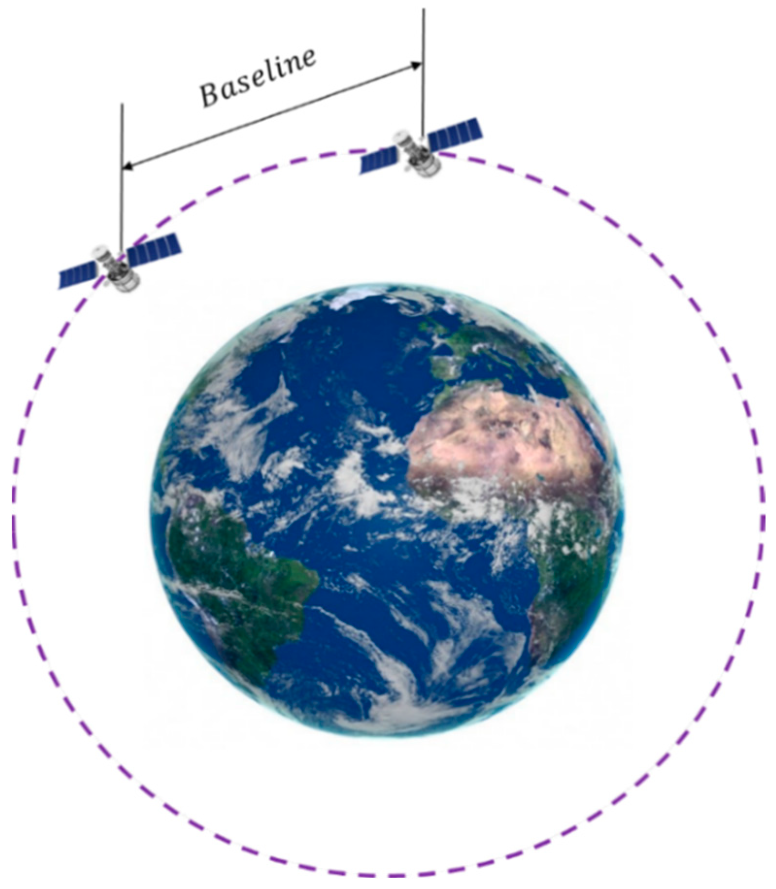
The interferometric SAR missions can be implemented by multi-static SAR, which is characterized by their relative position or equivalent time, known as the baseline. This subfield of SAR categorization will serve as the primary focus of the analysis. Some baseline types usually implemented on SAR interferometric missions are shown in

Table 1. Some baseline types for interferometric SAR [28].

Baseline	SAR Type	Measurement and Application
$\Delta \phi$(look angles difference)	Across-Track	Topography, digital elevation models
$\Delta t = ms,\dots , s$	Along-Track	Ocean currents, moving object detection
$\Delta t = days$	Differential	Glacier/ice fields, lava flows, hydrology
$\Delta t = days, \dots , years$	Differential	Subsidence, seismic events, volcanic activities, crustal displacements
$\Delta t = ms, \dots , years$	Coherent Estimator	Sea-surface decorrelation times, land cover classification

, and the baseline position difference is shown in Figure 5 for Along-Track interferometry. These baselines can be implemented in multiple passes, on which the interferogram is constructed with data of points of view obtained after several days when there is a repetition cycle on the ground track, or along a single pass when the multi-static SAR is composed of neighboring satellites flying in formation. The latter may improve the SAR product in several ways, as the interferogram can be obtained in almost real-time.

In SFF, there are several topologies to implement the relation between the satellites, for instance, the typical leader-follower approach. In this case, a Deputy satellite (also called follower or secondary) can choose from among the several formation geometries described previously to follow the chief, which can be reconfigured on-board [31]. The chief may also have an autonomous control objective to maintain the absolute orbit (for instance, drag-free), which is therefore followed by the Deputy. Beyond the topology, there are objectives to follow the absolute orbit (for example, to guarantee a constellation repeat cycle for a desired coverage) and other objectives to follow a specific relative orbit geometry within the formation. A more general approach will be proposed to deal with these two types of objectives, to be presented as a Constellation of Formations. The type of formation useful for the MDA application is first taken into account, followed by simulation results using low-thrust continuous control for formation maintenance and reconfiguration.

3. Robust Multiscale AT InSAR

As mentioned previously, the Along Track formation relies on precise control of the along-track separation in order to avoid collision between the leader (or chief) and follower. This entails a risk due to the typical drift between satellites in case the orbit control was not active for a period of time. On the other hand, the possible need for two different baseline scales simultaneously multiplies the risk, as there are now three possible collision events if only one more follower satellite were added to the configuration. D’Amico showed in [32] a description of a relative orbit in terms of Relative Orbital Elements $\delta \underset{\_}{\alpha } = \left(\delta a, \delta \lambda , \delta \underset{\_}{e} ,\delta \underset{\_}{i}\right)$, where $\delta \underset{\_}{e}$ = ($\delta e_x, \delta e_y$) is the relative eccentricity vector and $\delta \underset{\_}{i}$ = ($\delta i_x, \delta i_y$) is the relative inclination vector. The orbit phase difference is given by $\delta \lambda$, while the semi-major axes’ relative difference is $\delta a$. A safe formation is guaranteed when $\delta \underset{\_}{e}$ and $\delta \underset{\_}{i}$ are parallel or anti-parallel, for $\delta a=0$. A strict AT-InSAR formation only has an orbit phase difference between satellites, thus it is not possible to guarantee the safe condition (as $\delta \underset{\_}{e}=\delta \underset{\_}{i}=\underset{\_}{0}$, here parallelism cannot be evaluated). Here a variation of this along track formation is proposed and as follows:

• To add a small helix component to each follower relative to the chief, where the across-track component is one order of magnitude smaller than the chief/follower along-track baseline.
• To scale the chief/follower relative eccentricity and relative inclination vectors in order to generate low-risk “pipes” for each satellite.

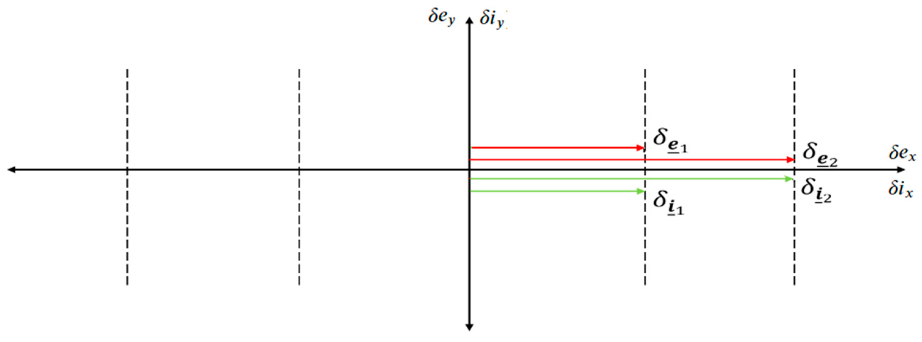
Figure 6 shows a particular case of a parallel relative eccentricity and relative inclination vectors for two followers with respect to the chief.

Notice that the difference between the followers also preserves the relative eccentricity and relative inclinations vectors as collinear, therefore achieving a safe condition. This formation can include more followers by adding other scales on the same axis, preserving the collinearity between the relative eccentricity and inclination vectors for the given follower. On the other hand, different along-track baselines could be chosen for each of these followers. As the chief orbit is sun-synchronous and frozen, the satellite altitude and relative orbit baselines are guaranteed to repeat for the same latitude; hence the interferogram products generated on each pass have geometric coherence between different passes, enabling to perform differential interferometry by taking a set of images generated by the SAR system for the same zone. Moreover, the multiple along-track channels make it possible to track different velocity ranges for the targets on the Earth’s surface, see [29], which can also be compared along the same pass by adding followers with different along-track baselines with the safe configuration previously presented. The following equation, adapted from [32] (Equation (1)), defines a metric $\delta r_{rn}^{min}$ to evaluate the minimum distance, on the radial/normal plane, between two satellites in a formation, by using the Relative Orbital Elements, as follows, for a chief orbit with semi-major axis $\left(a_c\right)$:

$$\delta r_{rn}^{min}=\frac{\sqrt{2}{a}_c \left|\delta \underset{\_}{e}·\delta \underset{\_}{i}\right|}{\sqrt{\delta e^2+\delta i^2+\left|\delta \underset{\_}{e}+\delta \underset{\_}{i}\right|·\left|\delta \underset{\_}{e}-\delta \underset{\_}{i}\right|}}$$

(1)

where $\delta e=\left|\delta \underset{\_}{e}\right|$ and $\delta i=\left|\delta \underset{\_}{i}\right|$. This metric will be used in the following section to evaluate the stationary regime after a reconfiguration using an autonomous orbit control.

4. Autonomous Orbit Control

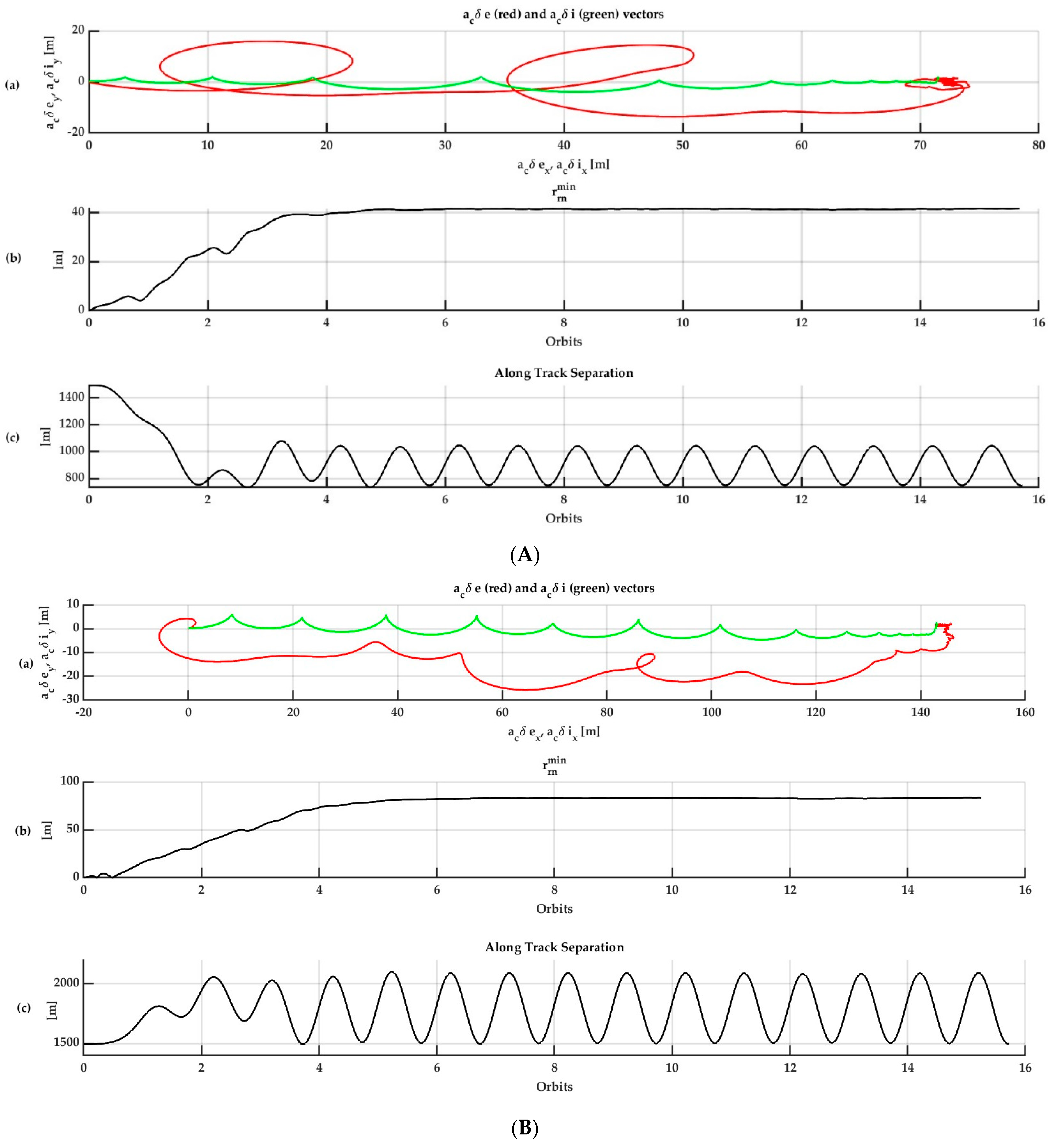
The relative orbital elements are used by an autonomous feedback orbit control law derived in [31]. This control law guarantees a bound control acceleration expressed in the Radial, Transverse, Normal (RTN) frame. Figure 4 shows the simulation results for two followers after a reconfiguration maneuver starting with a pure along track (unsafe) condition. Figure 7a shows the eccentric vector $\delta \underset{\_}{e}$ and the inclination vector $\delta \underset{\_}{i}$ components, which achieves a final state close to the pattern defined in Figure 6. Figure 7b shows the evaluation of the radial/normal minimum distance metric $\delta r_{rn}^{min}$. Figure 7c shows the along-track separation, which can be defined dynamically for each of the followers. As there is a small helix component added to the along-track formation, there will also be an oscillation on the along-track distance, whose amplitude doubles the amplitude of the radial/normal component. The proposed geometry only sketches the idea of the relative geometry, while the definition of the parameters should be given by the application and can be changed dynamically using autonomous orbit control. The reconfiguration between the unsafe along-track formation and the safe one proposed in the previous section is examined in this section.

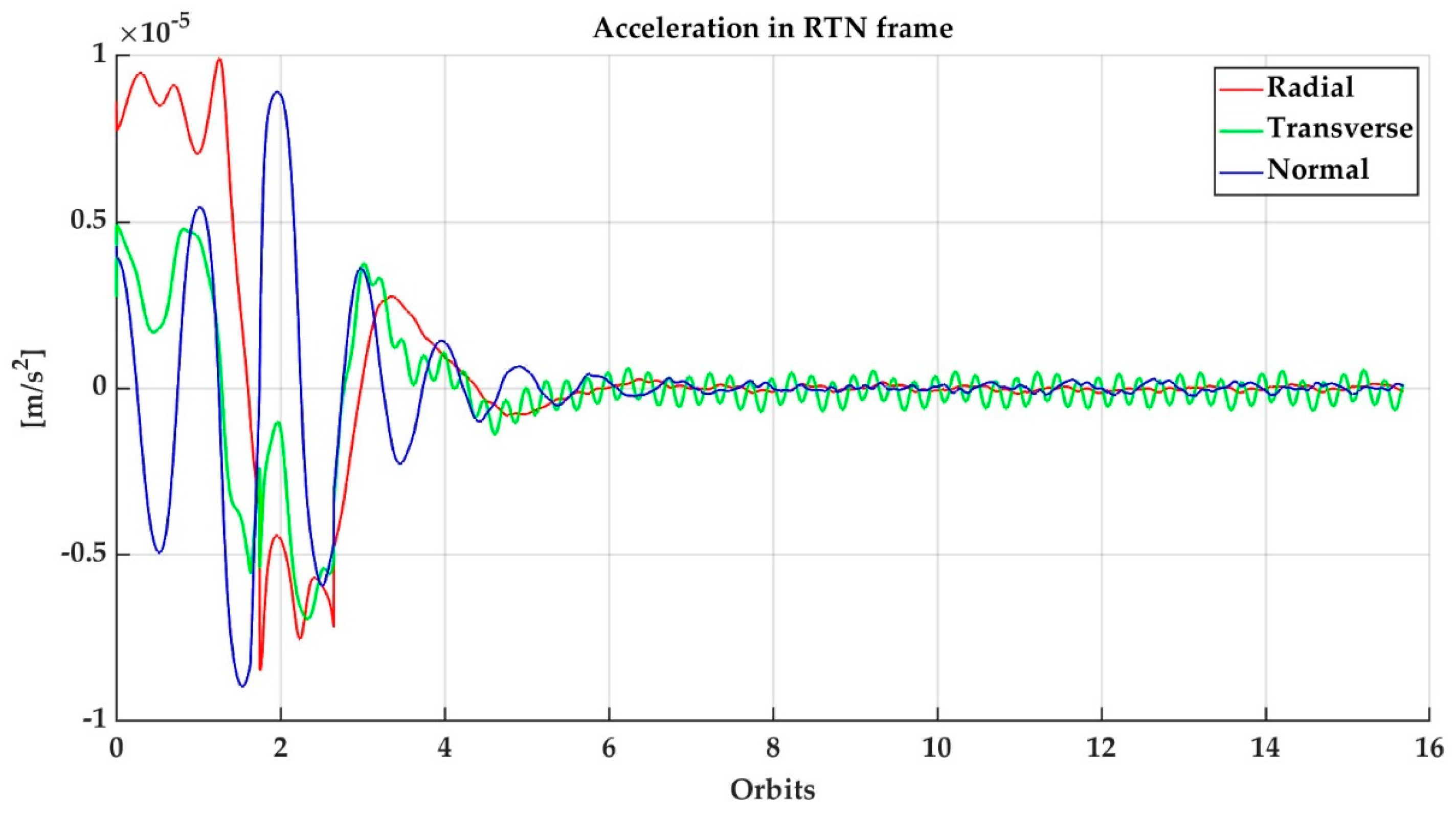
Figure 8 shows the result for follower 1 with an orbit control period of 20 s, and assuming here ideal orbit navigation. For a satellite mass of 100 kg, the simulated thrust bound would be 1 mN in all directions. Figure 9 shows the coordinates given by the difference between relative perigee angle $\phi$ and relative ascending node angle $\theta$, with respect to the norms of the relative eccentricity $\delta \underset{\_}{e}$ and relative inclination $\delta \underset{\_}{i}$ vectors, scaled by the chief’s semi-major axis $a_c$ [32]. Notice that the beginning of the trajectory is at the origin of $\delta e$and $\delta i$, and thus it is not under a safe condition, while at the end, the difference $\varphi -\theta$ is nearly zero (i.e., the relative eccentricity and inclination vectors are collinear) while the stationary relative eccentricity and inclination norms are approximately 40 m when scaled by the semi-major axis. Therefore, the reconfiguration achieves the desired baseline and the required safe condition.

5. Constellation of Formations

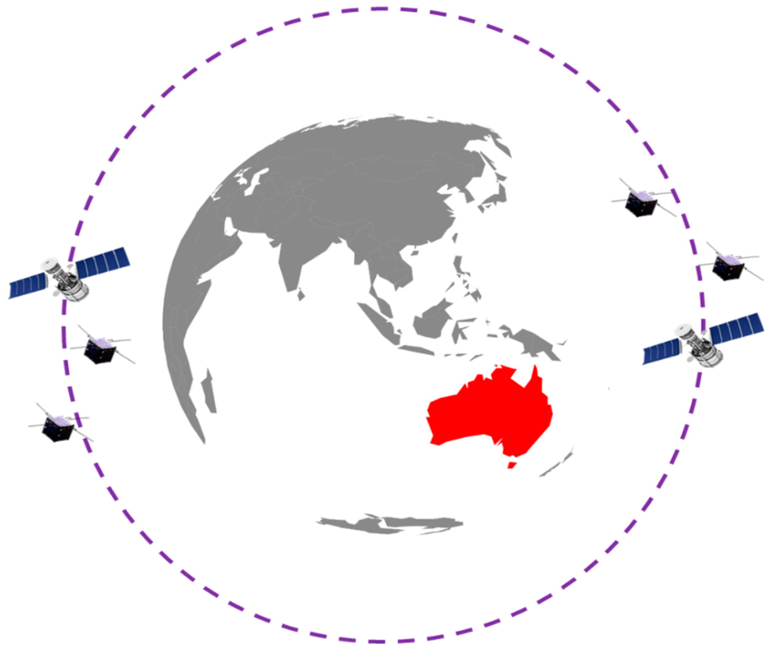
The formation presented in the previous section has a ground-track repeatability described by the repeatability of any of the ground tracks of the satellites in the formation. These ground tracks limit the observation coverage for a given instrument’s field of view. A constellation of satellite formations is proposed to increase the repeatability and coverage of the desired DSS while keeping the formation advantages. Figure 10 shows an example of two formations flying in a constellation. Notice that each formation preserves the single-pass SAR interferometry objective. On the other hand, the resulting constellation can be designed by using the center of mass of each formation as the constellation-equivalent satellite.

Let the constellation $C=\left\{F_1, F_2, \dots , F_{Nc}\right\}$ be a set of $N_c$ formations $F_i$, each of them composed by $N_{F_i}$ satellites, i.e., $F_1=\left\{s_{1,1}, s_{1,2},\dots ,s_1{,}_{N_{F_1}}\right\}$, $F_2=\left\{s_{2,1},s_{2,2},\dots ,s_2{,}_{N_{F_2}}\right\}$, etc. As each satellite $s_i{,}_j$ belongs to the formation $F_i$ and to the constellation C, there are at least two objectives for the orbit controller:

• $O_F$—To keep the relative orbit of the satellite $s_i{,}_j$ within the formation $F_i$.
• $O_C$—To keep the formation $F_i$ in the constellation $C$.

The formation objective $O_F$ has been treated in the previous section by using the relative orbital elements to describe the feedback error. However, there is flexibility in the implementation of the control law that designers can now use, as for any given acceleration control determined by the follower relative orbit feedback law, designers can implement it on the follower alone, on the chief satellite alone, or on both. In this case, the freedom is used to implement the formation orbit control laws in such a way that it does not modify the dynamics of the formation’s center of mass.

The constellation objective $O_C$ is stated considering the absolute orbit elements as generated by the constellation design, which is typically free of non-conservative forces, i.e., without drag and solar pressure effects, and with a certain reduced order model of the gravitational effects. On the other hand, to build the constellation control error, we need to estimate the center of mass of each formation $F_i$. This requires the knowledge of the centre of mass and the mass of each of the satellites but has the benefit to enable a smoothing of the navigated orbit, as the center of mass is a weighted average. In particular, if all the satellites have the same mass and independent identical navigation error distributions, the navigated position and velocity of the center of mass will have their standard deviation reduced by a factor of $\sqrt{N_{Fi}}$. On the other hand, if there is a satellite dominant in mass, the centre of mass navigation error is dominated by the navigation error of this satellite. In this way, the constellation objective has been reduced to the problem of the control of the center of mass of the systems or particles determined by each formation. Once the control acceleration for the center of mass is computed, this is translated into the specific forces to be implemented on each satellite, considering their masses. Additional features of this proposal are developed in the following sections.

5.1. Dedicated Navigation

It is well-known that the relative navigation based on Global Navigation Satellite System (GNSS) receivers can be improved by using interferometry in the L-band using the carrier phase (see [33]), which is known as Real-Time Kinematic (RTK). Other sensors can also be used to improve the accuracy of relative navigation, which confirms the benefit of implementing specific feedback for the formation control separated from the absolute control. On the other hand, the maintenance of the absolute orbit within the constellation must use absolute information, which can be implemented by using Precise Point Positioning (PPP) as proposed in [34].

The Relative Orbit Elements for each of these objectives are computed using the Mean Orbit Elements based on the Ustinov parameters and the analytic formulas as shown in [31] and the works of literature. However, this could not be enough to attain the high accuracy needed for autonomous orbit control, even using the PPP and RTK methods. To this end, a nonlinear filter with finite time memory can directly smooth the control error given by the Relative Orbital Elements, which is compatible with low thrusts, as shown in [34]. This filter can be applied by storing all the implemented control accelerations and measured Relative Orbital Elements, during a certain time horizon, for instance, the last (moving) orbit period. The resulting smoothed control error has enough accuracy to enable autonomous orbit control with a feasible propellant consumption (i.e., the navigation noise is not translated into a permanent actuation and waste of propellant).

5.2. Dedicated Control

Every satellite on the formation implements the same control computed for the center of mass of this formation to preserve/achieve the constellation objective. This can be seen as a “common mode” control, using absolute orbit navigation of the center of mass. On the other hand, for each satellite on the formation, there is an additional term obtained as the necessary feedback to implement the relative orbit control within the formation with the restriction that the dynamics of the center of mass of the local formation is not perturbed. Following the previous analogy, this can be seen as a “differential mode”, using relative navigation between the satellites on the same local formation. Consider the two followers and the chief in the previous section’s application as a formation; thus, the control acceleration to achieve relative dynamics while preserving the formation’s center of mass must be computed. Let ${\underset{\_}{a}}_{0R}$, ${\underset{\_}{a}}_{1R}$, and ${\underset{\_}{a}}_{2R}$ be the relative terms of the control accelerations for the chief (index 0), follower 1 (index 1) and follower 2 (index 2). Because the SAR interferometry requirements are written in terms of the error between the chief and each of the followers rather than the error between the followers, one can begin by stating the desired formation objectives:

$$-k_F \delta {\underset{\_}{\alpha }}_{01R}=B\left({\underset{\_}{a}}_{1R}-{\underset{\_}{a}}_{0R}\right)$$

(2)

$$-k_F \delta {\underset{\_}{\alpha }}_{02R}=B\left({\underset{\_}{a}}_{2R}-{\underset{\_}{a}}_{0R}\right)$$

(3)

where $k_F$ is a proportional gain for the formation control and $\delta {\underset{\_}{\alpha }}_{01R}$ and $\delta {\underset{\_}{\alpha }}_{02R}$ are the relative orbital elements of each of the followers with respect to the desired Maneuver orbit (see [31]) written in both cases relative to the same chief:

$$\delta {\underset{\_}{\alpha }}_{01R}=T_0\left({\underset{\_}{\xi }}_1-\partial {\underset{\_}{\xi }}_1-{\underset{\_}{\xi }}_0\right)$$

(4)

$$\delta {\underset{\_}{a}}_{02R}=T_0\left({\underset{\_}{\xi }}_2-\partial {\underset{\_}{\xi }}_2-{\underset{\_}{\xi }}_0\right)$$

(5)

where ${\underset{\_}{\xi }}_0,{\underset{\_}{\xi }}_1,{\underset{\_}{\xi }}_2$ are the mean Ustinov parameters (see [14,15]) of the chief, follower 1 and follower 2 orbits respectively, while $\partial {\underset{\_}{\xi }}_1$ and $\partial {\underset{\_}{\xi }}_2$ are the desired deviation relative to the chief necessary to implement the mission orbit requirement for follower 1 and follower 2, respectively. The matrix $T_0$ is written in terms of the chief parameters and can be found in [30]. Finally, the matrix $B$ in (2) and (3) is the control input matrix of these relative orbit elements dynamics, which is assumed equal for all the satellites in the formation. These relative orbital elements dynamics are given as (see [31,32]):

$$\frac{d\delta {\underset{\_}{\alpha }}_{01R}}{dt}={\underset{\_}{f}}_{01R}+B\left({\underset{\_}{a}}_{1R}-{\underset{\_}{a}}_{0R}\right)$$

(6)

$$\frac{d\delta {\underset{\_}{\alpha }}_{02R}}{dt}={\underset{\_}{f}}_{02R}+B\left({\underset{\_}{a}}_{2R}-{\underset{\_}{a}}_{0R}\right)$$

(7)

where ${\underset{\_}{f}}_{02R}$and ${\underset{\_}{f}}_{02R}$ are considered very small disturbances, which can be partially compensated as a feed-forward term by the control law. The common input matrix $B$for a formation $F_i$ will be determined by the orbit parameters of its centre of mass orbit, using its orbital elements as follows:

$$B=\frac{1}{\overline{a} \overline{n}}\left[\begin{array}{ccc}0& 2& 0\\ -2& 0& 0\\ sin\left(\overline{\lambda }\right)& 2\cos \left(\overline{\lambda }\right)& 0\\ -\cos \left(\overline{\lambda }\right)& 2sin\left(\overline{\lambda }\right)& 0\\ 0& 0& \cos \left(\overline{\lambda }\right)\\ 0& 0& \cos \left(\overline{\lambda }\right)\end{array}\right]$$

(8)

where $\overline{a}$, $\overline{n,}$ and $\overline{\lambda }$ are the mean orbital elements of the centre of mass of the formation $F_i$, associated respectively to the semi-major axis, mean motion and mean argument of latitude. The columns of matrix $B$span the whole vector space $R^{𝟞}$ every orbit, but locally only can generate a subspace of dimension 3. Therefore (2) and (3) cannot actually be met unless the left-hand sides belong to the column vector space of matrix $B$, but this can be solved in general by using the pseudo-inverse $B^{+}$ of the input matrix $B$:

$${\underset{\_}{a}}_{1R}={\underset{\_}{a}}_{0R}-k_F\cdot B^{+}\cdot \delta {\underset{\_}{\alpha }}_{01R}$$

(9)

$${\underset{\_}{a}}_{2R}={\underset{\_}{a}}_{0R}-k_F\cdot B^{+}\cdot \delta {\underset{\_}{\alpha }}_{02R}$$

(10)

The center of mass constraint for the control accelerations is given as follows, for a chief with mass_, and the followers with masses:

$${\underset{\_}{a}}_{0R}\cdot m_0+{\underset{\_}{a}}_{1R}\cdot m_1+{\underset{\_}{a}}_{2R}\cdot m_2=0$$

(11)

The linear Equations (9)–(11) can be solved for the control vectors $a_{0R},a_{1R},$ and $a_{2R}$ as follows:

$${\underset{\_}{a}}_{1R}=-k_F\cdot B^{+}\left(\frac{\left(m_0+m_1\right)\delta {\alpha }_{01R}-m_2\cdot \delta {\alpha }_{02R}}{m_0+m_1+m_2}\right)$$

(12)

$$a_{2R}=-k_F\cdot B^{+}\left(\frac{\left(m_0+m_2\right)\cdot \delta {\alpha }_{02R}-m_1\delta {\alpha }_{01R}}{m_0+m_1+m_2}\right)$$

(13)

$$a_{0R}=-k_F\cdot B^{+}\left(\frac{m_1\cdot \left(m_0+m_1-m_2\right)\cdot \delta {\alpha }_{01R}+m_2\cdot \left(m_0+m_2-m_1\right)\cdot \delta {\alpha }_{02R}}{m_0\cdot \left(m_0+m_1+m_2\right)}\right)$$

(14)

This method can incorporate disturbance rejection, control saturation, and fuel consumption management as in [31], but the emphasis on the linear combination of the relative orbital elements is maintained. Notice that the control acceleration shown in the previous section’s example for each of the followers did not specify the implementation completely, as there were undefined degrees of freedom. For instance, one could define zero relative control acceleration for the chief, as can be found in a non-cooperative leader-follower approach. By exploiting these degrees of freedom more generally, allowing to preserve the center of mass for relative control, and on the other hand, one can compute the control acceleration for the center of mass in order to track the desired constellation objective as a common control acceleration ${\underset{\_}{a}}_C^{F_i}$ for a given formation $F_i$. Therefore, the total control accelerations to be implemented on each of the satellites of this formation $F_i$ are as follows:

$${\underset{\_}{a}}_0^{F_i}={\underset{\_}{a}}_C^{F_i}+{\underset{\_}{a}}_{0R}^{F_i}$$

(15)

$${\underset{\_}{a}}_1^{F_i}={\underset{\_}{a}}_C^{F_i}+{\underset{\_}{a}}_{1R}^{F_i}$$

(16)

$${\underset{\_}{a}}_2^{F_i}={\underset{\_}{a}}_C^{F_i}+{\underset{\_}{a}}_{2R}^{F_i}$$

(17)

which is the control law for each formation $F_i$ in the constellation of formations $C$. For a given objective for the centre of mass of the formation $F_i$ in the constellation, it is defined as a relative orbital element $\delta {\underset{\_}{\alpha }}_C^{F_i}$ which determines the control term ${\underset{\_}{a}}_C^{F_i}$ as follows:

$${\underset{\_}{a}}_C^{F_i}=-B_{Fi}^{+}\left(k_C\cdot \delta {\underset{\_}{\alpha }}_C^{F_i}+{\underset{\_}{f}}_C^{F_i}\right)$$

(18)

where the input matrix corresponds to the formation $F_i$ which is explicitly stated in the notation. The term ${\underset{\_}{f}}_C^{F_i}$may be used for feed-forward compensation of non-conservative dynamics, as aerodynamic drag or solar radiation pressure, as a degree of freedom for the designer. In order to compute the constellation error, it is necessary to compute the desired orbit for the center of mass, which can be performed on-board with a suitable orbit propagator, which should be modified/initialized considering the mission needs. As both control objectives $O_C$ and $O_F$ have different accuracy limits, the proposed separation helps to optimize the application of each of the laws on the specific time periods on which they may be more effective.

Note on the control law: In [15], several relative orbit control laws are formulated in terms of the linearized Clohessy–Wiltshire equation as:

$$\frac{d\underset{\_}{x}}{dt}=A^{cw}\underset{¯}{x}+B^{cw}\underset{\_}{u}$$

(19)

and the control is obtained as:

$$\underset{\_}{u}=-K\left(\underset{\_}{x}\right) \left(\underset{\_}{x} - {\underset{\_}{x}}_d\right)$$

(20)

for a given desired coordinate ${\underset{\_}{x}}_d$. As the relation between the control and the error $\left(\underset{\_}{x}-{\underset{\_}{x}}_d\right)$ can be considered linear as in (9) and (10), the same approach can be implemented to determine the relative control component associated with the formation objective, restricted to determine a null deviation of the center of the mass formation.

Note on the saturated control law: The thrust control authority must be selected so that the constellation objectives can be achieved with a large enough margin. In this way, it is always possible to select a small enough gain $k_F$ for the formation control which achieves stabilisation of the formation objective. As there might be time and propellant consumption restrictions, this gain and the thrust and satellite masses allocation in the formation should be selected carefully (see [31,35]). In particular, the gain $k_F$ could be selected specifically for each chief/follower pair in order to consider different features of each follower satellite and associated objective. However, to make the presentation simpler on (12)–(14), a unique gain $k_F$ is chosen for all the followers.

5.3. Allocation of Satellite Masses on Each Formation

In the studies of a companion satellite for the L-band SAR Argentine MicroWave Observation Satellite: Satélite Argentino de Observación COn Microondas (SAOCOM) mission [36,37], the relation of masses between the chief and the follower was around ten times. It is reasonable to fix the same mass for the followers, i.e., $m_1=m_2=m_F$, and the chief mass is given as $m_0=\beta m_F$ for $\beta \ge 1$. Moreover, it would be convenient to implement on the chief a thruster $\beta$ times bigger in terms of force and propellant mass, for a given common propulsion technology and specific impulse. Under this mass model, the total mass of the constellation of formation would be $m_T=N_{c }\left(2+\beta \right) m_F$, where $N_c$. is the number of formations of three satellites (one chief and two followers). The following particular cases can be identified by inspection of Equations (12)–(14):

• $\beta \gg 1$: In this case, the required chief’s control acceleration becomes negligible with respect to the control acceleration of the followers, which tends to be like a classical leader-follower topology on which the control is made by the follower only.
• $\beta =1$: The required chief’s control acceleration authority doubles the required control acceleration authority of each of the followers.
• $\beta =2$: The required chief’s control acceleration authority equals the required control acceleration authority of each of the followers.
• $\beta >2$: The required chief’s control acceleration authority is smaller than the required control acceleration authority of each of the followers.

In general, if there were $N_{F_i}$ satellites on a formation $F_i$, the mass ratio for equal control acceleration authority for a chief with mass $m_0 = \beta m_F$ is given by $\beta =N_{F_i}-1$. Moreover, notice that the case with $0<\beta <1$would be feasible, but this case is not practical for a SAR formation, where the chief performs more tasks than the followers and thus requires more satellite mass.

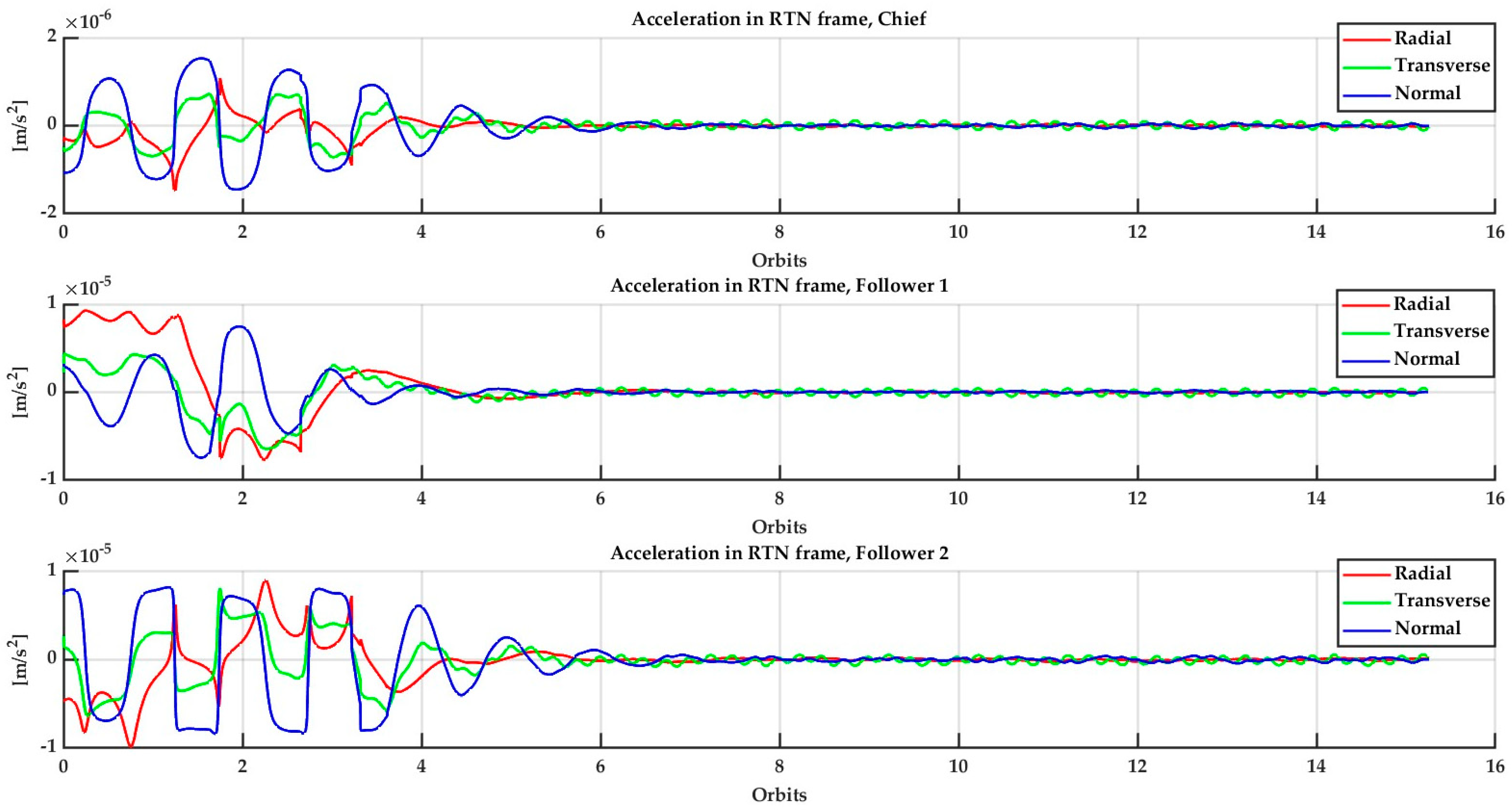
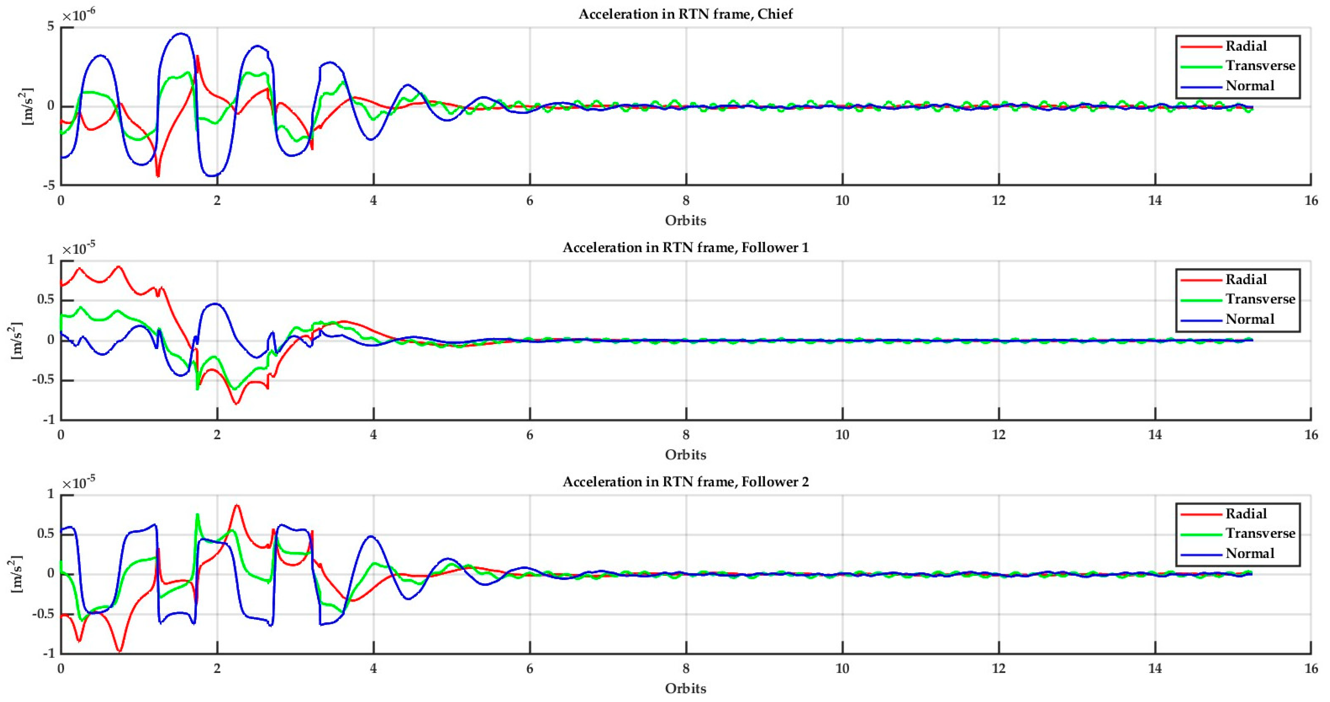
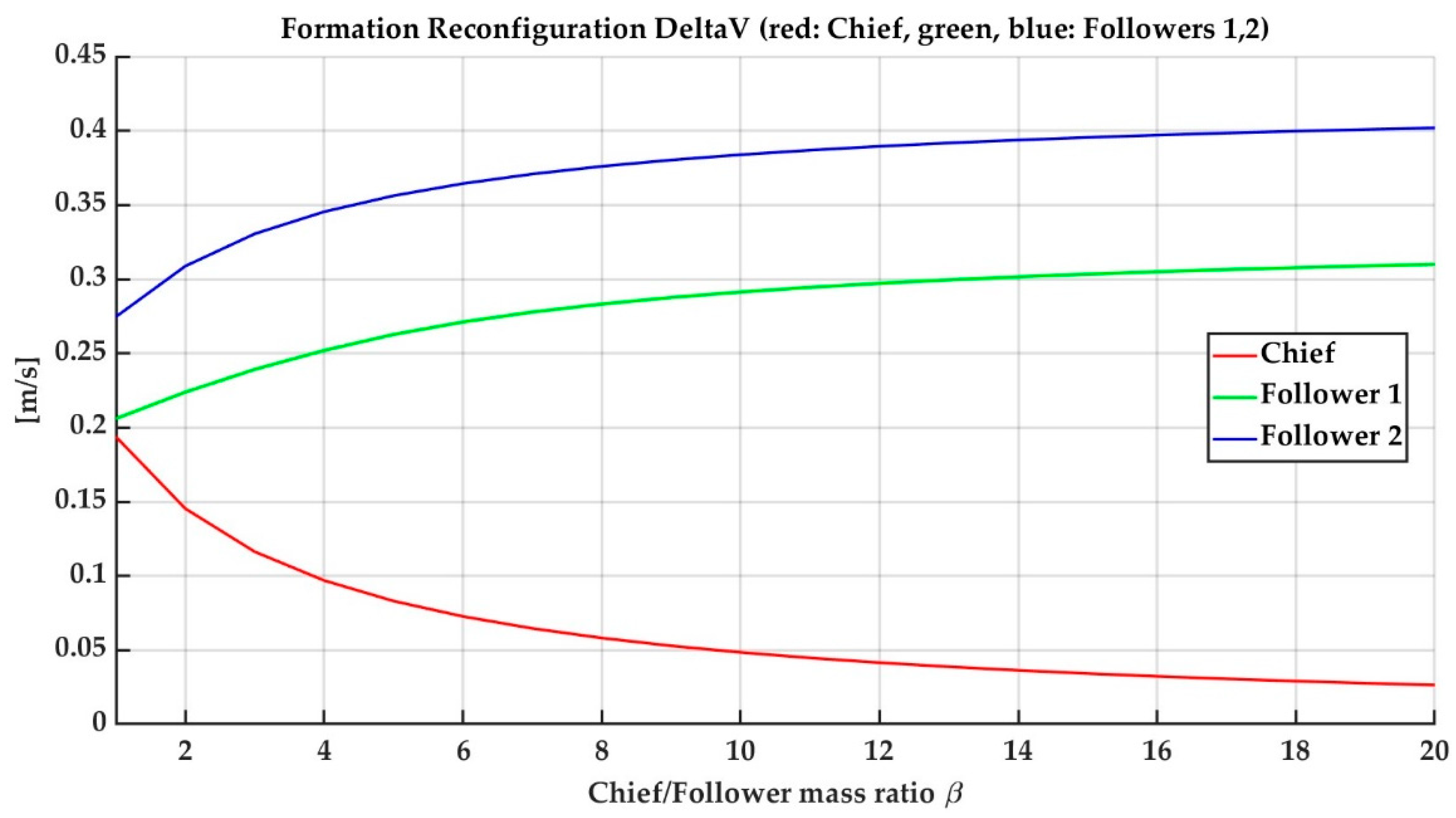
Figure 11 and Figure 12 show the control acceleration evolution to implement the same formation reconfiguration as proposed for AT-InSAR, with $\beta =2$and $\beta =10$respectively. It is a verified fact that for a larger value of $\beta$, the control authority required on the chief becomes reduced in comparison with the followers’. This also has an impact on the DeltaV of each satellite, as shown in Figure 13. This could be taken for a trade-off on the specific constellation/formation system design under the particular restrictions and mission objectives, which is beyond the scope of this work.

Finally, note that the implementation of this distributed control requires knowledge of the satellite masses, which are time-varying; one of the main uncertainties in knowing the satellite mass which is given by the propellant consumption. However, by using very high specific impulse electric propulsion of several thousands of seconds, this becomes negligible. The feasibility of this specific impulse level can be verified with the Field Emission Electric Propulsion (FEEP) technology, which is available now as Commercial Off-The-Shelf (COTS) products for small satellites (see [38,39]).

In order to simplify the implementation of the saturation, the saturation on the control acceleration differences is defined as follows:

$$\Delta {\underset{\_}{a}}_{1R}=sat\left({\underset{\_}{a}}_{1R} -{\underset{\_}{a}}_{0R}\right)$$

(21)

$$\Delta {\underset{\_}{a}}_{2R}=sat\left({\underset{\_}{a}}_{2R} -{\underset{\_}{a}}_{0R}\right)$$

(22)

Therefore, it can be found that under previous assumptions and two followers:

$${\underset{\_}{a}}_{1R}=\Delta {\underset{\_}{a}}_{1R}\cdot \left(1-\frac{1}{\beta +2}\right)+\Delta {\underset{\_}{a}}_{2R}\cdot \left(-\frac{1}{\beta +2}\right)$$

(23)

$${\underset{\_}{a}}_{2R}=\Delta {\underset{\_}{a}}_{2R}\cdot \left(1-\frac{1}{\beta +2}\right)+\Delta {\underset{\_}{a}}_{1R}\cdot \left(-\frac{1}{\beta +2}\right)$$

(24)

$${\underset{\_}{a}}_{0R}=\frac{-1}{\beta +2}\left(\Delta {\underset{\_}{a}}_{1R}+\Delta {\underset{\_}{a}}_{2R}\right)$$

(25)

There is no real actuator saturation in (21) and (22), as the saturation is applied here to a difference between control accelerations on different satellites. However, one could use an estimate of the upper bounds on these maximum available differences, considering the margin to guarantee that the real actuator on the full expressions (15)–(17) does not reach any saturation limit.

6. Conclusions and Future Research

Autonomous orbit maintenance paves the way for Trusted Autonomous Satellite Operations (TASO) to become a reality in Distributed Satellite Systems (DSS). Here it is shown that TASO is attainable with low-thrust electric propulsion for two main objectives: achieve and maintain the satellite orbit on the constellation, using absolute orbit navigation, and on the formation, using a more precise relative orbit navigation. In this way, there is a dedicated navigation type for each Autonomous Orbit Control objective.

As a case study, we considered a DSS mission for Maritime Domain Awareness (MDA) using Distributed Synthetic Aperture Radar (SAR) instruments. We showed a formation geometry capable of tracking ship movements using single-pass Along-Track SAR Interferometry (AT-InSAR). In particular, we have proposed a single pass and multi-baseline implementation using a safe three-satellite formation, which allows us to avoid temporal decorrelation and to have different velocity scales to track simultaneously. In order to improve the repeatability of these SAR products, we have proposed a constellation of these formations. As we demonstrated, this can be solved by autonomous orbit control using low thrusts compatible with electric propulsion. A particular formation mass distribution was analyzed on which there is a chief whose mass is equal or greater than the mass of the followers by certain common factor. It was shown that for the combined formation/constellation control, the relative importance of the control authority (in terms of maneuver total Delta V) of the chief decreases in relation to the equivalent figure for the followers, as this mass ratio increases.

A Constellation of Formations approach was proposed as a way to model the problem, and the solution’s concept has been determined. The approach is based on the concept of a system of particles to describe each of the formations in the constellation in such a way that the relative control within the formation determines the Formation Flying, while there is a separate constellation control objective stated in terms of the center of mass of each formation, i.e., a constellation of formation’s center of masses. Both objectives were solved with the same feedback control law structure using relative orbital elements obtained from the mean orbit elements of each of the spacecrafts. This requires an inter-satellite communication link between the satellites on the same formation for the Formation Flying feedback computation and the knowledge of the constellation objective in terms of mean orbital elements for the constellation feedback computation, which may be obtained onboard by the desired orbit propagation.

Finally, notice that with the recent evolution of inter-satellite communications, it is possible to augment this Inter Satellite Link (ISL) capacity in order to share also the SAR data information in order to generate the interferogram onboard and, therefore, deliver it in near real-time to the user. In this way, as distributed satellite system solutions become more readily available, a concept of operation with onboard single pass multibaseline interferometry computation will make it possible to deliver high-quality SAR data products faster to the user for effective maritime monitoring.

Additional work must be addressed to perform more realistic simulations, including hardware in the loop to test Global Navigation Satellite System (GNSS) navigation hardware, control nonlinearities, and possible inter-satellite links topologies, in order to complete the mission concept at the flight segment system level.