Article

Prediction of Tail-Off Pressure Peak Anomaly on Small-Scale Rocket Motors

1
Alma Propulsion Laboratory, Department of Industrial Engineering (DIN), University of Bologna, 47122 Forlì, Italy
2
ASI, 00133 Rome, Italy
3
AVIO, Colleferro, 00034 Rome, Italy
*
Author to whom correspondence should be addressed.
Aerospace 2023, 10(2), 169; https://doi.org/10.3390/aerospace10020169
Submission received: 31 December 2022 / Revised: 7 February 2023 / Accepted: 9 February 2023 / Published: 13 February 2023
(This article belongs to the Special Issue Aerospace Combustion Engineering)

Abstract

:
Numerical studies intended to predict solid rocket motors anomalies are the major contributors when developing strategies to both limit expensive fire tests and to investigate and understand the physical phenomena from which anomalies can arise. This paper aims to present a mathematical–physical method to evaluate the pressure peak, namely Friedman Curl, occurring at the tail-off phase of small-scale rocket motors. Such phenomenon is linked to the grain solid particles arrangement (i.e., packing effect); indeed, those particles show a tendency to accumulate at a certain distance from the metallic case, implying a local burn rate increment and a combustion chamber pressure rise close to the tail-off phase. Comparisons between experimental and simulated combustion chamber pressure profiles are outlined to prove the effectiveness of the mathematical–physical approach. Simulations were carried out with an internal ballistic simulation tool developed by the authors of this work.

1. Introduction

In the current time frame, solid rocket motors have an active role in boosting phases, initial stages or embarked systems. The most important factors to be considered in the design of solid rocket motors are cost-effectiveness, the reliability of such technology, the capability of a high thrust-to-weight ratio and the high propellant density. More in detail, concerning the above-mentioned cost-effectiveness, the modern solid rocket design approach is mainly based on the use of numerical tools in order to estimate the solid rocket motors’ performance by eventually reducing the cost of expensive fire tests. One crucial performance parameter regarding the combustion chamber behavior within a solid motor is represented by the combustion chamber pressure profile [1], affected by numerous phenomena [2,3,4] (Figure 1a), some of which have been investigated by the authors of the present paper [5,6,7]. It consists of three main phases [8]: ignition transient (Figure 1b), quasi-steady state phase (Figure 1c) and tail-off (Figure 1d). Two of them (ignition transient and tail-off) are time-dependent transient phases; indeed, they are respectively affected by the combustion gas filling/emptying of the combustion chamber. Since those two phases influence the beginning and the end of the combustion, they are very much bounded in time (each phase occupies 5% of the entire pressure profile at most). On the other hand, a quasi-steady state phase implies a quasi-steady balance between the mass flow rate coming from the grain combustion and the mass flow rate exhausted by the nozzle. It involves 85–90% of the entire grain combustion duration [1].
However, it must be highlighted that the pressure curve depicted in Figure 1 may display a pressure spike near the burn-out, commonly referred to as the Friedman Curl [9,10] (also stressed in Figure 2b). Its occurrence is caused by an increment of combustion gas mass flow rate as the burning surface approaches the motor case.
The rise of mass flow rate is essentially due to an increase in the burn rate close to the wall because of a local heat accumulation. Such heat accumulation, which occurs during combustion, is produced by an uneven grain solid particles distribution close to the wall [9]. In fact, the bulk statistical distribution of the particles cannot be maintained at the wall because the wall acts like an infinite particle during propellant casting. More precisely, the propellant formulation at the wall shows a higher content of oxidizer particles immediately away from the boundary, regardless of the casting time [9,10]. In fact, due to the high shear stresses at the wall, solid particles show a tendency to migrate in a region with lower stresses, namely at a certain distance from the case [11]. Hence, grain thermal conductivity reduction occurs across an oxidizer particles-rich zone since the oxidizer-rich region has a lower thermal conductivity than the grain in its standard composition, as a result of the oxidizer’s low thermal conductivity. Thus, the heat flux across the propellant is restrained next to the case by the thermal insulation because of such change of conductivity, causing the local heat accumulation responsible for the burn rate rise. Scientific literature shows that the burn rate increment reaches up to 5 % of the nominal value. Furthermore, the size of the Friedman Curl pressure peak is affected by the kind of casting process performed to fill the motor case [11]. If the motor is firstly loaded with the composite propellant, and then the desired grain geometry is obtained by pushing a mandrel into the case, the Friedman Curl pressure peak turns out to be more evident on experimental pressure profiles [11,12]. Conversely, if the propellant shape is achieved with the mandrel already in position, the pressure spike is negligible. In fact, pushing the mandrel into the case implies an HTPB-rich flow close to the wall due to the propellant’s ascending motion; the flow composition in terms of HTPB near the wall is then homogeneous along the entire motor axis. On the contrary, when the casting is performed with the mandrel already in position, other factors, such as, for instance, the number and position of casting inlets, cause the propellant flow to be less homogenous in terms of its composition near the wall than the previously mentioned condition.
Because of the importance of obtaining accurate simulations [13], as previously mentioned, the Friedman Curl pressure peak must be modeled and estimated. Furthermore, in this work, small-scale solid motors are considered since such phenomenon is even more evident when they are involved. Such motors are often used to establish the average burn rate originated from a certain propellant composition [14]; thus, predicting the Friedman Curl effect can lead to the compensation of its effect on the mean regression rate. Those motors—whose pressure profiles are shown in Figure 2—usually consist of an aluminum/steel case and a cylindrical-shaped grain directly attached to the case itself without any liner or thermal protections between them. Because of that, small scale motors represent a straightforward case to begin considering, as no other phenomenon (such as the ablation of thermal protection material, or the thermal conduction through the liner) is involved.
The following work essentially includes three steps. First, propellant solid particles non-homogeneity is investigated close to the wall in order to carry out an estimation of the mixture concentration regarding each component of the grain. Second, the previously mentioned concentration is used to determine the density and thermal properties (i.e., thermal conductivity, specific heat) discrepancy next to the case with respect to the propellant in its standard composition (sufficiently far from the wall). Subsequently, the effect of such changes in a propellant standard composition is evaluated with respect to the standard regression rate. Third, an internal ballistics simulation tool, namely ROBOOST (rocket boost simulation tool) [15], developed by the authors of the present work, is employed to compute the influence of the Friedman Curl on solid motors ballistics by estimating the combustion chamber pressure profiles varying with combustion time. Finally, the simulated pressure curves and experimental data are compared and discussed.

2. Code Overview

The Friedman Curl pressure peak depends on the combination of different phenomena as explained before, such as solid particles mass concentration next to the case wall (Section 2.1), heat accumulation during combustion while the burning surface is approaching the case (Section 2.2) and the combustion chamber internal ballistics (Section 2.3).

2.1. Particle Packing Model

In order to understand the packing structure, and therefore the particle distribution, of a powder-based material, a sphere packing study must be performed. The model that was set up for this work considers spherical particles, each of them characterized by their radius. If the propellant had monodispersed particles, the radius was considered to be the same for all the spheres; if the propellant had bi-dispersed or poly-dispersed particles, the spheres were divided into groups (species), each of them characterized by the same radius. This assumption gives a simplified representation of a real propellant, in which particles of the different species do not share the same radius, but rather a randomly distributed radius around the average value, which is considered constant in this work. Despite this simplified assumption, the results are considered representative of the real packing, as also reported by other works on the same topic [16,17,18,19]. The ratios among the radius values are considered the main parameter that identifies the packing problem, and, for simulation purposes, the dimensions of the different particles are normalized with respect to the largest ones, so that they are always lower than one.
The particle packing of each propellant was obtained considering a number of particles of each species such that the volumetric proportion among them was maintained. In order to ensure a good significance of the results for the distribution of each species, a minimum number of particles for each species was considered in relation to the characteristic dimension of the simulated domain [20]. A consequence of these assumptions is the possibly very large number of spheres to be managed if the radius ratio of the different species is high and the volume fraction of the small particles is relatively high. In this case, indeed, the minimum number of large spheres enforces a very high number of the small ones. While a large number of particles provides a better representation of the packing problem, it also requires a very large computational effort and a lot of time. To reduce this effort, the maximum total number of spheres considered acceptable for this work was set at 10 6 . All these considerations were included while dimensioning the simulation domain and the spheres distribution.
The packing model uses the volume fraction and the radius of the different species as inputs and, based on the previous considerations on the minimum significant number of particles per each species and the relative radius ratios, a total number of particles was chosen. The shape of the domain was designed as a cube whose volume is 1.2 times the total volume of the particles.
Periodic boundary conditions in the three directions of the cube can be set if the undisturbed packing has to be determined, while wall-bound conditions will be considered on one direction if the effect of the walls on the packing structure and local propellant composition is to be studied.
Once the domain was dimensioned, the initial position of each sphere was randomly assigned within it. Each i -th particle could then be identified by the following set of parameters, i.e., radius and position vector (Equation (1)):
r i ,   x 1 i ,   x 2 i ,   x 3 i
The choice of the domain volume (1.2 times the total volume of the particles, as mentioned before) does not usually guarantee that all the particles may be accommodated. In addition, each sphere was randomly placed in the simulation domain, likely generating an impossible packing (as some of them overlap). To solve this overlap, a collective rearrangement algorithm was applied: this process, based on the evaluation of the repulsion forces generated by the sphere overlap, iteratively moves each particle in the direction of the applied force until all the intersections are removed [21].
The repulsion force generated by the overlap of two spheres can be evaluated according to Hertz theory as (Equation (2)):
F i j = k p r i j   δ i j   n i j
where r i j = r i   r j r i + r j is the average radius, k p is the material stiffness, δ i j = || X i X j || r i r j is the overlapping distance and n i j is the normal vector in the direction of the connecting line between the two spheres. Since a sphere can overlap with multiple spheres, the resulting force on each sphere is the sum of all the forces (Equation (3)):
F i = j k p r i j   δ i j   n i j
Once the total force is computed, the sphere motion is evaluated as (Equation (4)):
Δ X i = k v F i r i 3
Clearly, k v strongly influences the convergence speed and the stability of the algorithm. After a “tuning” phase, the final value for this parameter is set as (Equation (5)):
k v = m i n 100 ,   1 + r i 3 δ i j   m a x
As already mentioned, the periodic boundary conditions were set to simulate the packing condition in a region far from the tank walls, while a wall boundary condition was used to simulate the packing condition close to a wall. If a wall boundary condition is active, every time a particle crosses the boundary of the domain, an additional force (Equation (6)) is considered on the particle:
W i = k w r i   δ i   n i
and the motion of the sphere is evaluated as (Equation (7)):
Δ X i = k v W i + F i r i 3
Every time the collective rearrangement procedure is activated, the reduction of the spheres overlapping is checked via the evaluation of the sum of all the overlaps among the spheres with Equation (8).
δ = i j δ i j
The collective rearrangement procedure was repeated until the value of δ did not improve anymore. This can happen either because δ reaches a value equal to zero (case 1—no more interactions), or because it reaches an asymptotic positive value (case 2—still interactions that cannot be improved by simply moving the particles). In case 1, the domain volume is overestimated with respect to the minimum one capable of containing the total number of particles; in case 2, the domain volume is underestimated. The following step is a contraction of the simulation domain in case 1, and an enlargement of the domain in case 2. This procedure is performed by proportionally moving by a factor k f both the positions of the sphere centers and of the boundaries ( k f < 1 in case 1, while k f > 1 in case 2).
Once the new positions were determined, the collective rearrangement procedure was started again and repeated until the asymptotic condition on δ was reached. This loop was repeated a number of times N m a x that can be chosen to be high enough to ensure that the minimum volume condition was obtained, as shown in Figure 3 below, which describes the algorithm flowchart.
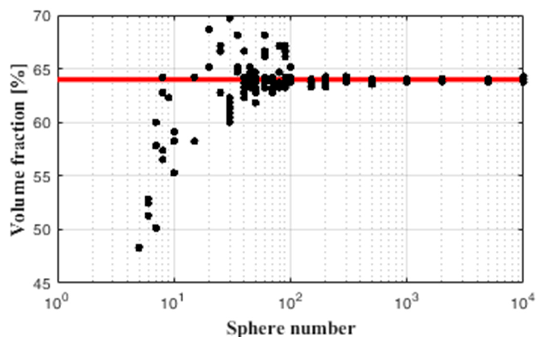
Validation of the packing model has been performed obtaining the results of the algorithm for a monodispersed set of particles within a domain with periodic boundary conditions applied in all the directions. As is well known from the literature, the expected particle volume fraction of a random close packing (RCP) algorithm for this type of simulation is equal to 64% [22,23,24]. Random close packing (RCP) models are extensively used to study the composition limits of a solid propellant, checking that the amount of the liquid component is higher than the empty volume available in a theoretical packing of the solid particles. Within real propellant systems, solid particles will not be as close as the positioning determined by RCP. Nonetheless, the amount of liquid component that is additional with respect to the minimum amount required to fill the gaps among the particles is limited (to keep the ballistic performance high) and therefore the particle positioning will still be well represented by an RCP model. Figure 4 shows the particle volume fraction evaluation that was obtained with the algorithm described in the previous paragraphs, as a function of the number of spheres involved in the process.
As it can be seen from Figure 4, the algorithm is capable of correctly estimating the expected volume fraction for an RCP, if the minimum number of spheres involved in the procedure is higher than 100. Figure 4 shows also a rising value of the volume fraction as the number of spheres increases. This is due to the fact that the packing procedure tries to keep the spheres within a cube: periodic conditions become effective only if the number of spheres is high. 
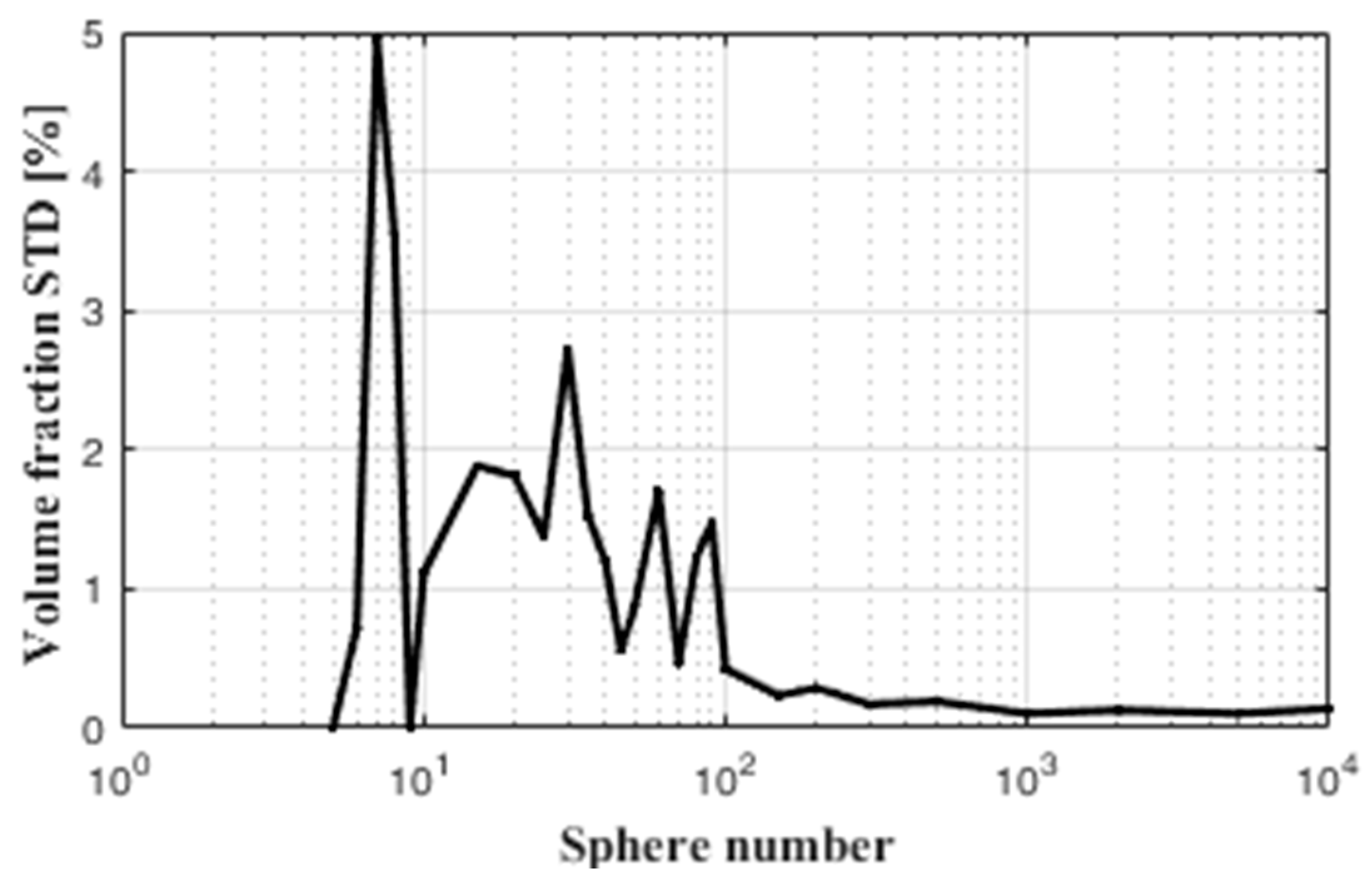
Figure 5 reports the standard deviation that has been computed for the volume fraction obtained by repeating the procedure 10 times for each number of spheres considered, using different initial random placements of the sphere centers. Once again, it can be stated that if the number of spheres involved in the procedure is higher than 100, the packing model can provide significant results.
Figure 6 shows the final position for a packing of 2000 monodispersed spheres of a radius equal to 1, applying periodic boundary conditions in all directions and obtaining a volume fraction of 64%.

2.2. Grain Heat Propagation

Figure 7 shows the mathematical–physical domain used to describe the heat propagation in this work. The dark yellow cylinder (with one annulus at each base) in the upper part of the figure represents the solid rocket motor burning surface which, during combustion, approaches the metallic case (the gray cylinder). The domain over which the heat propagation model was defined is shown in the same figure (enclosed in the red square). More in detail, given the spatial direction r along the motor radius, the grain region is included in the range R 1 , R 2   , where R 1 and R 2 are, respectively, the minimum and maximum radius of the motor grain; on the other hand, the case is defined by r R 2 , R 2 + t c , where t c is the metallic case thickness. Once ignited, the burning surface advances toward the case and along the direction of a quantity s , defined with respect to the reference coordinate R 1 . Then, at a generic time instant t , the burning surface position with respect to the origin O (the reference frame is identified by the coordinates z and r ) is r b s t (or equivalently R 1 + s t ). Additionally, during burning surface advancement, a certain amount of grain (of s t ) is burned, producing combustion chamber hot gas, which contributes to maintaining the combustion chamber temperature at a constant level ( T g a s ).
Three heat transfer phenomena are considered across the burning surface. Two of them, namely radiation ( q ˙ r a d , i.e., radiative power) and convection ( q ˙ c o n v ) involve the heat flux coming from the combustion gaseous products in the motor chamber; on the contrary, conduction ( q ˙ c o n d ,   i . e . ,   conductive   power ) concerns the heat spreading through the grain/case sample. The heat produced by grain combustion is assumed to spread across the solid propellant driven by the following form of the heat equation (Equation (9)):
T t = 1 ρ c r r k r T r ,
where T is the temperature. Furthermore, ρ , c and k represent the density, specific heat and thermal conductivity of the material sample (grain or metallic case, as shown in Figure 7), respectively.
Equation (1) relies on the following assumptions [25]:
  • Temperature T varies with respect to time t and direction r , and it is estimated only in the grain/case domain (i.e., r R 1 , R 2 + t c ).
  • The density, specific heat and thermal conductivity ( ρ , c and k ) vary with r (both due to the presence of grain and case material, and the different propellant composition near the case from the nominal concentration). In addition, the propellant temperature-dependent specific heat and thermal conductivity are also considered.
  • The solid phase reaction heat per unit time is assumed to be negligible in the equations [26]. However, such a hypothesis does not imply that the combustion reaction heat is not considered in the present model; as previously described, the heat exchange (convection and radiation) between the combustion chamber hot gas and the propellant is taken into account. Then, when the solid propellant gasifies, the hot gas produced by combustion reaches a temperature value that is also linked to the combustion reaction heat of the grain. Thus, it is sufficient to assume a coherent hot gas temperature (i.e., chamber equilibrium temperature) in order to include the temperature-increasing effect of the reaction heat.
  • The cylindrical coordinates ( z ,   r , and i θ , i.e., the perpendicular direction to the plane identified by the coordinates z and r ) are chosen instead of cartesian coordinates to obtain a consistent estimation of the heat spreading through an axisymmetric body (i.e., the grain circular geometry shown in the upper part of Figure 7). The reference frame is positioned at the center of the motor (Figure 7), where z is aligned with the motor axis; r and i θ are chosen on the plane orthogonal to z .
Additionally, Equation (9) requires two boundary conditions (Equations (10) and (11)) and one initial condition (Equation (12)).
q ˙ c o n v + q ˙ r a d = q ˙ c o n d
where:
q ˙ c o n v = h c T g a s T t , r = R 1 + s q ˙ r a d = σ ε g a s T g a s 4 T 4 t ,   r = R 1 + s q ˙ c o n d = k T ,   r = R 1 + s T r r = R 1 + s
T r r = R 2 + t c = 0
T t = 0 , r = T a m b
where h c and σ are, respectively, the convective heat transfer coefficient and the Stefan–Boltzmann constant.
Equation (2), Robin type, ensures the energy balance at the burning surface: convection ( q ˙ c o n v ) and radiation ( q ˙ r a d ) fluxes produced by combustion chamber hot gas are transferred through a conduction ( q ˙ c o n d ) process across the solid grain up to the metallic case. However, it must be highlighted that Equation (10) is a moving boundary condition: a dynamic heating process raises the burning surface temperature up to the grain surface temperature ( T a ); then, as previously mentioned, the solid propellant infinitesimal layer is burned, causing the advancement of the burning surface along direction r . For this reason, the burning surface temperature and its derivative and thermal conductivity are specified at the spatial coordinate r = R 1 + s (Figure 7), where s increases over time. Moreover, ε g a s identifies the combustion chamber gas emissivity. Since aluminum-base grain combustion often leads to the formation of alumina particles, Equation (13) has been involved. The above-mentioned empirical formula indeed represents the correlation of an optically thick cloud of particles (alumina) of uniform diameter ( D p ) immersed in the combustion products [27,28].
ε g a s = 0.17 + 0.22 T g a s 1000 0.87 0.1 T g a s 1000 e 0.11 D p T g a s 1000
The second boundary condition (Equation (11), Neumann type) is set at the end of the case ( r = R 2 + t c , see Figure 7) and specifies the amount of power exchanged between the case and the external environment. In the present work, a case adiabatic condition applies. Regarding the initial condition (Equation (12)), the ambient temperature ( T a m b ) is assumed to be constant in the entire domain at the initial time instant t = 0 s.
Another important aspect to deal with is the grain combustion phenomenon. Typically [26], the grain combustion process is modelled through the formation of three different zones (heterogeneous model, Figure 8), each one linked to a specific thermal condition. Concerning the three layers, starting from the unburned propellant side, a first solid region is present where high exothermic reactions induce the grain constituents’ degradation. Closer to the burning surface is a second layer consisting of a two-phase mixture of melted liquid propellant and combustion reaction products (sub-surface liquid region, Figure 8). The third layer is gaseous phase-dominant incorporating the most of the evaporated species coming from the decomposition of the grain ingredients (gas phase, Figure 8). Such an approach is named a heterogeneous model, since, as previously outlined, all three matter phases are included. Despite its great accuracy in terms of combustion physical consistency, the above-mentioned model implies high computational time efforts due to its complexity, which is also increased by the need for tracking all the chemical compounds’ concentrations within the domain [26].
Hence, to reduce computational effort, combustion was assumed to be an instantaneous propellant gasification (Equation (14), Figure 8) once the propellant reaches a temperature higher than its activation temperature ( T a ).
T = T , T < T a T g a s , T T a
Immediately after its formation, gaseous combustion products are supposed to instantaneously reach the combustion chamber equilibrium temperature. In such a way, the liquid and gas phases are neglected, allowing only the solid grain/case temperature distribution to be computed; no time/spatial gas temperature variations in the combustion chamber are considered (region within the range r 0 , r b s   in Figure 7).
Additionally, the burn rate is estimated as the first order derivative of the burning surface position ( s ) with respect to time t (Equation (15)).
r b = d r b s d t = d s d t
Equations (1) to (7) define the heat equation model, whose solution flowchart procedure is shown in Figure 9.
The experimental values of the convective heat transfer coefficient are not available: therefore, an iterative procedure has been developed with the aim of estimating the previously mentioned parameter. First, after a proper initialization of the grain’s thermo-chemical properties (composition, density, specific heat, thermal conductivity, surface temperature, initial temperature, combustion chamber temperature and alumina particles diameter), an initial value of the coefficient ( h c g u e s s ) is assumed. Secondly, the heat equation model is solved numerically, obtaining the computation of an average value of the burn rate, namely r b , r e f (Equation (15)). Thirdly, the simulated burn rate (Figure 9), i.e., r b , r e f , is compared to the experimental mean burn rate r b , e x p (obtained from the experimental data, Figure 9). If their difference is lower than a user-defined tolerance ε , then value h c adopted at step one is accepted. On the contrary, if r b , r e f does not match with r b , e x p , the entire procedure is repeated until there is a convergence. However, in the interest of validating the physical consistency of the obtained values of h c , they are compared to the ones obtained through the following empirical formula (Equation (16), [25]):
h c = μ c p · N u P r · D h
where:
N u = 0.023 · R e d 0.8 · P r 0.4
where almost all quantities refer to the combustion chamber’s hot gas: μ , c p , N u , P r and R e d are the dynamic viscosity, constant pressure specific heat, Nusselt number, Prandtl number and Reynolds number, respectively. On the contrary, the hydraulic diameter D h is linked to the combustion chamber propellant geometry. Since the flow within the combustion chamber of solid rocket motors is highly turbulent, Dittus–Boelter’s correlation (Equation (16)) for a fully developed turbulent flow in a smooth pipe is widely accepted. The following assumptions are accepted. First, the flow is considered steady since the convective heat transfer time-dependent effects are negligible [29]. Second, the propellant surface roughness effect, which increases the heat transfer to the surface, is balanced by the decomposition-gasification of the unburned propellant surface, which attenuates the heat transfer process. Third, because grain combustion has been modeled as an instantaneous propellant gasification, no sharp variation of the fluid properties occurs across the boundary layer, which has a negligible thickness. Furthermore, no heat-releasing/heat-absorbing processes like exothermic/endothermic chemical reactions take place on the grain surface.
In general, the solution of the heat equation model requires discretization in time and space by dividing the entire domain in a certain number of spatial nodes. Nevertheless, as previously mentioned, the burning surface (and its moving boundary condition, i.e., Equation (10)) recedes in time along direction r during the combustion process, meaning that at each time instant, one or more spatial nodes of the domain should be dropped since they are linked to the burned propellant converted into combustion chamber gas. From a numerical perspective, this implies a time-variant spatial grid, which depends both on the chosen time/spatial step and the burn rate entity. In fact, if both the time and spatial step are not chosen small enough to be consistent with the estimated burn rate, severe instabilities could arise. Such instabilities could even be worsened by the spatial node dropping process previously described. These issues can be avoided by introducing the following coordinates transformation [30]:
η = β r R 1 s
where:
β = 1 R 2 R 1 s
In this way, the spatial grid, now expressed in terms of coordinate η , is constant in time, and both boundaries are fixed at η = 0 (burning surface) and η = 1 (end of the grain, i.e., r = R 2 ). The previous coordinates transformation is applied to the heat equation model equations regarding only the propellant part of the domain ( r R 1 + s ,   R 2 , Figure 7). Consequently, Equations (9) and (10) become Equations (18) and (19), respectively:
q ˙ c o n v + q ˙ r a d = q ˙ c o n d
where:
q ˙ c o n v = h c T g a s T t , η = 0 q ˙ r a d = σ ε g a s T g a s 4 T 4 t , η = 0 q ˙ c o n d = k T ,   η = 0 β T   η   η = 0
1 β 2 T t = s ˙ β 1 η T η + 1 c ρ η + β R 1 + s η k η + β R 1 + s T η
where:
s ˙ = r b = d s d t
It must be pointed out that the coordinate transformation (Equation (17)) was also applied to Equation (10), since that boundary condition refers to the propellant part of the domain as well.
On the contrary, the heat equation model specified for the case part of the domain ( r R 2 ,   R 2 + t c ) including the boundary condition (Equation (11)) imposed at the case-external environment interface, is still formulated in cylindrical coordinates (Equations (20) and (21)) since no material depletion occurs in that region.
T t = 1 ρ c c c r r k c r T r
T r r = R 2 + t c = 0
where ρ c , c c and k c are the density, specific heat and thermal conductivity of the case material, respectively.
To ensure the continuity and the derivability of the temperature function at the interface between the propellant and the case ( r = R 2 or η = 1 ), the following relations are assumed (Equation (22) is linked to the continuity, Equation (23) to the derivability):
T t , η = 1 = T t ,   r = R 2
k T ,   η = 1 β T η η = 1 = k c T r r = R 2
Hereinafter, the heat model refers to Equations from (18) to (23). After the unknown functions computation ( T and r b ) in the coordinates θ ,   η , it is sufficient to apply the inverse of the transformation established with Equation (17) to obtain them, formulated with the coordinates r ,   t .
The numerical technique used to achieve the solution of the heat equation model is the finite difference method [31]. More in detail, spatial derivatives are discretized with a three-point stencil (2nd order accuracy) using a centered scheme; time derivatives rely on the backward Euler scheme (1st order accuracy). The time step selected is d θ = 1 · 10 3   s ; the spatial step d η choice will be discussed in the Results section.

2.3. Combustion Chamber Internal Ballistics

The internal ballistics evolution within the motor combustion chamber is estimated by means of ROBOOST (rocket boost simulation tool), an in-house software [15] developed in a MATLAB environment. It essentially consists of two interconnected main modules: a grain regression module and a ballistics module. First, the grain regression module is based on the adoption of a 3D triangular mesh regarding the discretization of the burning surface aimed at guaranteeing the ability to handle generic geometric shapes, accepting CAD file formats as inputs. Moreover, the regression of each mesh node is managed independently from the others, thus making the application of a specific burn rate possible; thus, it gives the opportunity to insert both defects (like air inclusions [6,15] and/or propellant debondings [5,32]) and inhomogeneities (like the burn rate variation responsible for the Friedman Curl pressure peak) into the grain. Secondly, the ballistics module consists of a 1D fluid-dynamics model [32] describing the evolution of the combustion chamber flow. The equations system is solved by applying a finite difference discretization approach for both spatial and time-related derivatives. The two above-mentioned modules are mutually coupled: at the present time instant, the grain regression module evaluates the propellant mass flow rate burned. Then, together with the thermodynamic parameters carried out through the ballistics module, a new burn rate value is computed for each mesh node, implying new nodes spatial positions at a new time instant. If the remaining propellant volume at the new time instant is below a certain user-defined tolerance with respect to the remaining propellant volume obtained at the present time instant, then the code moves to the next iteration; otherwise, the entire procedure is repeated until convergence is achieved.
As previously outlined, the Friedman Curl pressure peaks originate from burn rate variations, with respect to the nominal one, close to the case wall. In order to include the phenomenon, the nominal burn rate (expressed by means of the widely used Vieille law, Equation (24)) is multiplied by a coefficient φ . Such a coefficient is meant to act as a correction of the average burn rate and is defined as the ratio between the local burn rate (evaluated through the heat equation model) and the average one.
r b = a p 0 n · φ
where a , n and p 0 are, respectively, the burn rate experimental factor, the burn rate experimental exponent and the combustion chamber’s pressure. Since the length-to-diameter ratio of the considered small-scale motor is low, the erosive combustion effect has been neglected.
Finally, the new burn rate (i.e., the one including the above-mentioned φ correction) is coupled with the combustion chamber fluid-dynamics using Equation (25)
d V 0 d t = A b r b
where V 0 and A b are the combustion chamber volume and the area of the burning surface, respectively.

3. Results

The analysis outlined in Section 2 was performed on BARIA small-scale rocket motors (Figure 10) used for the composite propellant characterization. In this study, the small-scale motors considered were filled with a composite propellant identified by the composition HTPB-1814 [33], where the aluminum powder (fuel), ammonium perchlorate (oxidizer) and HTPB (Hydroxyl-Terminated-PolyButadiene, plastic binder) mass percentages were, respectively, 18 % , 68 % and 14 % . Such a grain composition has been used to investigate Ariane 5 booster behavior in subscale testing [33].
As previously mentioned, first each motor was filled with propellant; then, the circle-shaped grain geometry was obtained by means of a mandrel, which was pushed inside the motor at a constant velocity. At the interface between the case and the rising propellant flow, the high shear stresses induce most solid particles to migrate to a zone (corresponding to a low-stress region of the flow domain) at a certain distance from the wall, thus causing the rise of the Friedman Curl effect during combustion, as previously outlined. The solid particles migration phenomenon corresponds to a viscosity variation within the flow: lower viscosity occurs in the high-stress regions, and vice versa, higher viscosity appears in low-stress regions. This behavior corresponds, from a macroscopic perspective, to a non-Newtonian flow: a liquid composite propellant, indeed, can be regarded as very close to a shear-thinning fluid [34].
Several sets of BARIA were casted to determine the properties (consisting of Vielle law parameters a and n ) of each batch of propellant. In the present work, three sets of BARIA were considered (condition 1, condition 2 and condition 3 set, Figure 11), each one corresponding to the same propellant composition [11]. Each motor had the same dimensions (Figure 10) and weight except for the nozzle throat diameter. This parameter was different in each BARIA set in order to obtain different combustion chamber pressure/burn rate levels.
In Figure 11, each quantity, i.e., experimental burn rate ( r b , e x p ) and combustion chamber pressure ( p 0 ) are respectively nondimensionalized with the corresponding maximum values of the burn rate, pressure and time regarding the three BARIA sets.

3.1. Estimation of the Propellant Ingredients’ Concentration Close to the Wall

The packing model that was developed and presented in the previous sections was used to estimate the wall effect on the mass fraction of the different components of the propellant in the vicinity of the wall. To do this, the propellant was considered to be composed of a solid phase (powders of AP and Al) and a liquid one (HTPB).
The solid phase was included within the packing procedure, while the liquid phase was considered capable to completely fill the gaps available between the solid gaps. The particle sizes for AP and Al were such that the relative ratio among them was, on average, equal to 10, and for this reason, the packing model was initiated with a bi-dispersed particle distribution, with the larger spheres representing the AP particles and the smaller ones representing the Al particles. The simulation was run considering the wall boundary conditions on X direction and the periodic boundary conditions on the remaining directions (Y and Z). The number of particles considered was set at 150 for the larger ones and 16,667 for the smaller ones, in compliance with the observation on the minimum number of particles to be considered to obtain significant results from the simulations. The packing solution that was found for this simulation is reported in Figure 12.
From this packed distribution, the following step was completed to obtain the volume fraction occupied by each species of particles and the volume fraction that remained free for the liquid phase of the propellant during the manufacturing process. This was achieved considering the section of the particles on the planes that were orthogonal with respect to the x direction and computing the percentage of area in the section that was occupied by each species. As stated before, within real propellant systems, solid particles will not be as close as the positioning determined by RCP. The gaps between particles will be randomly distributed and not uniformly equal to zero. The effect of this random distribution is a smoothing of the sharp waveform representing the mass fraction of the different component. To take into account this effect, filtering was applied to the raw output of the RCP model. The result obtained is reported in Figure 13, both in terms of the raw evaluation (ref line) and its filtered version (black line). Filtering was applied as a moving average of the signal in order to smooth the peaks due to the sorted order that was established in the vicinity of the wall.
As can be noted, there was an increased presence of large spheres (which represent the AP particles) close to the wall, mainly due to the sorted order that occurred due to the presence of the boundary. This also caused a reduction of the mass fraction of the Al particles.
The outcome of this process is the percentual mass fraction of ammonium perchlorate ( N H 4 C l 0 4 ), aluminum powder ( A l ) and a plastic binder ( H T P B ) with a focus close to the wall.

3.2. Heat Equation Model Solution

Before introducing the results of the simulations, some information regarding the propellant’s thermal properties and the combustion chamber’s environment is required.
As already discussed, the propellant considered in this study is HTPB-1814. The densities of each grain component, i.e., N H 4 C l 0 4 , A l and H T P B , are, respectively, 2700   k g m 3 , 1950   k g m 3 and 920   k g m 3 . With respect to their mass fractions, a standard concentration ( N H 4 C l 0 4 : 68 % , A l : 18 % , H T P B : 14 % ) is observed in most of the propellant domain (from normalized r = 0.625 to nearly normalized r = 0.983 , Figure 13), except for the plastic binder, whose concentration is maintained equal to the nominal one. Moreover, the thermal conductivity ( k ) and specific heat ( c ) of ammonium perchlorate and Hydroxyl-Terminated-PolyButadiene were chosen as functions of the grain temperature T [35], as illustrated in Figure 14.
For the aluminum powder, a thermal conductivity of about 47   W m · K was used [36]; the aluminum powder, indeed, consisted of agglomerates (with a mean size of about 10   μ m ) of spherical particles with an average diameter of 0.1 0.3   μ m . The formation of an aluminum oxide layer on the particles’ surface implies a reduction in thermal conductivity, which results in a lower value than the one corresponding to regular aluminum ( 237   W m · K ). Furthermore, aluminum-specific heat of about 900   J k g · K was assumed. However, since the overall grain properties are required by the heat equation model, the propellant thermal conductivity and specific heat were carried out by means of a weighted average [37,38] of conductivity and specific heat corresponding to each component (as already mentioned, the temperature dependance characterizes both N H 4 C l 0 4 and A l ), where the weight coefficients refer to the grain ingredients’ mass fractions along direction r (Figure 13). The final outcome is two maps related to grain thermal conductivity and specific heat, both treated as functions of temperature T and spatial position r . Since conductivity is a measure of the power spread within the material, the difference between the nominal grain conductivity and the conductivity close to the wall, where the solid particles’ mass fraction varies (Figure 13), is the main reason for the heat accumulation rise next to the wall. The above-mentioned weighted average was performed for the grain density, which depends only on the spatial coordinate r . Other initialization parameters are initial grain temperature T a m b = 293.15   K and propellant surface temperature T a = 650   K [21].
On the other hand, concerning the combustion chamber environment, the hot gas temperature was about T g a s = 3300   K [1] and the alumina particles’ diameter (Equation (13)) was D p = 3   μ m [28,39].
Three simulations were performed, each one for one of the three burn rate conditions (Figure 11a). The entire procedure leading to the heat equation model solution consisted of three main steps. First, a pressure/burn rate level for the BARIA set was chosen (Figure 11a), for instance BARIA set at condition 1. Then, the average experimental burn rate ( r b , e x p ) was computed by averaging the experimental recession rates linked to that pressure condition (light blue dots in Figure 11a). This value was compared to the average simulated burn rate ( r b , r e f ) in order to obtain the corresponding value of the heat transfer coefficient, using the iterative algorithm described in Section 2.2 (Figure 10). Second, the heat equation model (Equation (18) to Equation (23)) was solved considering all the above-mentioned input data, up to the burn-out time ( t b ) when all the grain was completely depleted. Third, since the heat equation model unknowns, i.e., temperature T and burn rate r b , are expressed in the coordinates θ and η , Equation (17) was applied to refer them to coordinates t and r .
Figure 15 shows the heat equation model solution for the BARIA set at condition 1. More in detail, Figure 14a,b represents the burn rate profile along r direction. It must be noticed that in most of the domain, up to normalized r = 0.975 (Figure 11a), r b is constant due to the absence of the grain components’ concentration variation (Figure 13) with respect to the nominal one. It is indeed equal to the average value r b , r e f (black dotted line in Figure 15a,b), which represents the burn rate value in a standard combustion. However, close to the case (Figure 15b), because of heat accumulation caused by a different propellant composition, the burn rate starts to rise with a peak nearly at normalized r = 0.988 , where heat accumulation reaches its maximum amount. Then, the burn rate experiences a sudden fall (Figure 15a, close to normalized r = 0.994 ) since most of the heat produced by combustion was drained away by the metallic case, which, with a higher thermal conductivity than the propellant one, behaves as a heat sink.
Figure 15c,d display the grain temperature map varying with time t (nondimensionalized with burn-out time t b ) and in space ( r ). A maximum temperature equal to the surface temperature ( T a = 650   K ) was reached because, beyond that threshold, the grain is depleted and becomes combustion chamber hot gas at a high temperature ( T g a s = 3300   K ) (white region in the graphs of Figure 15c,d). It must be highlighted that the slope of the interface line between the colored region and the white one is linked to the burn rate, since, as already mentioned, it was computed as the time derivative of the spatial coordinate (Equation (15)). This implies a relation of inverse proportionality between the tangent of the angle, established by the interface line and r axis, and the burn rate. When the burn rate is constant (Figure 15a), the angle remains the same (Figure 15c, up to normalized r = 0.975 ) in coherence with burn rate behavior; on the contrary, when the angle slightly decreases (Figure 15d), the burn rate reaches its peak (Figure 15b). In the end, the angle quickly grows, causing a rapid descent of the burn rate (Figure 15b).
The r b profile was determined through the previously described procedure for all the three burn rate conditions (Figure 16b,c). All the initialization parameters were the same except for the convective heat transfer coefficient, which differs according to the pressure level. Although such values are not time-dependent, since they are computed matching each value of the mean burn rate of the three BARIA conditions, they adequately reproduce the heat transfer between the combustion chamber and the grain surface. It must be emphasized that a high convective heat transfer coefficient also corresponds to a high burning rate (Figure 16a), since a large amount of heat is transferred from the combustion chamber hot gas to the burning surface. In fact, for the same motor geometry, a large combustion chamber pressure causes a high velocity of the gas flow, implying an increase of the Reynolds number. Thus, according to Equation (16), the maximum convective heat transfer coefficient is linked to condition 1 (Figure 16a), i.e., the condition of maximum pressure and flow velocity. On the opposite hand, the minimum pressure condition identifies the lowest heat transfer coefficient value. This tendency is also present in the percentual burn rate increment with respect to the nominal one (Figure 16c): concerning the maximum burn rate condition (BARIA set at condition 1), the percentual increment of about 4 % is the highest, since the large amount of hot gas power spreading through the propellant implies the maximum amount of heat accumulation next to the wall. The opposite happens for the lowest burning rate condition, since the amount of heat accumulation is lower compared to the one of condition 1.

3.3. BARIA Combustion Chamber Pressure Results

After performing internal ballistics simulations for all the three pressure/burn rate conditions of the three BARIA set with ROBOOST software described in Section 2.3, a comparison between the simulation (colored curves, Figure 17) and the experimental data (light gray curves, Figure 17) was carried out. In Figure 17, the time and combustion chamber pressure p 0 have been nondimensionalized with the burn-out time and the maximum pressure taken from the experimental data, respectively.
A satisfactory overlapping can be noticed between the experimental Friedman Curl pressure peaks and the simulated ones for all the burn rate conditions (Figure 17b). This seems to suggest that, apart from the grain properties used as input data, the Friedman Curl pressure peak depends on the burn rate condition only. Additionally, the different peaks and shapes of the three burn rate increments near the wall (Figure 16c) adequately explain the different behavior of the pressure curves in Figure 17b: the highest burn rate increment (blue curve, Figure 16c) corresponds to a sharp Friedman Curl peak (blue curve, Figure 17b) in the pressure occurring for the condition 1 BARIA set; on the contrary, the lowest burn rate increment (yellow curve, Figure 16c) produces a smooth pressure peak (yellow curve, Figure 17b) for the condition 3 BARIA set.

3.4. Spatial Grid Convergence

The spatial grid analysis was computed to evaluate the numerical error of the heat equation model. As previously mentioned, such a model is solved along the space direction in the variable η , where the domain range consists of η 0 ,   1 . Figure 18 shows the behavior (blue curve) of the percentual relative error between the experimental average burn rate ( r b , e x p ) and the simulated one ( r b , r e f ), and the time needed for the simulation, both varying with the number of grid points ( N η ) chosen to discretize the range 0 ,   1 . Six tests were performed at N η = 250 ,   500 ,   750 ,   1000 ,   1250 ,   1500 . An error of 3.5 · 10 2   % corresponding to N η = 1000 ( d η = 0.001 ) was considered acceptable as a trade-off between solution accuracy and computation time.
All the simulations previously discussed were carried out with ROBOOST software installed on a computer with the following features: 16 Gb RAM, 7th generation Intel Core i7, 3.10 GHz CPU and NVIDIA Quadro M1200 graphic card. Each simulation lasted 3 h.

4. Conclusions

A mathematical–physical approach to predict the Friedman Curl pressure peak in the tail-off phase of small-scale solid rocket motors was presented, with the aim of offering a deeper insight into such phenomenon. The overall algorithm is based on the coupling among different influencing factors, such as the grain components’ concentration, the combustion chamber fluid-dynamics and the heat equation model, used to estimate the burn rate percentual variation induced by local heat accumulation. The final solution consists of time-varying combustion chamber pressure profiles, which have been obtained for three burn rate conditions of the BARIA small-scale motors, in order to prove the predictive capability of the model itself. The satisfactory overlap between the experimental and the simulated pressure data suggests that, although the model considered is one-dimensional in space, the procedure is very effective.

Author Contributions

Conceptualization, S.M., F.P., A.B., R.B. and B.B.; methodology, S.M., F.P., A.B., R.B. and B.B.; validation, S.M., F.P., A.B., R.B. and B.B.; writing, S.M., F.P., A.B., R.B. and B.B.; supervision, F.P. and B.B. All authors have read and agreed to the published version of the manuscript.

Funding

This research received no external funding.

Data Availability Statement

Restrictions apply to the availability of these data. Data was obtained from AVIO spa and are available from B.B. with the permission of AVIO.

Conflicts of Interest

The authors declare no conflict of interest.

References

  1. Hill, P.G.; Peterson, C.R. Mechanics and Thermodynamics of Propulsion, 2nd ed.; Addison-Wesley: Boston, MA, USA, 1992. [Google Scholar]
  2. Baum, J.D.; Levine, J.N.; Lovine, R.L. Pulse-Triggered Instability in Solid Rocket Motors. AIAA J. 1984, 22, 1413–1419. [Google Scholar] [CrossRef]
  3. Yamada, K.; Goto, M.; Ishikawa, N. Simulative Study on the Erosive Burning of Solid Rocket Motors. AIAA J. 1976, 14, 1170–1176. [Google Scholar] [CrossRef]
  4. Hart, R.W.; Bird, J.F.; Cantrell, R.H.; McClure, F.T. Nonlinear Effects in Instability of Solid-Propellant Rocket Motors. AIAA J. 1964, 2, 1270–1273. [Google Scholar] [CrossRef]
  5. Mini, S.; Ponti, F.; Annovazzi, A.; Ravaglioli, V.; Moro, D. A Novel Procedure to Determine the Effects of Debonding on Case Exposure of Solid Rocket Motors. Acta Astronaut. 2022, 190, 30–47. [Google Scholar] [CrossRef]
  6. Ponti, F.; Mini, S.; Fadigati, L.; Ravaglioli, V.; Annovazzi, A.; Garreffa, V. Effects of Inclusions on the Performance of a Solid Rocket Motor. Acta Astronaut. 2021, 189, 283–297. [Google Scholar] [CrossRef]
  7. Ponti, F.; Mini, S.; Fadigati, L.; Annovazzi, A.; Corti, E. Influence of Nozzle Radiation on Solid Rocket Motors Tail-Off Thrust. Int. J. Energ. Mater. Chem. Propuls. 2021, 20, 45–64. [Google Scholar] [CrossRef]
  8. Sutton, G.; Biblarz, O. Rocket Propulsion Elements, 9th ed.; John Wiley & Sons: Hoboken, NJ, USA, 2016. [Google Scholar]
  9. Fry, R.S. Solid Propellant Subscale Burning Rate Analysis Methods Fo U.S. and Selcted NATO Facilities; Chemical Propulsion Information Agency: Columbia, MD, USA, 2002. [Google Scholar]
  10. Fry, R.S. Solid Propellant Test Motor Scaling; Chemical Propulsion Information Agency: Columbia, MD, USA, 2001. [Google Scholar]
  11. Le Breton, P.; Ribereau, D. Casting Process Impact on Small-Scale Solid Rocket Motor Ballistic Performance. J. Propuls. Power 2002, 18, 1211–1217. [Google Scholar] [CrossRef]
  12. Viganò, D.; Annovazzi, A.; Maggi, F. Monte Carlo Uncertainty Quantification Using Quasi-1D SRM Ballistic Model. Int. J. Aerosp. Eng. 2016, 2016, 3765796. [Google Scholar] [CrossRef]
  13. Kallmeyer, T.; Sayer, L. Differences between Actual and Predicted Pressure-Time Histories of Solid Rocket Motors. In Proceedings of the 18th Joint Propulsion Conference, Cleveland, OH, USA, 21–23 June 1982; American Institute of Aeronautics and Astronautics: Reston, VA, USA, 1982. [Google Scholar]
  14. Esiyok, H.; Candarli, M.E. Design of Experiment Approach to the Burning Rate Anomaly of Composite Solid Propellant. In Proceedings of the 2018 Joint Propulsion Conference, Cincinnati, OH, USA, 9–11 July 2018; American Institute of Aeronautics and Astronautics: Reston, VA, USA, 2018. [Google Scholar]
  15. Ponti, F.; Mini, S.; Annovazzi, A. Numerical Evaluation of the Effects of Inclusions on Solid Rocket Motor Performance. AIAA J. 2020, 58, 4028–4036. [Google Scholar] [CrossRef]
  16. Knott, G.M.; Jackson, T.L.; Buckmaster, J. Random Packing of Heterogeneous Propellants. AIAA J. 2001, 39, 678–686. [Google Scholar] [CrossRef]
  17. Baietta, A.; Maggi, F. Parallel Packing Code for Propellant Microstructure Analysis. Aerosp. Sci. Technol. 2015, 46, 484–492. [Google Scholar] [CrossRef]
  18. Gallier, S. A Stochastic Pocket Model for Aluminum Agglomeration in Solid Propellants. Propellants Explos. Pyrotech. 2009, 34, 97–105. [Google Scholar] [CrossRef]
  19. Vijay, C.; Raguvarun, K.; Bharghav, K.V.S.; Balasubramaniam, K.; Ramakrishna, P.A. Use of X-Ray Computed Tomography for Validation of Random Packs of Composite Solid Propellants. Propellants Explos. Pyrotech. 2019, 44, 915–922. [Google Scholar] [CrossRef]
  20. Lozano, E.; Roehl, D.; Celes, W.; Gattass, M. An Efficient Algorithm to Generate Random Sphere Packs in Arbitrary Domains. Comput. Math. Appl. 2016, 71, 1586–1601. [Google Scholar] [CrossRef]
  21. Cai, W.; Thakre, P.; Yang, V. A Model of AP/HTPB Composite Propellant Combustion in Rocket-Motor Environments. Combust. Sci. Technol. 2008, 180, 2143–2169. [Google Scholar] [CrossRef]
  22. BERNAL, J.D.; MASON, J. Packing of Spheres: Co-Ordination of Randomly Packed Spheres. Nature 1960, 188, 910–911. [Google Scholar] [CrossRef]
  23. Jaeger, H.M.; Nagel, S.R. Physics of the Granular State. Science 1992, 255, 1523–1531. [Google Scholar] [CrossRef]
  24. Zaccone, A. Explicit Analytical Solution for Random Close Packing in d = 2 and d = 3. Phys. Rev. Lett. 2022, 128, 028002. [Google Scholar] [CrossRef]
  25. Peretz, A.; Kuo, K.; Caveny, L.; Summerfield, M. The Starting Transient of Solid-Propellant Rocket Motors with High Internal Gas Velocities. In Proceedings of the 8th Joint Propulsion Specialist Conference, New Orleans, LA, USA, 29 November–1 December 1972; American Institute of Aeronautics and Astronautics: Reston, VA, USA, 1972. [Google Scholar]
  26. Harrland, A.; Johnston, I. Review of Solid Propellant Ignition Models Relative to the Interior Ballistic Modelling of Gun Systems; DSTO Defence Science and Technology Organisation: Edinburgh, South Australia, Australia, 2012.
  27. Cross, P.G. Radiative Heat Transfer in Solid Rocket Nozzles. J. Spacecr. Rocket. 2020, 57, 247–260. [Google Scholar] [CrossRef]
  28. Leonid, D. Radiation Heat Transfer in Disperse Systems; Begell House: Danbury, CT, USA, 1996. [Google Scholar]
  29. Wrubel, J.A. Study of Heat Transfer Characteristics of Hot-Gas Igniters; Rocketdyne: Canoga Park, CA, USA, 1967. [Google Scholar]
  30. Landau, H.G. Heat Conduction in a Melting Solid. Q Appl Math 1950, 8, 81–94. [Google Scholar] [CrossRef] [Green Version]
  31. Smith, G.D. Numerical Solution of Partial Differential Equations, Finite Difference Methods, 3rd ed.; Clarendon Press: Oxford, UK, 1987; Volume 48. [Google Scholar]
  32. Ponti, F.; Mini, S.; Fadigati, L.; Annovazzi, A.; Corti, E.; Moro, D. Theoretical Study on the Influence of Debondings on Solid Rocket Motor Performance. Int. J. Energetic Mater. Chem. Propuls. 2022, 21, 21–45. [Google Scholar] [CrossRef]
  33. Saile, D.; Allofs, D.; Kühl, V.; Steffens, L.; Gülhan, A.; Beversdorff, M.; Förster, W.; Willert, C.; Carlotti, S.; Maggi, F.; et al. Characterization of SRM Plumes with Alumina Particulate in Subscale Testing. CEAS Space J. 2021, 13, 247–268. [Google Scholar] [CrossRef]
  34. Erişken, C.; Göçmez, A.; Yilmazer, Ü.; Pekel, F.; Özkar, S. Modeling and Rheology of HTPB Based Composite Solid Propellants. Polym. Compos. 1998, 19, 463–472. [Google Scholar] [CrossRef]
  35. Blomshield, F.S.; Osborn, J.R. Effect of Variable Solid Phase Thermal Properties on Propellant Combustion. Acta Astronaut. 1985, 12, 1017–1025. [Google Scholar] [CrossRef]
  36. An, V.; De Izarra, C. Measurements of Thermal Conductivity of Aluminum Nanopowders by Photoacoustic Spectroscopy. In Proceedings of the ENS 2007, Paris, France, 3–4 December 2007; ISBN 978-2-35500-003-4. [Google Scholar]
  37. Kingery, W.D. Thermal Conductivity: XIV, Conductivity of Multicomponent Systems. J. Am. Ceram. Soc. 1959, 42, 617–627. [Google Scholar] [CrossRef]
  38. Angle, J.P.; Wang, Z.; Dames, C.; Mecartney, M.L. Comparison of Two-Phase Thermal Conductivity Models with Experiments on Dilute Ceramic Composites. J. Am. Ceram. Soc. 2013, 96, 2935–2942. [Google Scholar] [CrossRef]
  39. Beiting, E.J. Solid Rocket Motor Exhaust Model for Alumina Particles in the Stratosphere. J. Spacecr. Rocket. 1997, 34, 303–310. [Google Scholar] [CrossRef]
Figure 1. Combustion chamber pressure profile along time, taken from motor firings experimental data: (a) entire combustion period; (b) ignition transient phase; (c) quasi-steady state phase; (d): tail-off phase.
Aerospace 10 00169 g001
Figure 2. The Friedman Curl effect, taken from motor firings experimental data: (a) small-scale rocket motors showing Friedman Curl behavior; (b) Friedman Curl pressure peaks.
Aerospace 10 00169 g002
Figure 3. Flowchart of the packing algorithm.
Aerospace 10 00169 g003
Figure 4. Volume fraction obtained as a function of the number of particles.
Aerospace 10 00169 g004
Figure 5. Volume fraction standard deviation for different numbers of particles.
Aerospace 10 00169 g005
Figure 6. Random close packing algorithm visualization for a monodispersed set of 2000 spheres with a radius equal to 1.
Aerospace 10 00169 g006
Figure 7. Mathematical–physical domain of the heat spreading across the propellant.
Aerospace 10 00169 g007
Figure 8. Grain combustion models.
Aerospace 10 00169 g008
Figure 9. Heat equation model flowchart.
Aerospace 10 00169 g009
Figure 10. BARIA motor schematics [12].
Aerospace 10 00169 g010
Figure 11. BARIA experimental data: (a) averaged values of experimental burn rate (nondimensional) vs. combustion chamber pressure (nondimensional); (b) nondimensional chamber pressure vs. time; (c) zoom of nondimensional chamber pressure during tail-off.
Aerospace 10 00169 g011
Figure 12. Packing result for the bi-dispersed propellant with wall boundary conditions applied in the x direction.
Aerospace 10 00169 g012
Figure 13. Packing result for the bi-dispersed propellant with wall boundary conditions applied in the x direction.
Aerospace 10 00169 g013
Figure 14. Temperature-varying curves of thermal conductivity and specific heat corresponding to N H 4 C l O 4 and H T P B [35]: (a) thermal conductivity of N H 4 C l O 4 vs. temperature; (b) thermal conductivity of H T P B vs. temperature; (c) specific heat of N H 4 C l O 4 vs. temperature; (d) specific heat of H T P B vs. temperature.
Aerospace 10 00169 g014
Figure 15. Example of the heat equation model solution with reference to the BARIA set of condition 1: (a) burn rate vs. normalized radius for condition 1; (b) zoom of the burn rate in the tail-off region; (c) grain temperature map varying with nondimensional time and nondimensional radius; (d) zoom of the grain temperature map in the tail-off region.
Aerospace 10 00169 g015
Figure 16. Convective heat transfer coefficients and burn rate increments for different conditions: (a) averaged values of nondimensional convective heat coefficient vs. nondimensional reference burn rate; (b) percentage variation of local burn rate with respect to the reference one vs. normalized radius for different conditions; (c) zoom of the percentage variation of local burn rate with respect to the reference one for different conditions in the tail-off region.
Aerospace 10 00169 g016
Figure 17. Comparison between simulated and experimental combustion chamber pressure profiles: (a) nondimensional chamber pressure as a function of nondimensional time; (b) zoom of the nondimensional chamber pressure in the tail-off region.
Aerospace 10 00169 g017
Figure 18. Grid dependence analysis and computation time.
Aerospace 10 00169 g018
Disclaimer/Publisher’s Note: The statements, opinions and data contained in all publications are solely those of the individual author(s) and contributor(s) and not of MDPI and/or the editor(s). MDPI and/or the editor(s) disclaim responsibility for any injury to people or property resulting from any ideas, methods, instructions or products referred to in the content.

