Mass-Conserved Solution to the Ffowcs-Williams and Hawkings Equation for Compact Source Regions

Abstract

A mass-conserved formulation for the Ffowcs-Williams–Hawkings (FW–H) integral is proposed to suppress contributions of spurious mass flux to the far-field sound at very low Mach numbers. The far-field condition and compact-source region assumptions are employed. By using higher-order derivatives of Green’s function, an expansion of the integrand in the monopole term is performed. This expansion transforms the mass-flux like monopole term into a series including different orders of velocity moment. At very low Mach numbers, the zero-order term is exactly the contribution from the spurious mass flux. The proposed mass-conserved formulation is confirmed by using an unsteady dipole, a two-dimensional (2D) incompressible convecting vortex, a circular-cylinder flow, and a co-rotating vortex pair. Additional spurious mass flux is added to the unsteady dipole, 2D incompressible convecting vortex, and flows over a circular cylinder; and the spurious mass flux of the co-rotating vortex pair comes from the residual of an incompressible-flow simulation. The far-field sound is found to be sensitive to spurious mass flux in the unsteady dipole and 2D incompressible convecting vortex cases. Then, the computation of the monopole-term expansion with the flow over a circular cylinder is presented. Fast convergence performance was observed, suggesting that the expansion requires little extra computational resources. Finally, FW–H boundary dependence is observed in the co-rotating vortex-pair case and eliminated by using the proposed mass-conserved formulation.

1. Introduction

When predicting underwater noise generated from marine propellers [1], hydrofoils [2] and submarines [3,4], the acoustic analogy is usually employed to decompose source production and the sound radiation process. The Navier–Stokes equations are solved numerically to obtain a flow field which provides sound sources. The far-field sound can then be computed by integrating the contributions from different sources.

However, the choice of solution formulation for the sound radiation process may result in different far-field sound. The sensitivity of vortex sound theory, including Powell’s analogy [5] and Möhring’s analogy [6] to the error of flow data, was examined by Schram and Hirschberg [7] through prediction of the vortex-ring-pair generated sound. Their results showed that the non-conserved kinetic energy leads to significant error. The Ffowcs Williams and Hawkings equation (FW–H) [8] is an alternative to the sound vortex theory, which replaces the volume integral with a surface integral by using the Heaviside function-based variables. A thorough assessment of the FW–H integral was performed by Cianferra et al. [9] through comparing the results of the porous formulation and direct integration of the volume term. It was found that the FW–H porous formulation is sensitive to the observer’s location and the selection of the integration domain. In contrast with the direct integration of the quadrupole sources, the sensitivity is suppressed. However, direct integration of the quadrupole sources is only suitable for the compact-source region corresponding to very low Mach numbers, owing to required computational storage. An alternative approach is to model the quadrupole source flux through the end cap of the integral surface based on the frozen hypothesis theory [10]. By adding the contribution from the quadrupole sources flux to the far-field acoustic pressure, the compact-source region assumption can be relaxed without significantly increasing the computational cost and storage requirement [11,12]. The sensitivity to the end-cap position can also be suppressed. A further reduction of the sensitivity to the end-cap position can be obtained by employing the non-uniform correlation-based outlet velocity of the quadrupole sources [13]. The strategy to choose the FW–H surface was discussed in detail by Testa et al. [14]. The end-cap problem, placement/sizing of the porous integral surface, suitability of the mesh topology, and choice of open or closed integral surface were investigated. It was found that tailed CFD mesh stretching assists in suppressing boundary reflection, ensuring accurate noise predictions.

To the authors’ knowledge, the effects of the integral region position and nonlinear source neglection on the far-field sound prediction have generated a lot of research attention [10,11,14,15,16,17,18,19,20,21]. The numerical error of the input data generated by computation fluid dynamics was mentioned by Brentner and Farassat [22] when comparing the Kirchhoff method and the FW–H in rotor-noise prediction. Their results show that the Kirchhoff method will lead to significant errors when the source of the integral boundary does not satisfy the wave equation. In contrast, the FW–H presents consistent results, which are unrelated to the integral boundary position. In this work, we examine the effects of numerical error on the results of the FW–H equation based on our proposed expansion of Green’s function. We focus on the sensitivity of far-field sound to the errors of mass conservation at very low Mach numbers, where the compact-source region assumption is available. The error in mass conservation corresponds to the non-zero velocity divergence of the incompressible-flow simulation, which results in spurious mass flux through the integral boundary. We will show the effects of the spurious mass flux for different amplitudes on far-field sound. Moreover, a mass-conserved formulation for the FW–H is established based on the compact-source region assumption.

The remainder of this paper is organized as follows. The frequency-domain FW–H equation is briefly formulated in Section 1. The mass-conserved formulation of the monopole term is provided in Section 2. The main component of the monopole term at very low Mach numbers is shown with the multipole expansion of the monopole term. The sensitivity of the porous formulation of the FW–H integral to the spurious mass flux is discussed in Section 3 by referring to sound generated by an unsteady dipole, a 2D incompressible convecting vortex, flow over a circular cylinder at low Reynolds numbers, and a co-rotating vortex pair. Finally, conclusions are drawn in Section 4.

2. Acoustic Analogy Theory

The frequency-domain FW–H equation, written as follows, is used to compute the acoustic pressure:

$$\begin{array}{cc}\hfill \left({\left(\mathrm{i}\omega \right)}^2+U_i{U}_j\frac{{\partial }^2}{\partial x_i\partial x_j}+2\mathrm{i}\omega U_i\frac{\partial }{\partial x_i}-c_0^2\frac{{\partial }^2}{\partial x_i\partial x_i}\right)\mathcal{F}\left(H\left(f\right){\rho }^{\prime }\right)=& \frac{{\partial }^2}{\partial x_i\partial x_j}\mathcal{F}\left(T_{ij}H\left(f\right)\right)-\hfill \\ \hfill & \frac{\partial }{\partial x_i}\mathcal{F}\left(F_i\delta \left(f\right)\right)+\hfill \\ \hfill & \mathrm{i}\omega \mathcal{F}\left(Q\delta \right(f\left)\right),\hfill \end{array}$$

(1)

where $\omega$ is the frequency, $U_i$ and $c_0$ are the freestream velocity and speed of sound, respectively, and ${\rho }^{\prime }$ is the density perturbation. $\mathcal{F}$ represents the Fourier transform, and $f=0$ defines the integral boundary outside $f>0$ and inside $f<0$. The norm vector of the boundary is represented by ${\widehat{n}}_i$, and $H\left(f\right)$ and $\delta \left(f\right)$ are the Heaviside and Dirac functions, respectively. The quadrupole, dipole, and monopole source terms, $T_{ij}$, $F_i$, and Q, respectively, are written as follows:

$$\begin{array}{cc}\hfill T_{ij}=& \rho u_i{u}_j+P_{ij}-c_0^2{\rho }^{\prime }{\delta }_{ij},\hfill \\ \hfill F_i=& \left(P_{ij}+\rho (u_i-U_i)(u_j+U_j)+{\rho }_0{U}_i{U}_j\right){\widehat{n}}_j,\hfill \\ \hfill Q=& (\rho (u_i+U_i)-{\rho }_0{U}_i){\widehat{n}}_i,\hfill \end{array}$$

(2)

where $\rho$ and ${\rho }_0$ are the density in the source region and ambient flow, respectively; $u_i$ is flow velocity in the source region; and $P_{ij}$ is the compressible stress tensor equal to $\left(p-p_0\right){\delta }_{ij}-{\tau }_{ij}$, where p and $p_0$ are the pressure in the source region and ambient flow, respectively. Finally, ${\tau }_{ij}$ is the viscous stress tensor. The solution to the FW–H equation is computed by summing the contribution from the monopole term $I_T$, dipole term $I_L$, and quadrupole term $I_Q$ as follows [23]:

$$I_T(\mathbf{x},\omega )=-{\int }_{f=0}\mathrm{i}\omega Q(\mathbf{y},\omega )G(\mathbf{x};\mathbf{y})\mathrm{d}l,$$

(3)

$$I_L(\mathbf{x},\omega )=-{\int }_{f=0}{F}_i(\mathbf{y},\omega )\frac{\partial G(\mathbf{x};\mathbf{y})}{\partial y_i}\mathrm{d}l,$$

(4)

$$I_Q(\mathbf{x},\omega )=-{\int }_{f>0}{T}_{ij}(\mathbf{y},\omega )\frac{{\partial }^{2}G(\mathbf{x};\mathbf{y})}{\partial y_i\partial y_j}\mathrm{d}S,$$

(5)

where $\mathbf{x}$ and $\mathbf{y}$ are the observer and source positions, respectively, and G is the two-dimensional (2D) Green’s function for Equation (1). The differential $\mathrm{d}l$ is the limitation of the discretized element on the integral boundary, which is a contour in the 2D case. It is noted that the following derivation is based on 2D flows, which could be extended to three-dimensional (3D) flows by replacing Green’s function. In this work, the integral boundary and observer position are static, leading to a comparably simple formulation of the solution, as shown in Equations (3)–(5). In addition, we focus on sound propagation at very low Mach number flows, leading to a negligible quadrupole source term. The calculation of the far-field acoustic pressure hence reduces to a simple summing of the boundary integrals of the monopole and dipole terms.

3. Mass Conserved Formulation

At very low Mach numbers, the density is assumed to be constant in the source region under the assumptions relating to a small disturbance. In addition, the compact-source region assumption is used, leading to the monopole term for 2D flows as follows:

$$I_T(\mathbf{x},\omega )\approx -\mathrm{i}\omega {\rho }_{0}G(\mathbf{x};{\mathbf{y}}_0){\int }_{f=0}{u}_i{\widehat{n}}_i\mathrm{d}l,$$

(6)

where ${\mathbf{y}}_0$ is required to be on the integral boundary. For 2D flows, the far-field asymptotic of Green’s function is [24]

$$\begin{array}{cc}\hfill G(\mathbf{x};\mathbf{y})=& \frac{\mathrm{i}}{4}{\left(\frac{2}{\pi k}\right)}^{\frac{1}{2}}{R}^{-\frac{1}{2}}{e}^{\phi },\hfill \\ \hfill \phi =& \mathrm{i}\left(\frac{Mk\left(x_1-y_1\right)}{1-M^2}+\frac{\pi }{4}-\frac{kR}{1-M^2}\right),\hfill \\ \hfill R=& \sqrt{{\left(x_1-y_1\right)}^2+\left(1-M^2\right){\left(x_2-y_2\right)}^2},\hfill \end{array}$$

(7)

where M is the freestream Mach number and k the wave number defined as $\omega /c_0$. It can be seen in Equation (6) that the monopole term corresponds to the mass flux crossing the closed permeable integral boundary. However, at very low Mach numbers, the flow is nearly incompressible, and the mass flux approaches zero theoretically. In addition, the mass flux at the source region cannot converge completely to zero, since it is limited by the computing scheme and computational cost. Therefore, for a source region in a numerically generated incompressible flow, the monopole term may be significantly affected by the spurious mass flux owing to non-zero velocity divergence.

To eliminate the effect of the spurious mass flux, a direct method is to subtract the contribution from the spurious mass flux (Equation (6)) from the monopole term (Equation (3)) as follows:

$$I_{Tmc}(\mathbf{x},\omega )\approx -{\int }_{f=0}\mathrm{i}\omega Q(\mathbf{y},\omega )G(\mathbf{x};\mathbf{y})\mathrm{d}l+\mathrm{i}\omega {\rho }_{0}G(\mathbf{x};{\mathbf{y}}_0){\int }_{f=0}{u}_i{\widehat{n}}_i\mathrm{d}l,$$

(8)

where $I_{Tmc}(\mathbf{x},\omega )$ represents the mass-conserved formulation of the monopole term. The three-dimensional formulation shares a similar formulation with Equation (8) by substituting the differential $\mathrm{d}l$ with $\mathrm{d}S$.

To clarify the mass-conserved monopole term $I_{Tmc}(\mathbf{x},\omega )$, we expand the monopole term (Equation (3)) as follows, using the higher-order derivatives of Green’s function, as proposed by zhou et al. [20,24].

$$\begin{array}{cc}\hfill I_T(\mathbf{x},\omega )\approx & -{\int }_{f=0}\mathrm{i}\omega {\rho }_0{u}_i{\widehat{n}}_i\left(G(\mathbf{x};{\mathbf{y}}_0)+\sum _{j=1}^n\frac{1}{j!}{\left({\left.y_m\frac{\partial \phi }{\partial y_m}\right|}_{\mathbf{y}={\mathbf{y}}_0}\right)}^{j}G(\mathbf{x};{\mathbf{y}}_0)\right)\mathrm{d}l,\hfill \\ \hfill \phi =& \mathrm{i}\left(\frac{Mk\left(x_1-y_1\right)}{1-M^2}+\frac{\pi }{4}-\frac{kR}{1-M^2}\right),\hfill \\ \hfill R=& \sqrt{{\left(x_1-y_1\right)}^2+\left(1-M^2\right){\left(x_2-y_2\right)}^2}.\hfill \end{array}$$

(9)

By substituting the expansion of the monopole to the mass-conserved formulation, we obtain

$$I_{Tmc}(\mathbf{x},\omega )\approx -{\int }_{f=0}\mathrm{i}\omega {\rho }_0{u}_i{\widehat{n}}_i\left(\sum _{j=1}^n\frac{1}{j!}{\left({\left.y_m\frac{\partial \phi }{\partial y_m}\right|}_{\mathbf{y}={\mathbf{y}}_0}\right)}^{j}G(\mathbf{x};{\mathbf{y}}_0)\right)\mathrm{d}l.$$

(10)

The number n of the expansion depends on the balance between accuracy and computational cost. By using the divergence theorem, Equation (10) can be further simplified to the following form:

$$I_{Tmc}(\mathbf{x},\omega )\approx -{\int }_{f<0}\mathrm{i}\omega {\rho }_0\frac{\partial \left(u_i\left(\sum _{j=1}^n\frac{1}{j}{\left({\left.y_m\frac{\partial \phi }{\partial y_m}\right|}_{\mathbf{y}={\mathbf{y}}_0}\right)}^{j}G(\mathbf{x};{\mathbf{y}}_0)\right)\right)}{\partial y_i}\mathrm{d}S.$$

(11)

We assume that there is no solid boundary inside the FW–H surface $f=0$, or the solid boundary inside the FW–H surface is static. By substituting the definition of $\phi$ (Equation (7)) into Equation (11) and employing the incompressible continuity equation, the first order of the mass-conserved monopole term is given by

$$I_{Tm{c}_1}(\mathbf{x},\omega )\approx -\mathrm{i}\omega {\rho }_{0}G(\mathbf{x};{\mathbf{y}}_0)\left(\frac{\mathrm{i}k{x}_1+\mathrm{i}k{x}_2}{R(\mathbf{x};{\mathbf{y}}_0)}-\frac{\mathrm{i}kM}{1-M^2}\right){\int }_{f<0}\left(u_1+u_2\right)\mathrm{d}S.$$

(12)

Equation (12) shows that at very low Mach numbers, the monopole term is directly related to momentum fluctuation within the compact-source region. Equation (12) can be further simplified by taking the Mach number M to be zero, giving

$$I_{Tm{c}_1}(\mathbf{x},\omega )\approx \frac{{\omega }^2{\rho }_{0}G(\mathbf{x};{\mathbf{y}}_0)}{c_0}\left(\frac{x_1+x_2}{R(\mathbf{x};{\mathbf{y}}_0)}\right){\int }_{f<0}\left(u_1+u_2\right)\mathrm{d}S.$$

(13)

The 3D formulation is obtained by substituting the 2D Green’s function with the 3D Green’s function as follows:

$$\begin{array}{cc}\hfill G(\mathbf{x};\mathbf{y})=& \frac{1}{4\pi d}{e}^{\phi },\hfill \\ \hfill \phi =& \mathrm{i}\left(\frac{Mk\left(x_1-y_1\right)}{1-M^2}-\frac{kd}{1-M^2}\right),\hfill \\ \hfill d=& \sqrt{{\left(x_1-y_1\right)}^2+\left(1-M^2\right){\left(x_2-y_2\right)}^2+\left(1-M^2\right){\left(x_3-y_3\right)}^2}.\hfill \end{array}$$

(14)

Since the derivation of the 3D formulation is similar to that of the 2D formulation, we directly give the 3D formulation of Equation (13) as follows:

$$I_{Tm{c}_1}(\mathbf{x},\omega )\approx \frac{{\omega }^2{\rho }_{0}G(\mathbf{x};{\mathbf{y}}_0)}{c_0}\left(\frac{x_1+x_2+x_3}{d(\mathbf{x};{\mathbf{y}}_0)}\right){\int }_{f<0}\left(u_1+u_2+u_3\right)dV.$$

(15)

It is observed in Equations (13) and (15) that the momentum fluctuation can be decomposed from the first order of the monopole term at very low Mach numbers.

4. Results and Discussion

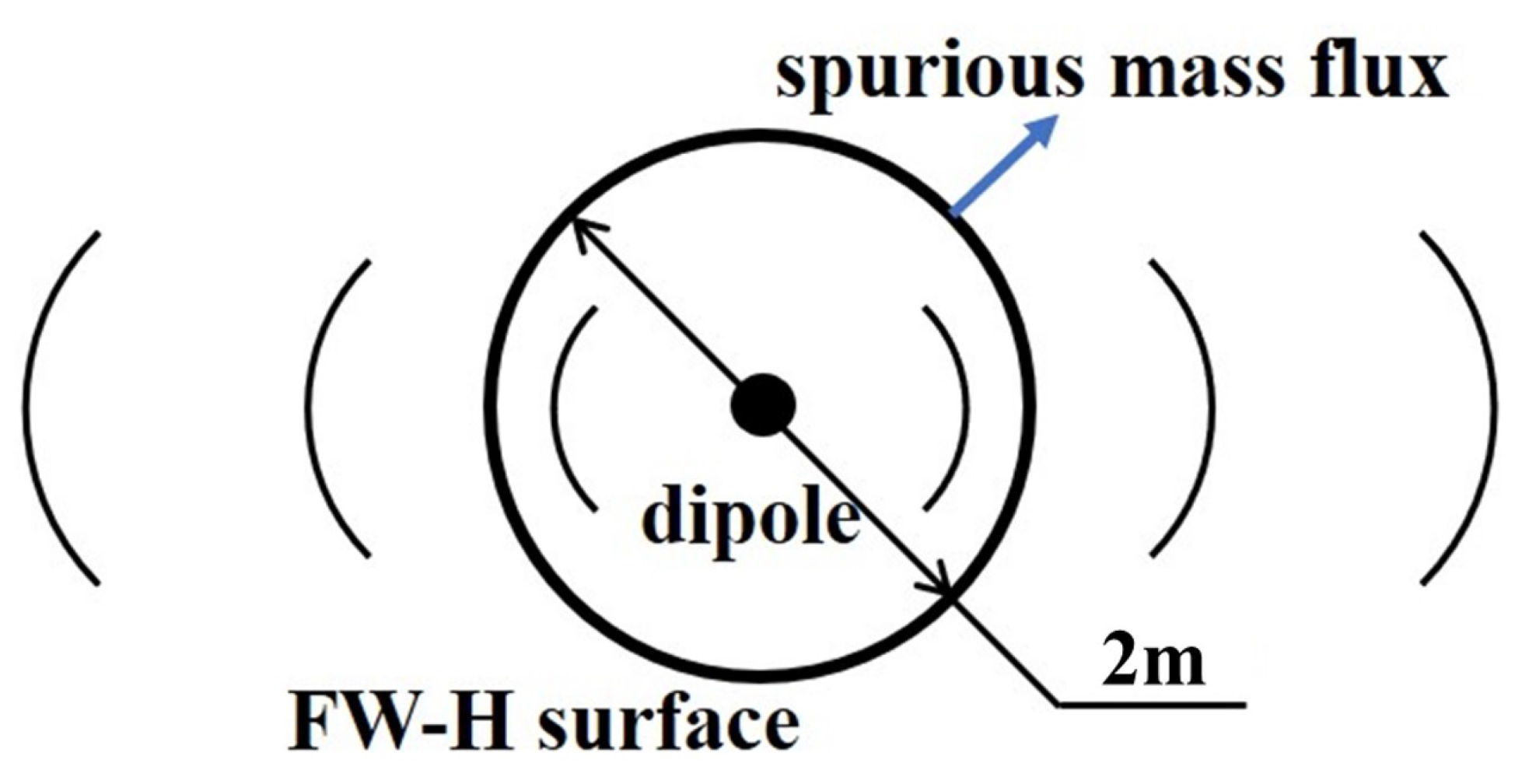
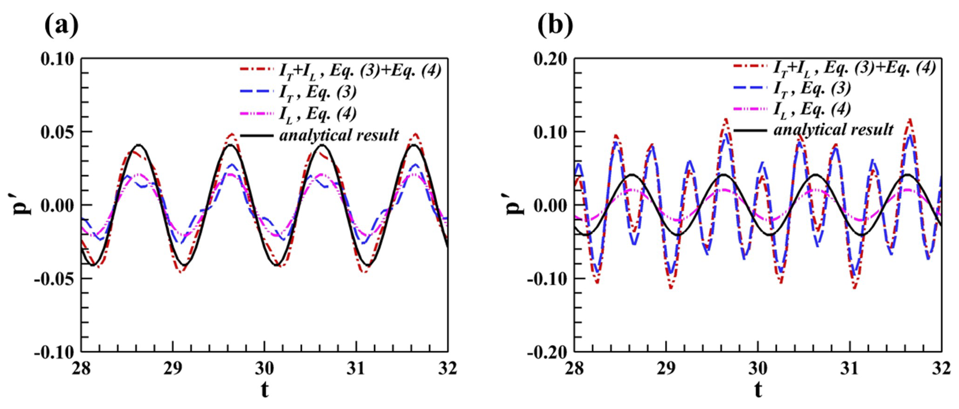
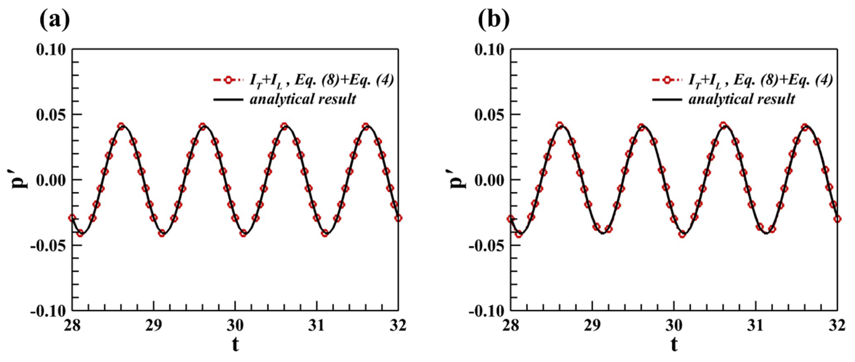
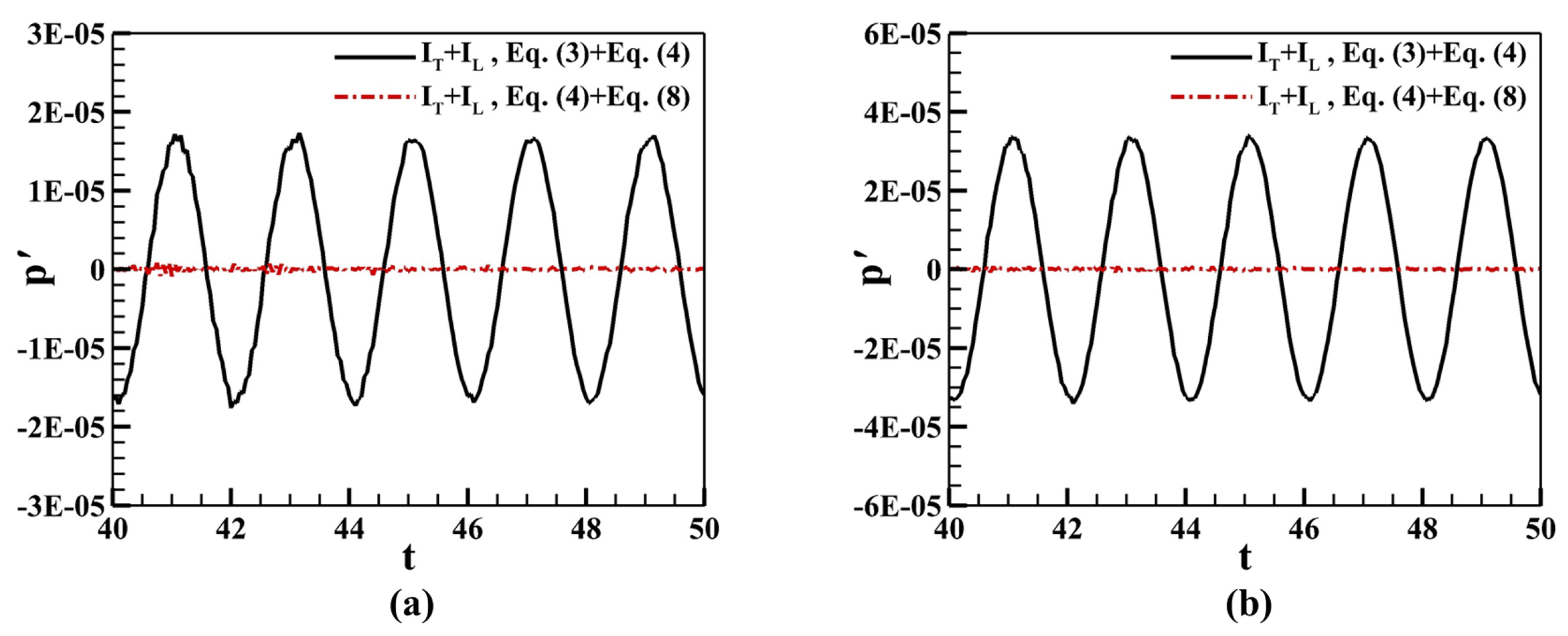
4.1. Unsteady Dipole in a Steady Ambient Flow

The dipole consists of a source and sink separated by a small distance. The potential function of the dipole in steady ambient flow is given by [25]

$$\varphi \left(\mathbf{x},t\right)=\frac{\partial \left(\frac{A\mathrm{i}}{4}{e}^{\mathrm{i}{\omega }_{0}t}{H}_0^{\left(2\right)}\left(\frac{{\omega }_0}{c_0}\sqrt{x_1^2+x_2^2}\right)\right)}{\partial x_1},$$

(16)

where A and ${\omega }_0$ are $0.02{\mathrm{m}}^2/\mathrm{s}$ and $2\pi \mathrm{rad}/\mathrm{s}$, respectively, and $H_0^{\left(2\right)}$ is the zeroth-order Hankel function of the second kind. The perturbations of pressure, density, and velocity are obtained as follows:

$$\begin{array}{cc}\hfill p^{\prime }(\mathbf{y},\omega )=& -\mathrm{i}\omega {\rho }_0\varphi (\mathbf{y},\omega )\hfill \\ \hfill {\rho }^{\prime }(\mathbf{y},\omega )=& \frac{p^{\prime }(\mathbf{y},\omega )}{c_0^2},\hfill \\ \hfill u_i^{\prime }(\mathbf{y},\omega )=& \frac{\partial \varphi (\mathbf{y},\omega )}{\partial y_i},\hfill \end{array}$$

(17)

where ${\rho }_0$ and $c_0$ are $1\mathrm{kg}/{\mathrm{m}}^3$ and $340\mathrm{m}/\mathrm{s}$, respectively. The permeable FW–H boundary is taken as a circle of diameter $2\mathrm{m}$. To discuss the effects of the spurious mass flux on the far-field sound, a spurious mass flux is defined on the FW–H boundary by adding extra velocity ${\mathbf{u}}_e$ (defined below), as shown in Figure 1:

$${\mathbf{u}}_e=A_{e}sin\left({\omega }_{e}t\right)\left(\frac{y_1}{\sqrt{y_1^2+y_2^2}},\frac{y_2}{\sqrt{y_1^2+y_2^2}}\right),$$

(18)

where $A_e$ and ${\omega }_e$ are the amplitude and frequency of the extra velocity, respectively. The spurious mass flux can be derived according to the extra velocity ${\mathbf{u}}_e$ as

$${\stackrel{•}{m}}_s=\pi {\rho }_0{D}_{FWH}{A}_{e}sin\left({\omega }_{e}t\right),$$

(19)

where $D_{FWH}$ is the diameter of the FW–H boundary.

In this section, the frequency ${\omega }_e$, as distinct from the frequency of the unsteady dipole ${\omega }_0$, is taken to be $5\pi \mathrm{rad}/\mathrm{s}$. The amplitude $A_e$ is defined to be $1\times {10}^{-6}\mathrm{m}/\mathrm{s}$ and $1\times {10}^{-5}\mathrm{m}/\mathrm{s}$, corresponding to the maximum instantaneous mass fluxes $1.26\times {10}^{-5}\mathrm{kg}/\mathrm{s}$ and $1.26\times {10}^{-4}\mathrm{kg}/\mathrm{s}$, respectively. Since the mass inside the closed FW–H boundary is $12.56\mathrm{kg}$, the maximum relative spurious mass change per second is 0.0001% or 0.001%, depending on whether the averaged velocity divergence is $1\times {10}^{-6}/\mathrm{s}$ or $1\times {10}^{-5}/\mathrm{s}$, respectively.

Figure 2 shows the acoustic pressure at the observer’s location $\frac{100c_0{\omega }_0}{2\pi }\left(cos\left(\frac{\pi }{4}\right),sin\left(\frac{\pi }{4}\right)\right)$ by using the formulation without filtering the spurious mass flux (Equation (3) + Equation (4)). In Figure 2a, the computed acoustic pressure is represented by the red dash–dot line, while the analytical result is the black solid line. The monopole term and the dipole are the blue dashed line and purple dash–dot–dot line. The fictitious harmonics can be observed in the acoustic pressure $I_T+I_L$ and the monopole term $I_T$, but are absent in the dipole term $I_L$. The results show that the far-field acoustic pressure is clearly affected by the monopole term when $A_e={10}^{-6}\mathrm{m}/\mathrm{s}$, corresponding to a relative error of 17.4%. Further, when $A_e={10}^{-5}\mathrm{m}/\mathrm{s}$, the acoustic pressure is dominated by the monopole term, as shown in Figure 2b, corresponding to a relative error of 186.9%. This suggests that the spurious mass flux will result in a spurious monopole term, thereby leading to a false acoustic pressure even at an average velocity divergence of $1\times {10}^{-6}/\mathrm{s}$.

The far-field acoustic pressure computed by using the mass-conserved monopole term, Equation (8), is shown in Figure 3; the observer position is $\frac{100c_0{\omega }_0}{2\pi }\left(cos\left(\frac{\pi }{4}\right),sin\left(\frac{\pi }{4}\right)\right)$. With the spurious mass flux filtered, the results show good agreement with the analytical solution for both cases. The maximum relative errors reduce to 0.2% and 1.8% at the peak of the acoustic pressure fluctuation.

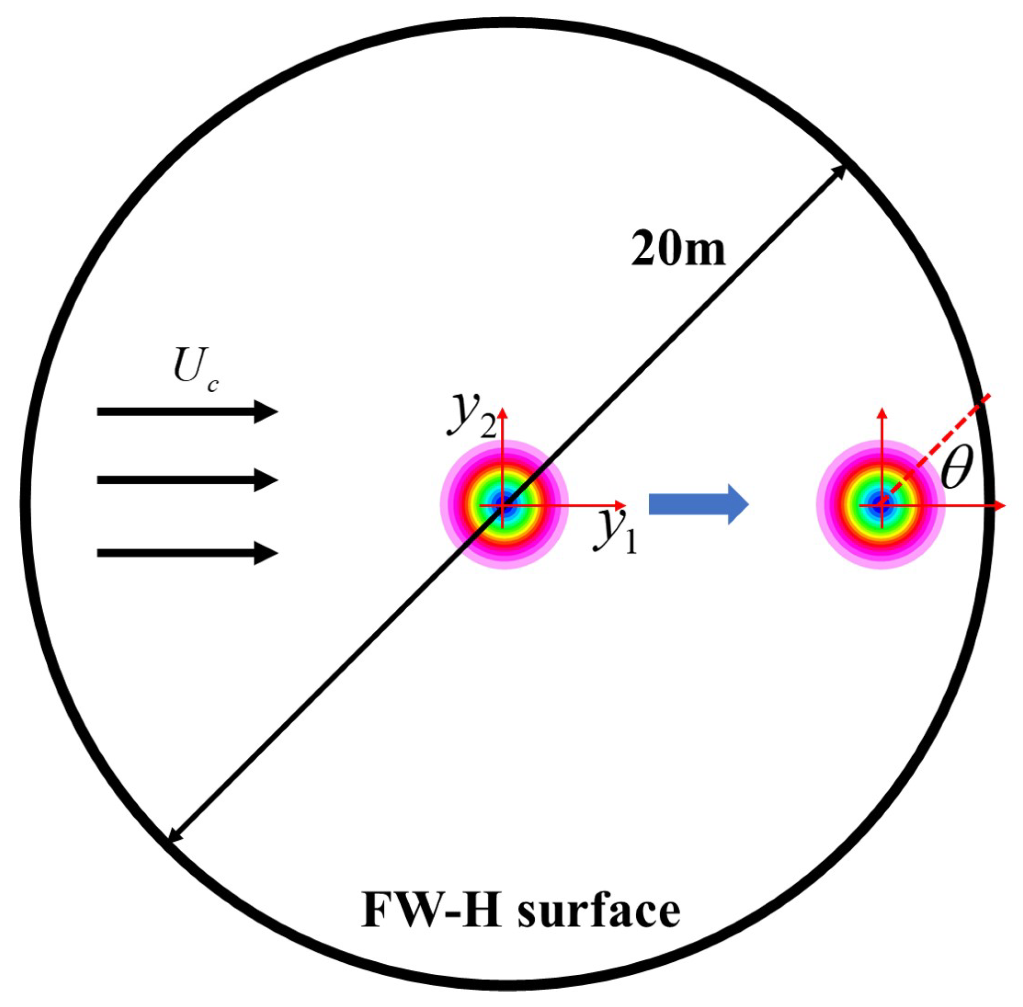
4.2. 2D Incompressible Convecting Vortex

We use the 2D incompressible convecting vortex [13] to validate the proposed mass-conserved formulation. The pressure and velocity field of the 2D incompressible convecting vortex are given by

$$\begin{array}{cc}\hfill u_1(\mathbf{y},\tau )& =U_c+\frac{\mathrm{\Gamma }}{2\pi r}sin\left(\theta \right),\hfill \\ \hfill u_2(\mathbf{y},\tau )& =\frac{-\mathrm{\Gamma }}{2\pi r}cos\left(\theta \right),\hfill \\ \hfill p(\mathbf{y},\tau )& =p_0-\frac{\rho {\mathrm{\Gamma }}^2}{8{\pi }^2{r}^2},\hfill \end{array}$$

(20)

where $U_c$ is the uniform freestream velocity. $\mathrm{\Gamma }$ is the circulation of the vortex. As is shown in Figure 4, r is the distance from the observer to the moving vortex’s center, and $\theta$ represents the angle with respect to the vortex’s center. $p_0$ is the pressure in the ambient flow. The density $\rho$ is assumed to be ${\rho }_0$. We take the uniform freestream velocity $U_c$ to be 0.1 m/s, the speed of sound to be 340 m/s, the circulation of the vortex to be $\mathrm{\Gamma }=1{\mathrm{m}}^2/\mathrm{s}$, the density in the ambient flow to be ${\rho }_0=1\mathrm{kg}/{\mathrm{m}}^3$, and the pressure in the ambient flow to be $p_0=0\mathrm{Pa}$. According to the reference [13], the far-field acoustic pressure approaches ero. Therefore, the convecting vortex is suitable for investigating the effects of spurious mass flux across the FW–H surface. We take the permeable FW–H surface to be a circle of diameter 20 m. The spurious mass flux is given by adding extra velocity ${\mathbf{u}}_{\mathbf{e}}$, which is consistent with the unsteady dipole case, as follows:

$$\begin{array}{c}\hfill {\mathbf{u}}_e=A_{e}sin\left({\omega }_{e}t\right)\left(\frac{y_1}{\sqrt{y_1^2+y_2^2}},\frac{y_2}{\sqrt{y_1^2+y_2^2}}\right).\end{array}$$

(21)

${\omega }_e$ and $A_e$ are the frequency and amplitude of the spurious mass flux. We take the frequency ${\omega }_e$ to be $5\pi \mathrm{rad}/\mathrm{s}$.

We compare the acoustic pressure at the observer location $(30,000\sqrt{2}\mathrm{m},30,000\sqrt{2}\mathrm{m})$ with and without filtering the spurious mass flux, as is shown in Figure 5. The amplitude of the spurious mass flux $A_e$ for the cases shown in Figure 5a,b are $10^{-5}\mathrm{m}/\mathrm{s}$ and $2\times 10^{-5}\mathrm{m}/\mathrm{s}$, respectively. The black solid line represents the result computed by using the formulation without filtering the spurious mass flux (Equation (3) + Equation (4)). The red dash–dot line represents the result computed by filtering the spurious mass flux (Equation (4) + Equation (8)). It is observed that the spurious mass flux leads to an erroneous harmonic signal of the far-field acoustic pressure, as is shown in Figure 5. Meanwhile, the erroneous harmonic signal is significantly suppressed by filtering the spurious mass flux term. This result shows that the far-field acoustic pressure is sensitive to the spurious mass flux with sound sources from incompressible flows, and the mass-conserved formulation is applicable to prediction of sound generated from incompressible flows.

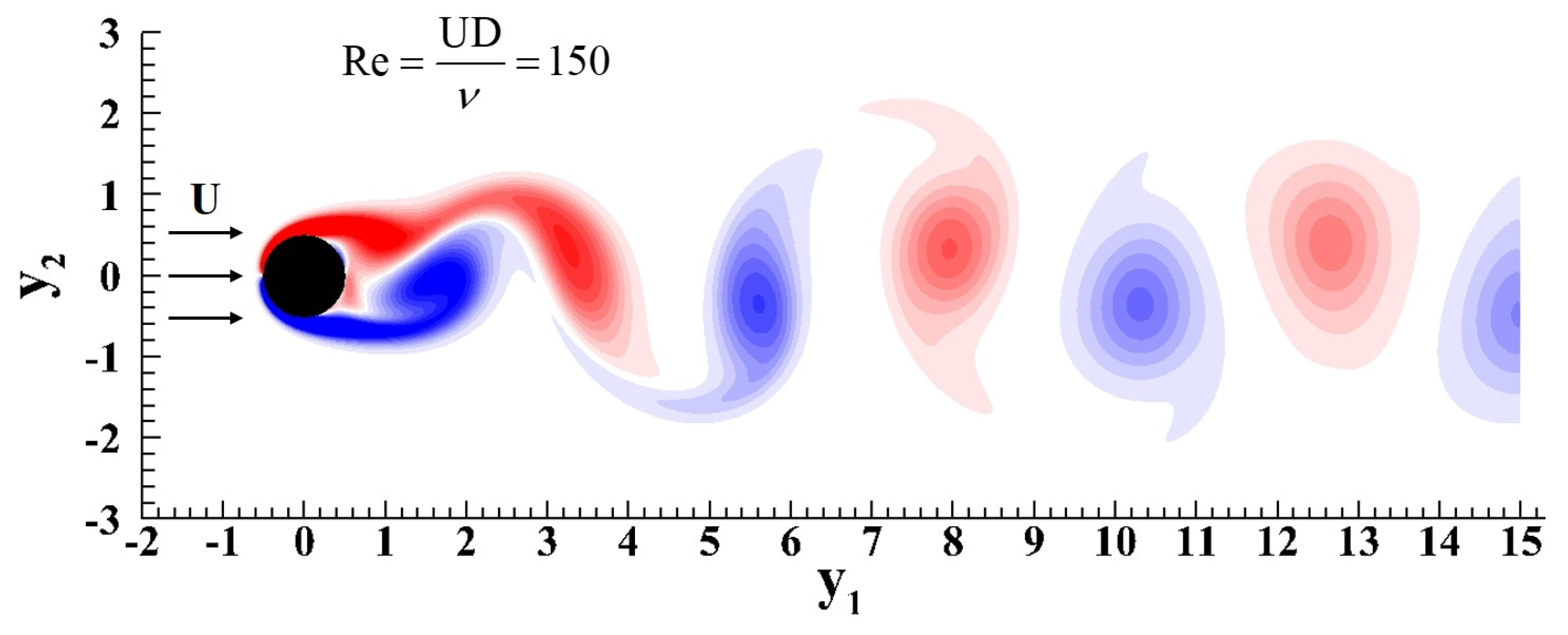
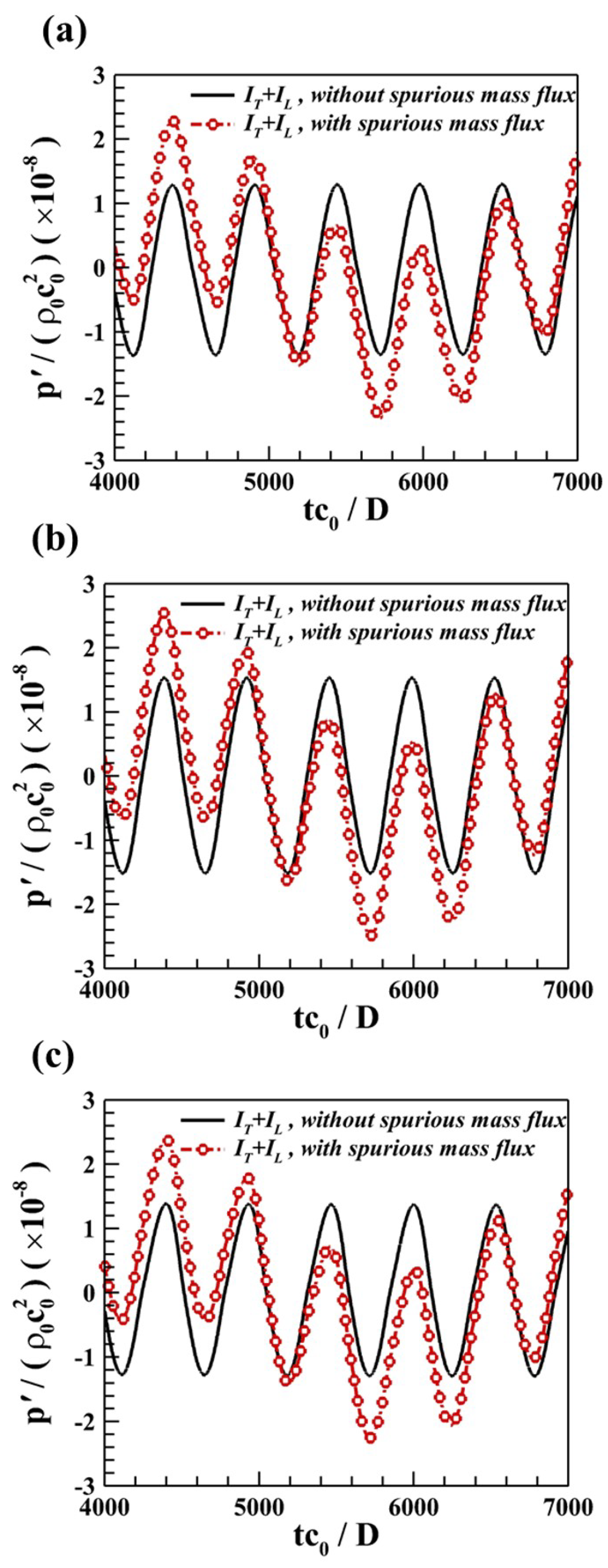
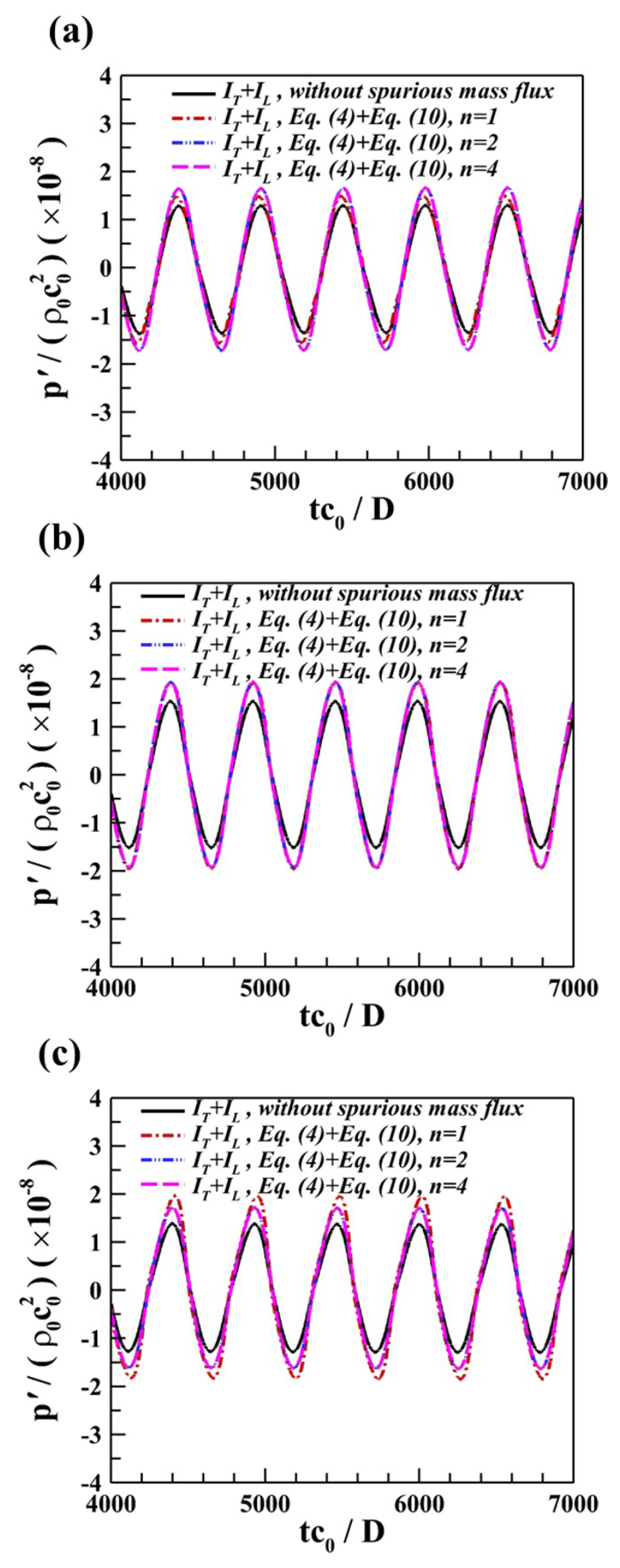
4.3. Flows over a Circular Cylinder

Flows over a circular cylinder at low Reynolds numbers have been widely used to examine different sound prediction methods. In this section, we computed the acoustic pressure radiated by flows over a circular cylinder at a Reynolds number of 150, which was also examined using a direct numerical simulation [26], the FW–H integral [13], and a tailored Green’s function [27]. To validate the proposed formulation, the far-field acoustic pressure was computed by summing the dipole term, Equation (4); and the monopole terms, Equations (3) and (10), with a permeable integral boundary, including spurious mass flux. The results are compared with the computed acoustic pressure without adding spurious mass flux. The results, with different numbers of expansion points in Equation (10) are discussed to show the dominant term of the monopole equation at very low Mach numbers.

The flows over a circular cylinder were simulated by using an in-house CFD solver, where the Naver–Stokes equations for incompressible flows were discretized with a second-order finite difference method. We have revised the manuscript by declaring the CFD solver and the related paper [28]. The circular cylinder of diameter D, centered at the origin, is shown in Figure 6. The freestream speed was U, the Reynolds number based on D and U was 150, and the streamwise and vertical directions correspond to the $y_1$ and $y_2$ axes, respectively. In the simulation of flows over a circular cylinder, the Navier–Stokes equations for incompressible flows are solved in the near field to obtain the sources of sound. Therefore, the uniform flow is specified at the inlet. The free convection boundary condition is applied at the outlet. The other two sides are slip walls. The immersed boundary method is employed to implement the no-slip wall condition on the circular-cylinder’s surface. The computation domain ranges from −10 to $15D$ and −12 to $12D$ along the $y_1$ and $y_2$ axes, respectively. The mesh size was set as 0.01D, and the time step was taken as $0.01D$ or $0.001D/U$ according to the work of Wang et al. [28]. The time step and mesh size are sufficiently small to provide reasonable pressure and velocity fields. The detailed numerical resolution can be found in the work of Wang et al. [28].

When the integral boundary is taken to be permeable, the monopole term, as Equation (3), needs to be computed, and the spurious mass flux may result in significant error. To examine the contribution from the spurious mass flux, a closed rectangular integral boundary was taken from the source region. The upstream and downstream integral boundaries are $y_1=-D$ and $y_1=4D$, respectively. The other two integral boundaries are $y_2=\pm D$. The sampling step for far-field sound computation was $0.027D/U$. The speed of sound is $100U$, which leads to a characteristic sound wavelength of $100D$. The source region is thus compact and nearly incompressible. The observer was chosen to be $1000D$ away from the origin, ensuring the far-field condition.

A spurious mass flux was defined by using Equation (16) on the integral boundary. The frequency ${\omega }_e$ was taken to be $2.5\pi U/D$. The amplitude $A_e$ was defined to be $2\times {10}^{-4}U$, corresponding to the maximum instantaneous mass flux $4\times {10}^{-3}{\rho }_{0}UD$. Since the mass inside the closed FW–H boundary is $40{\rho }_0{D}^2$, the maximum relative spurious mass change in unit time is 0.02%, related to an averaged velocity divergence of $2\times {10}^{-4}U/D$. Such a velocity divergence may appear in the turbulence simulation with a non-conservative scheme.

Figure 7 shows the acoustic pressure, computed by summing the monopole and dipole terms, Equations (3) and (4), at the observer locations $1000D\left(cos\left(\frac{\pi }{3}\right),sin\left(\frac{\pi }{3}\right)\right)$, $1000D\left(cos\left(\frac{\pi }{2}\right),sin\left(\frac{\pi }{2}\right)\right)$, and $1000D\left(cos\left(\frac{2\pi }{3}\right),sin\left(\frac{2\pi }{3}\right)\right)$, respectively. The red dash–dot line is a result of the acoustic pressure with spurious mass flux. The result without the spurious mass flux is plotted with the black solid line. Significant errors in acoustic pressure prediction are present owing to the spurious mass flux. The maximum relative errors of the acoustic pressure at the ${60}^{\circ },{90}^{\circ },$ and ${120}^{\circ }$ observer points are 78.1%, 65.4%, and 71.9%, respectively. The observer point at the ${90}^{\circ }$ direction is least affected by the spurious mass flux. This is probably because the dipole term at ${90}^{\circ }$ makes a greater contribution to the acoustic pressure than at other angles.

Figure 8 shows the acoustic pressure computed by summing the dipole term Equation (4) and the expansion of the mass-conserved monopole term Equation (10) for $n=1,2$, and 4. By using the mass-conserved formulation, Equation (10), the fictitious harmonics are clearly filtered. The maximum amplitude errors reduce from 78.1%, 65.4%, and 71.9% to 28.4%, 26.0%, and 25.6% at the observer locations of 60°, 90°, and 120°, respectively. The mass-conserved formulation (Equation (4) + Equation (10)) converges when $n=1$ at the observer location of 90°. At the 60° and 120° points, the mass-conserved formulation converges when $n=2$, and the first-order term still dominates the monopole term. The results show that the expansion of the mass-conserved formulation can reduce the effects of spurious mass flux with little extra cost. In addition, the results imply that the monopole term is nearly dominated by the momentum flux, namely, the first-order term in Equation (10), at very low Mach numbers. Further, Equations (10) and (13) suggest that the first-order term gives directivity to the dipole. It is quite different from sound generated by high-lift wings at the freestream Mach number 0.2, where the mass flux is supposed to dominate the monopole term and the far-field acoustic pressure [29].

4.4. Co-Rotating Vortex Pair

The co-rotating vortex pair is a classic simplified model for investigating jet noise generated by coherent structures. The mechanism of vortex-pair sound radiation has been clarified by Feng et al. [30] using spectral-acoustic analogy theory based on the direct numerical simulation of two compressible Gaussian vortices: combinations of two co-rotating vortices, including four stages, which can be observed by the far-field acoustic pressure. Thus, by simulating a co-rotating vortex pair, a non-periodic source field can be obtained. In this part, we applied the mass-conserved monopole term, Equation (10), to the far-field sound prediction without adding extra spurious mass flux. The sensitivity of the far-field acoustic pressure to the integral boundary position is also discussed.

We numerically solved the incompressible Navier–Stokes equation using the Nek5000 solver, to obtain the source field. According to the work of Mao et al. [31], the initial flow field consists of two Guassian vortices, as in Figure 9.

${\mathrm{\Gamma }}_0$ and $U_0$ are the circulation and rotating velocity of each vortex. $D_0$ and $r_0$ are the initial distance between vorticities and the radius of a vortex. The tangential velocity distribution of a Guassian vortex is given by

$$u_{\theta }=\frac{{\mathrm{\Gamma }}_0}{2\pi r}\left(1-e^{-\frac{r^2}{r_0^2}}\right),$$

(22)

where r is the distance between the source position and the vortex’s center. In this case, we take ${\mathrm{\Gamma }}_0$ and $D_0$ as the non-dimensionalized basis, $r_0=0.25D_0$, and the Reynolds number based on ${\mathrm{\Gamma }}_0$ as 10,000. The streamwise and vertical directions correspond to $y_1$ and $y_2$ axes, respectively, and the computational domain ranges from $-5\pi D_0$ to $5\pi D_0$ and $-5\pi D_0$ to $5\pi D_0$ along the $y_1$ and $y_2$ axes, respectively.

Figure 10 shows the far-field acoustic pressure computed by summing the monopole and dipole terms, Equations (3) and (4), without filtering the spurious mass flux. The speed of sound is $18{\mathrm{\Gamma }}_0/D_0$, and the observer’s location is at $1250D_0\left(cos\frac{\pi }{4},sin\frac{\pi }{4}\right)$. We sampled the source region over $25D_{{}_0}^2/18{\mathrm{\Gamma }}_0$ with 1000 time steps. The solid black line, long red dashed line, blue dash–dot line, and purple dash–dot–dot line correspond to the integral boundaries of $[-\frac{5}{3}{D}_0,\frac{5}{3}{D}_0]\times [-\frac{5}{3}{D}_0,\frac{5}{3}{D}_0]$, $[-2.5D_0,2.5D_0]\times [-2.5D_0,2.5D_0]$, $[-\frac{10}{3}{D}_0,\frac{10}{3}{D}_0]\times [-\frac{10}{3}{D}_0,\frac{10}{3}{D}_0]$, and $[-\frac{25}{6}{D}_0,\frac{25}{6}{D}_0]\times [-\frac{25}{6}{D}_0,\frac{25}{6}{D}_0]$, which are represented by the side lengths in Figure 10, respectively. It is observed that the far-field acoustic pressure converges with the extension of the integral boundary. However, the acoustic pressure from 12.5 $D_{{}_0}^2/{\mathrm{\Gamma }}_0$ to 25 $D_{{}_0}^2/{\mathrm{\Gamma }}_0$ presents an obvious inconsistency related to the integral boundary of $[-\frac{5}{3}{D}_0,\frac{5}{3}{D}_0]\times [-\frac{5}{3}{D}_0,\frac{5}{3}{D}_0]$, whereas during the rest time, there remains consistency. This may result from the non-negligible residual of the continuity equation. To validate this, we employed the mass-conserved formulation (Equation (4) + Equation (8)) to compute the far-field acoustic pressure. The results are plotted in Figure 11. It is shown that the inconsistency during [12.5 $D_{{}_0}^2/{\mathrm{\Gamma }}_0$,25 $D_{{}_0}^2/{\mathrm{\Gamma }}_0$] is eliminated by filtering the spurious mass flux. This implies that the integral boundary position dependence of far-field sound prediction may result from the spurious mass flux, and our proposed mass-conserved formulation is able to suppress the dependence by filtering the spurious mass flux.

5. Conclusions

The spurious mass flux was found to significantly affect the prediction of far-field sound within the FW–H acoustic analogy. To filter the contribution from the spurious mass flux, we have proposed a mass-conserved formulation of the monopole term in the frequency-domain solution to the FW–H equation. The formulation is especially suitable for predicting far-field acoustic pressure at very low Mach numbers with a static permeable FW–H boundary. The contribution to the far-field acoustic pressure from the spurious mass flux through the integral boundary is significantly suppressed by using the proposed formulation. The compact-source region assumption is employed to calculate the contribution from the spurious mass flux to the far-field acoustic pressure. The asymptotic Green’s function’s higher-order derivatives are used to expand the monopole term after eliminating the mass-flux-dominated term. From the expansion, we observe that the first term can be simplified to a scaled momentum fluctuation of the fluid inside the integral boundary.

The proposed mass-conserved formulation was validated by using an unsteady dipole, a 2D incompressible convecting vortex, flows over a circular cylinder, and a co-rotating vortex pair. The results of the dipole case show that a relative spurious mass flux of 0.001% per unit time may result in a significant error of up to 186.9% in the far-field acoustic pressure with direct use of FW–H surface integrals. By using the mass-conserved monopole term, the relative error reduces to 1.8%. The expansion of the mass-conserved monopole term was discussed with the circular-cylinder flow. By using the expansions of order $n=1,2,$ and 4, we found that the predicted acoustic pressure converges quickly, and the expansion is dominated by the first term. Further simplifications show that the first order of the expansion is the product of the total momentum fluctuation in the integral boundary and a coefficient showing dipole directivity. This result suggests that at very low Mach numbers, the monopole term may present a directivity of a dipole owing to the incompressible condition. Finally, an incompressible-flow simulation of a co-rotating vortex pair was performed without adding spurious mass flux. An inconsistency of the predicted far-field sound was observed with different sizes of the permeable FW–H boundary. By using the mass-conserved monopole term, the integral boundary dependence is circumvented. In addition, although the cases mentioned above are all 2D, the 3D mass-conserved formulation for the monopole term was still provided (using substitution in Green’s function).

References

1. Keller, J.; Kumar, P.; Mahesh, K. Examination of propeller sound production using large eddy simulation. Phys. Rev. Fluids 2018, 3, 064601. [Google Scholar] [CrossRef]
2. Lidtke, A.K.; Turnock, S.R.; Humphrey, V.F. Characterisation of sheet cavity noise of a hydrofoil using the Ffowcs Williams–Hawkings acoustic analogy. Comput. Fluids 2016, 130, 8–23. [Google Scholar] [CrossRef]
3. Zhou, Z.T.; Xu, Z.Y.; Wang, S.Z.; He, G.W. Wall-modeled large-eddy simulation of noise generated by turbulence around an appended axisymmetric body of revolution. J. Hydrodyn. 2022, 34, 533–554. [Google Scholar] [CrossRef]
4. Wang, X.; Huang, Q.; Pan, G. Numerical research on the influence of sail leading edge shapes on the hydrodynamic noise of a submarine. Appl. Ocean. Res. 2021, 117, 102935. [Google Scholar] [CrossRef]
5. Powell, A. Theory of vortex sound. J. Acoust. Soc. Am. 1964, 36, 177–195. [Google Scholar] [CrossRef]
6. Möhring, W. On vortex sound at low Mach number. J. Fluid Mech. 1978, 85, 685–691. [Google Scholar] [CrossRef]
7. Schram, C.; Hirschberg, A. Application of vortex sound theory to vortex-pairing noise: Sensitivity to errors in flow data. J. Sound Vib. 2003, 266, 1079–1098. [Google Scholar] [CrossRef]
8. Williams, J.F.; Hawkings, D.L. Sound generation by turbulence and surfaces in arbitrary motion. Philos. Trans. R. Soc. Lond. Ser. A Math. Phys. Sci. 1969, 264, 321–342. [Google Scholar]
9. Cianferra, M.; Ianniello, S.; Armenio, V. Assessment of methodologies for the solution of the Ffowcs Williams and Hawkings equation using LES of incompressible single-phase flow around a finite-size square cylinder. J. Sound Vib. 2019, 453, 1–24. [Google Scholar] [CrossRef]
10. Wang, M.; Lele, S.K.; Moin, P. Computation of quadrupole noise using acoustic analogy. AIAA J. 1996, 34, 2247–2254. [Google Scholar] [CrossRef]
11. Zhou, Z.; Wang, H.; Wang, S.; He, G. Lighthill stress flux model for Ffowcs Williams–Hawkings integrals in frequency domain. AIAA J. 2021, 59, 4809–4814. [Google Scholar] [CrossRef]
12. Lockard, D.; Casper, J. Permeable surface corrections for Ffowcs Williams and Hawkings integrals. In Proceedings of the 11th AIAA/CEAS Aeroacoustics Conference, Monterey, CA, USA, 23–25 May 2005; p. 2995. [Google Scholar]
13. Nitzkorski, Z.; Mahesh, K. A dynamic end cap technique for sound computation using the Ffowcs Williams and Hawkings equations. Phys. Fluids 2014, 26, 115101. [Google Scholar] [CrossRef]
14. Testa, C.; Porcacchia, F.; Zaghi, S.; Gennaretti, M. Study of a FWH-based permeable-surface formulation for propeller hydroacoustics. Ocean. Eng. 2021, 240, 109828. [Google Scholar] [CrossRef]
15. Zhong, S.; Zhang, X. A sound extrapolation method for aeroacoustics far-field prediction in presence of vortical waves. J. Fluid Mech. 2017, 820, 424–450. [Google Scholar] [CrossRef]
16. Zhong, S.; Zhang, X. A generalized sound extrapolation method for turbulent flows. Proc. R. Soc. A Math. Phys. Eng. Sci. 2018, 474, 20170614. [Google Scholar] [CrossRef]
17. Yao, H.D.; Davidson, L.; Eriksson, L.E. Noise radiated by low-Reynolds number flows past a hemisphere at Ma= 0.3. Phys. Fluids 2017, 29, 076102. [Google Scholar] [CrossRef]
18. Ricciardi, T.R.; Wolf, W.R.; Spalart, P.R. On the Application of Incomplete Ffowcs Williams and Hawkings Surfaces for Aeroacoustic Predictions. AIAA J. 2022, 60, 1971–1977. [Google Scholar] [CrossRef]
19. Shur, M.L.; Spalart, P.R.; Strelets, M.K. Noise prediction for increasingly complex jets. Part I: Methods and tests. Int. J. Aeroacoustics 2005, 4, 213–245. [Google Scholar] [CrossRef]
20. Zhou, Z.; Zang, Z.; Wang, H.; Wang, S. Far-field approximations to the derivatives of Green’s function for the Ffowcs Williams and Hawkings equation. Adv. Aerodyn. 2022, 4, 12. [Google Scholar] [CrossRef]
21. Zhou, Z.; Wang, H.; Wang, S.; He, G. Quadrupole source term corrections based on correlation functions for Ffowcs Williams and Hawkings integrals. Acta Aerodyn. Sin. 2020, 38, 1129–1135. [Google Scholar]
22. Brentner, K.S.; Farassat, F. Modeling aerodynamically generated sound of helicopter rotors. Prog. Aerosp. Sci. 2003, 39, 83–120. [Google Scholar] [CrossRef]
23. Lockard, D.P. An efficient, two-dimensional implementation of the Ffowcs Williams and Hawkings equation. J. Sound Vib. 2000, 229, 897–911. [Google Scholar] [CrossRef]
24. Zhou, Z.; Wang, H.; Wang, S. Simplified permeable surface correction for frequency-domain Ffowcs Williams and Hawkings integrals. Theor. Appl. Mech. Lett. 2021, 11, 100259. [Google Scholar] [CrossRef]
25. Najafi-Yazdi, A.; Brès, G.A.; Mongeau, L. An acoustic analogy formulation for moving sources in uniformly moving media. Proc. R. Soc. A Math. Phys. Eng. Sci. 2011, 467, 144–165. [Google Scholar] [CrossRef]
26. Inoue, O.; Hatakeyama, N. Sound generation by a two-dimensional circular cylinder in a uniform flow. J. Fluid Mech. 2002, 471, 285–314. [Google Scholar] [CrossRef]
27. Gloerfelt, X.; Pérot, F.; Bailly, C.; Juvé, D. Flow-induced cylinder noise formulated as a diffraction problem for low Mach numbers. J. Sound Vib. 2005, 287, 129–151. [Google Scholar] [CrossRef]
28. Wang, S.; Vanella, M.; Balaras, E. A hydrodynamic stress model for simulating turbulence/particle interactions with immersed boundary methods. J. Comput. Phys. 2019, 382, 240–263. [Google Scholar] [CrossRef]
29. Yao, H.D.; Davidson, L.; Eriksson, L.E.; Peng, S.H.; Grundestam, O.; Eliasson, P.E. Surface integral analogy approaches for predicting noise from 3D high-lift low-noise wings. Acta Mech. Sin. 2014, 30, 326–338. [Google Scholar] [CrossRef]
30. Feng, F.; Meng, X.; Wang, Q. Sound generation by a pair of co-rotating vortices using spectral acoustic analogy. J. Sound Vib. 2020, 469, 115120. [Google Scholar] [CrossRef]
31. Mao, F.; Kang, L.; Wu, J.; Yu, J.L.; Gao, A.; Su, W.; Lu, X.Y. A study of longitudinal processes and interactions in compressible viscous flows. J. Fluid Mech. 2020, 893. [Google Scholar] [CrossRef]
Figure 1. Schematic of the unsteady dipole source with spurious mass flux on the FW–H boundary.
Aerospace 10 00148 g001
Figure 2. Acoustic pressure calculated by summing Equations (3) and (4) with spurious mass flux on the integral boundary corresponding to (a) A e = 10 6 m / s and (b) A e = 10 5 m / s .
Aerospace 10 00148 g002
Figure 3. Acoustic pressure calculated by summing Equations (8) and (4) with spurious mass flux on the integral boundary corresponding to (a) A e = 10 6 m / s and (b) A e = 10 5 m / s .
Aerospace 10 00148 g003
Figure 4. Schematic of the incompressible convecting vortex.
Aerospace 10 00148 g004
Figure 5. Comparison between the acoustic pressure with filtering the spurious mass flux (Equation (4) + Equation (8)) and without filtering the spurious mass flux (Equation (3) + Equation (4)) on the integral boundary corresponding to (a) A e = 10 5 m / s and (b) A e = 2 × 1 0 5 m / s .
Aerospace 10 00148 g005
Figure 6. Schematic of the flows over a circular cylinder at a Reynolds number of 150.
Aerospace 10 00148 g006
Figure 7. Acoustic pressure calculated by summing Equations (3) and (4) with spurious mass flux on the integral boundary at the observer: (a) 1000 D cos π 3 , sin π 3 , (b) 1000 D cos π 2 , sin π 2 , (c) 1000 D cos 2 π 3 , sin 2 π 3 .
Aerospace 10 00148 g007
Figure 8. Acoustic pressure calculated by summing Equations (4) and (10) for n = 1 , 2 , 4 with spurious mass flux on the integral boundary at the observer: (a) 1000 D cos π 3 , sin π 3 , (b) 1000 D cos π 2 , sin π 2 , (c) 1000 D cos 2 π 3 , sin 2 π 3 , respectively.
Aerospace 10 00148 g008
Figure 9. Schematic of the co-rotating vortex pair.
Aerospace 10 00148 g009
Figure 10. Acoustic pressure calculated by summing Equations (3) and (4) without filtering the spurious mass flux at the observer 1250 D 0 cos π 4 , sin π 4 .
Aerospace 10 00148 g010
Figure 11. Acoustic pressure calculated by summing Equations (8) and (4) when filtering the spurious mass flux at the observer 1250 D 0 cos π 4 , sin π 4 .
Aerospace 10 00148 g011
Disclaimer/Publisher’s Note: The statements, opinions and data contained in all publications are solely those of the individual author(s) and contributor(s) and not of MDPI and/or the editor(s). MDPI and/or the editor(s) disclaim responsibility for any injury to people or property resulting from any ideas, methods, instructions or products referred to in the content.