Article

Numerical Simulation of Supersonic Turbulent Separated Flows Based on k–ω Turbulence Models with Different Compressibility Corrections

School of Energy and Power Engineering, University of Shanghai for Science and Technology, Shanghai 200093, China
Aerospace 2023, 10(12), 1014; https://doi.org/10.3390/aerospace10121014
Submission received: 7 October 2023 / Revised: 15 November 2023 / Accepted: 29 November 2023 / Published: 4 December 2023
(This article belongs to the Special Issue High Speed Flows: Measurements & Simulations)

Abstract

:
The accurate prediction of supersonic turbulent separated flows involved in aerospace vehicles is a great challenge for current numerical simulations. Based on the k–ω equations, several different compressibility corrections are incorporated in turbulence models to improve their prediction capabilities. Two benchmark test cases, namely the ramped cavity and the compression corner, are adopted for the numerical validation. Detailed comparisons between simulations and experiments are conducted to evaluate the effect of compressibility corrections on turbulence models. The computed results indicate that compressibility corrections have a significant impact on turbulence model performance. The compressibility correction, considering the effects of both dilatation dissipation and pressure dilatation, is suitable for the prediction of compressible free shear layers, but it may have a negative impact on the prediction of low-speed flows in the near-wall region due to the severe underprediction of the wall skin friction coefficient. In comparison, the compressibility correction only considering the effects of dilatation dissipation is conservative, with decreased predictability of free shear layers in supersonic flows, although it improves the predictions of the original models without corrections.

1. Introduction

Supersonic turbulent separation commonly exists in flows around flight vehicles and also in internal combustors. The accurate prediction of turbulent separated flows and a clear understanding of flow physics are important for the better design of flight vehicles. Computational fluid dynamics (CFD) has become an invaluable tool in the design and development of aerospace vehicles. Due to the limitation of computing resources, direct numerical simulations (DNSs) or large eddy simulations (LESs) of supersonic turbulent flows are currently unrealistic in practical engineering applications [1,2]. In the foreseeable future, turbulence models based on statistical theory will still be widely used in the aerodynamic design of vehicles.
Traditionally, turbulence models derived from low-speed incompressible conditions have been directly applied to simulations of compressible turbulence. For high-Mach-number turbulent flows, this approach is highly questionable. As the Mach number increases, the flow compressibility increases, and density fluctuations will have an important effect on the structure of a compressible turbulent flow. Although it is difficult to determine which flow variables cause these changes in flow structure, the role of some new correlation terms that appear in the model after Favre mass-averaging is something that should be considered. A turbulence model that ignores the turbulence Mach number, MT, will have difficulty in accurately estimating the effects of compressibility and thus is not suitable for simulations of supersonic and hypersonic turbulent flows. Sarkar [3] and Zeman [4] have devised very elegant models of compressibility corrections for the simulation of compressible mixing layers. Their work is very innovative and useful, although their models work best only for strained homogeneous flows. Based on previous work, Wilcox [5,6] postulated a similar model, and it shows encouraging applicability to the simulation of wall-bounded flows. Suzen and Hoffmann [7] made compressibility corrections for Menter’s turbulence model and obtained improved predictions for supersonic jet exhaust flows. It should be noted that a certain compressibility correction method that has been proposed has been proven to be effective for a certain class of flows, but its universality for complex compressible flows still needs further verification and confirmation.
As for the research object in the present study, both a ramped cavity and a compression corner are selected as test cases, which are simplified geometric shapes for supersonic turbulent flows with separation. Available experimental data on the two cases are abundant, and a number of CFD calculations have been conducted. Unsteady Reynolds-averaged Navier–Stokes (URANS) calculations (see Horstman et al. [8]) for supersonic ramped cavity flows have been performed and have obtained the overall features of this complex flow field. However, the URANS predictions show large deviations from the experiment. Hybrid RANS/LES computations (see Fan et al. [9], Luo et al. [10], and Yan et al. [11]) have also been conducted, and overall, the results agree well with the experiment. Though consuming considerable computational resources, the capture of three-dimensional transient vortices does improve the URANS results. However, for engineering applications, steady RANS calculations are often preferred due to their shorter computation time and simpler post-processing of flow field data. Moreover, more often than not, time-averaged flow quantities are of more interest. Therefore, suitable RANS methods are required in order to accurately simulate such complex flows at a relatively small computational cost. As for a supersonic flow over a compression corner, which is a benchmark test case for shock/boundary layer interactions (SBLIs), direct numerical simulations (see Tong et al. [12] and Li et al. [13]) have been performed to study the interactions of shock waves with the turbulent boundary layer. DNS investigations are concerned with a relatively small Reynolds number, using nearly 50 million grid points, and the computational results are in good agreement with experiments. On the other hand, LES (see Rizzetta et al. [14]) investigations have been carried out, using more than 5 million grid points, but show significant differences from experimental results, mainly due to the fact that the Reynolds number in the simulation is two orders of magnitude lower than that in the experiments. RANS (see Forsythe et al. [15] and Sinha et al. [16]) investigations have also been performed, and the numerical results have shown that it is a challenge for RANS models without corrections to accurately predict the extent of a separation region at a large corner angle.
Previous studies on compressibility corrections to turbulence models have often focused on a particular class of flows, such as compression corner flows, jet flows, base flows, boundary-layer flows, and so on. It is confusing that a certain correction is effective for one type of flow but not for another type, and the conclusions based on one type of flow are not universally applicable. Based on previous research results, this paper presents numerical simulations for the two selected cases, which represent two very different types of flows, based on the k–ω two-equation turbulence model with different compressibility corrections. Detailed CFD calculations have been conducted and compared to the available experimental data in order to evaluate the effect of compressibility corrections on turbulence models in the simulation of supersonic turbulent separated flows. The purpose of this paper is not to propose a new compressibility correction method but to evaluate the existing methods through typical test cases and to give research suggestions for inspiration.
The paper is organized as follows. In Section 2, numerical methods, including different versions of the k–ω turbulence model and different compressibility correction methods, are introduced. Numerical validation and computational results from different RANS models with or without corrections are presented in Section 3. Conclusions are drawn in Section 4.

2. Numerical Methods

An in-house CFD code is used in the present computations. Based on a structured grid, this code uses a cell-centered finite volume method. It has been designed for the simulation of steady-state or unsteady turbulent flows. The code has been validated for supersonic flows using turbulence models [10]. The Euler fluxes are discretized by Roe’s upwind biased scheme with a MUSCL extrapolation in a cell-centered finite volume formulation. Two-dimensional RANS simulations are performed based on the following three versions of the k–ω turbulence model, namely, the original, baseline (BSL), and shear stress transport (SST) k–ω models. For all simulations, the RANS solution is considered convergent after the L2 norm of the residual of all the variables (mean flow and turbulence equation) drops by nine orders of magnitude.
The original k–ω two-equation turbulence model equation is written as follows [17]:
( ρ k ) t + ( ρ U i k ) x i = P ˜ k β * ρ k ω + x i ( μ + σ k μ t ) k x i ( ρ ω ) t + ( ρ U i ω ) x i = α ν t P ˜ k β ρ ω 2 + x i ( μ + σ ω μ t ) ω x i   P ˜ k = min ( P k ,   10 β * ρ k ω ) ,   P k = μ t S ¯ 2 2 3 ρ k U k x k S ¯ 2 = S 2 2 3 U k x k 2 ,   S 2 = 2 S i j S i j = U i x j + U j x i U i x j
where ρ is the fluid density, k is the turbulent kinetic energy, ω is the specific dissipation rate, S is the strain rate, and Ui, Uj, and Uk are the flow velocities. As for the BSL turbulence model [18,19], the k-equation is formally identical to the original k–ω model. The difference is that a cross-diffusion term is added in the ω-equation, and it is written as [18,19]
( ρ ω ) t + ( ρ U i ω ) x i = γ ν t P ˜ k β ρ ω 2 + x i ( μ + σ ω μ t ) ω x i + 2 ρ ( 1 F 1 ) σ ω 2 ω k x i ω x i
where F1 is the blending function designed by Menter, and its specific expression is given by [18,19]
F 1 = tanh min max k β * ω d ,   500 μ d 2 ρ ω ,   4 ρ σ ω 2 k C D k ω d 2 4 C D k ω = max 2 ρ σ ω 2 ω k x i ω x i ,   10 10
where μ is the fluid dynamic viscosity and d is the distance to the nearest wall. For the calculation of turbulent boundary layers, the performance of the BSL model is very close to that of the original k–ω model, and the turbulent viscosity of both is given by [18,19]
μ t = ρ ν t = ρ k ω
The transport equation of the SST model [18,19] is based on Bradshaw’s assumption that the shear stress, τ, in the boundary layer is proportional to k, which can be expressed as τ = ρa1k, with a1 being a model constant. In the SST model, the transport equations of k and ω are exactly the same as for the BSL model, and the eddy viscosity, μt, is determined by the following equation [18,19]
μ t = min ρ k ω ,   ρ a 1 k S F 2
where F2 is another blending function, and its specific expression is given by [18,19]
F 2 = tanh max 2 k β * ω d ,   500 μ d 2 ρ ω 2
The blending functions F1 and F2 are equal to one inside the boundary layer and switch over to zero away from the wall surface. The model constants for the above three different versions of the k–ω model can be found in the literature [17,18,19].
As for the boundary conditions in turbulence models, the following choice of nondimensional freestream values is adopted:
k a 2 = 9 × 10 9 ,   ω μ ρ a 2 = 1 × 10 6
where a is the free-stream speed of sound. From the above equation, it follows that the free-stream turbulent viscosity ratio, μt/μ = 0.009. The boundary condition for k and ω at a solid surface is
k = 0 ,   ω = 60 ν 1 β 1 Δ y 1 2
where β1 = 0.075, Δy1 is the distance to the next grid point away from the wall, and ν1 is the fluid kinematic viscosity at the grid point location.
For high-Mach-number boundary-layer flows, in order to better match the predicted velocity profiles with the logarithmic law of the compressible boundary layer, Catris and Aupoix [20,21] made a correction to the diffusion term in the transport equation of the turbulence model. This method is applicable to a variety of different turbulence models, and for the k–ω model, the specific corrections are as follows [20,21]:
( ρ k ) t + ( ρ U i k ) x i = P ˜ k β * ρ k ω + x i 1 ρ ( μ + σ k μ t ) ρ k x i ( ρ ω ) t + ( ρ U i ω ) x i = α ν t P ˜ k β ρ ω 2 + x i 1 ρ ( μ + σ ω μ t ) ρ ω x i
Catris and Aupoix [20,21] also pointed out that modifying the diffusion term in the k–ω model equation has little effect on the computational results. The change is very slight for the k–ω model. In addition, the introduction of the square root of the density in the diffusion term increases the difficulty of solving the equation discretely, so this correction is rarely used. However, for hypersonic flows, this modification may bring some benefits and improve the calculation results. Tu et al. [22] introduced Catris’ modification for the SST model in the simulation of compression corner flows at a Mach number of 9.22. Their calculations showed that this correction works best when compared to other compressibility corrections.
For hypersonic flows, the original k–ω model tends to overpredict the heat flux during the reattachment of the separating boundary layer. Coratekin et al. [23] pointed out that, during flow reattachment, the unreasonably small value of ω computed by the two-equation model leads to a significant increase in the turbulence length scale, which does not occur in the zero-equation and one-equation turbulence models, where the turbulence length scale is algebraically determined. Vuong and Coakley [24] proposed a length-scale correction for the k–ω model by introducing the wall distance, d. Brown [25] and Coratekin et al. [23] used the same correction to improve the prediction of heat flux in the reattachment zone.
It should be noted that it is only under certain specific conditions, such as predicting the heat flux in the reattachment zone downstream of the separation, that turbulence length-scale corrections may be more important, but the use of a variable turbulence Prandtl number [26] may also serve to improve the prediction of the heat flux in the reattachment zone. The current study focuses on supersonic turbulent separated flows. The Mach number in the test cases is less than three, and there is no focus on the prediction of heat flux. Therefore, the above compressibility corrections are not considered in the present study. Although there are many methods of compressibility correction for turbulence models, only the following three approaches are considered in this paper due to their easy implementation and satisfactory performance.

2.1. Rapid Compression Fix

For a highly compressible flow, the original k–ω model cannot accurately predict the separation bubble size and thus cannot give a reasonable pressure distribution. The turbulent length scale has an important influence on this, and the original k–ω model predicts that the turbulent length scale grows in the compression region and shrinks in the expansion region, which is unphysical. Huang and Coakley [27] conducted a rapid compression fix for the production term in the ω-equation, which is expressed by the equation as follows [27]:
α ν t P k = α ρ S ¯ 2 2 3 α ρ ω U k x k     α ν t P k = α ρ S ¯ 2 4 3 ρ ω U k x k
In the rapid compression fix, the original 2α/3 (approximately 1/3) is increased to 4/3 in order to increase the extent of the separation region in the simulation. For Menter’s SST model, in the simulation of a turbulent flow subjected to an unfavorable adverse pressure gradient, the predicted separation bubble size has been greatly improved compared with the original k–ω model, so the rapid compression fix is not used for this model. In the present study, both the original k–ω model and the BSL model adopt this compressibility correction to improve their predictions.

2.2. Wilcox’s Compressibility Correction

Considering the effects of dilatation dissipation, Sarkar [3] and Zeman [4] conducted compressibility corrections for the k–ε model used in the prediction of jets and mixing layers, but this correction is not applicable to the prediction of boundary layers, which tends to give too low skin friction coefficients and affects the prediction of the separation bubble size. Referring to the previous work by Sarkar [3] and Zeman [4], Wilcox [5,6] proposed a new compressibility correction approach to reduce its negative effect on the prediction of a boundary layer flow. In the correction, the coefficients of the k–ω destruction terms are modified as follows [5,6]
β c * = β * 1 + ξ * F M T β c = β β * ξ * F M T F M T = M T 2 M T 0 2 H M T M T 0
where ξ* = 2, MT0 = 0.25, and H (·) is the Heaviside function. It can be seen from Equation (11) that, with an increase in the turbulence Mach number, the destruction term of the k-equation increases, while the destruction term of the ω-equation decreases. Overall, the modified turbulence model can obtain smaller k and larger ω values compared to the original model, thus reducing the turbulent viscosity. The introduction of MT0 is to ensure that the compressibility correction is only valid for the compressible free shear layer and does not work in the near-wall boundary layer, where the turbulence Mach number is relatively low. For turbulent boundary layers, when the incoming Mach number is greater than five or the flow compressibility effect is strong, the turbulence Mach number within the boundary layer can easily exceed a value of 0.25, which makes the wall skin coefficient and heat flux predicted by the modified model significantly low. Brown [25] introduced the F1 function designed by Menter to protect the boundary layer near the wall to avoid the adverse effects of the correction, and the specific expression is written as follows [25]
β c * = β * 1 + ξ * F M ˜ T β c = β β * ξ * F M ˜ T F M ˜ T = F M T 1 F 1 F M T = M T 2 M T 0 2 H M T M T 0

2.3. Suzen and Hoffmann’s Compressibility Correction

In the prediction of a supersonic jet, Suzen and Hoffmann [7] considered both the effects of dilatation dissipation and pressure dilatation of the compressible flow. Based on the SST model, the equations of the corrected model are written as follows [7]
( ρ k ) t + ( ρ U i k ) x i = P ˜ k β * ρ k ω 1 + α 1 M T 2 1 F 1 + x i ( μ + σ k μ t ) k x i + 1 F 1 p d ¯ ( ρ ω ) t + ( ρ U i ω ) x i = α ν t P ˜ k β ρ ω 2 1 β * β α 1 M T 2 1 F 1 + x i ( μ + σ ω μ t ) ω x i + 2 ρ ( 1 F 1 ) σ ω 2 ω k x i ω x i 1 F 1 p d ¯ ν t
where the pressure dilatation is approximated as [7]
p d ¯ = α 2 P ˜ k M T 2 + α 3 ρ ε M T 2
The closure coefficients, α1 = 1.0, α2 = 0.4, and α3 = 0.2, are determined [7] based on DNS results.
It is important to note that, for both the original and BSL k–ω models, Wilcox’s compressibility correction combined with the rapid compression fix is denoted by “C1”, and Suzen and Hoffmann’s compressibility correction combined with the rapid compression fix is denoted by “C2”. However, for the SST model, the correction “C1” or “C2” means that only Wilcox’s compressibility correction or Suzen and Hoffmann’s compressibility correction is adopted. The rapid compression fix is very important for compressibility corrections based on the original or BSL k–ω model but is highly discouraged for corrections based on the SST model.

3. Results and Discussion

3.1. Supersonic Ramped Cavity Flow

The supersonic boundary layer separation and reattachment are common flow phenomena in complex geometrical profiles. The ramped cavity is a typical component of a supersonic vehicle propulsion device, which involves complex flow structures containing a turbulent boundary layer, a free shear layer, a recirculation region, an oblique shock, and a reattachment boundary layer. The flow topology is shown in Figure 1, and the calculation conditions are given in Table 1.
Regarding this ramped cavity, the cavity depth is 2.54 cm, the bottom surface length is 6.19 cm, and the slope of the ramped surface is 20°. Settles et al. [28,29] and Horstman et al. [8] have conducted detailed experimental studies, which also provide comparable reference data for the subsequent validation of numerical methods. As for this test case, the reference experimental data of the wall skin friction, pressure distribution, and velocity profiles are taken from reference [8], and they are used for the subsequent comparisons. The present calculation is performed by adjusting the length of the flat plate zone upstream of the cavity to ensure that the boundary layer thickness, δ, at the reference station (x = −2.54 cm) is the same as the experimental conditions, i.e., the inlet velocity profile is kept the same as in the experiment. Adiabatic and no-slip boundary conditions are set for the solid walls. The baseline computational grid is shown in Figure 2, with the number of grid nodes for the two blocks upstream and downstream of the cavity being 41 × 56 and 166 × 156, respectively. The height of the first grid layer normal to the wall is 3 × 10⁻⁴ cm, which ensures y
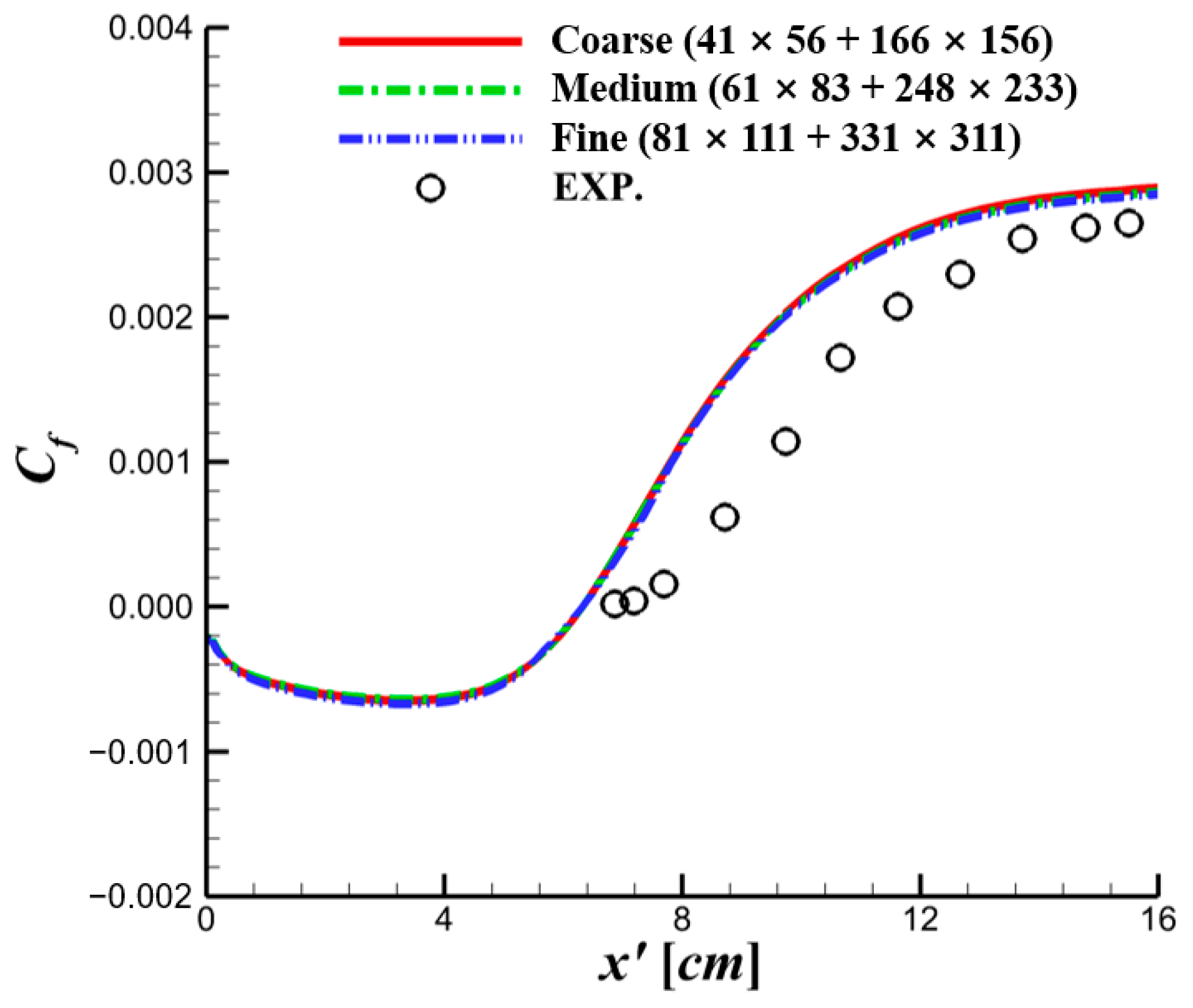
+ ≈ 1 for the wall turbulence simulation. A mesh refinement study using three distinct mesh resolutions (coarse, medium, and fine) is also conducted based on the original SST turbulence model, and the comparison results are presented in Figure 3. As the number of grid points increases, the present CFD results hardly change. For RANS calculations, the baseline grid is already fine enough, and continuing to refine the mesh has a minimal-to-negligible effect on the computational results.
Figure 4 and Figure 5 show the computational results from different turbulence models with and without compressibility corrections. For all the original RANS models, the corrections have a very significant effect on the numerical calculations and significantly improve the distributions of the pressure, skin friction coefficient, and velocity profiles. The original k–ω and BSL models hardly give reasonable computational results, predicting too small recirculation zones. Moreover, the velocity profiles in the shear layer and the distributions of the wall pressure and skin friction coefficient show large deviations from the experiment. Without a compressibility correction, the SST model, in general, gives the closest calculation results to the experiment when compared to the original k–ω and BSL models, but there are still some deviations. For all RANS models considered in present study, generally, the compressibility correction “C2” gives better results than “C1”. The velocity profiles and the wall pressure distribution are closer to those in the experiment, but the skin friction coefficients predicted by the correction “C2” are a little lower than those predicted by the correction “C1”, which shows the influence of different compressibility corrections on the RANS computation.
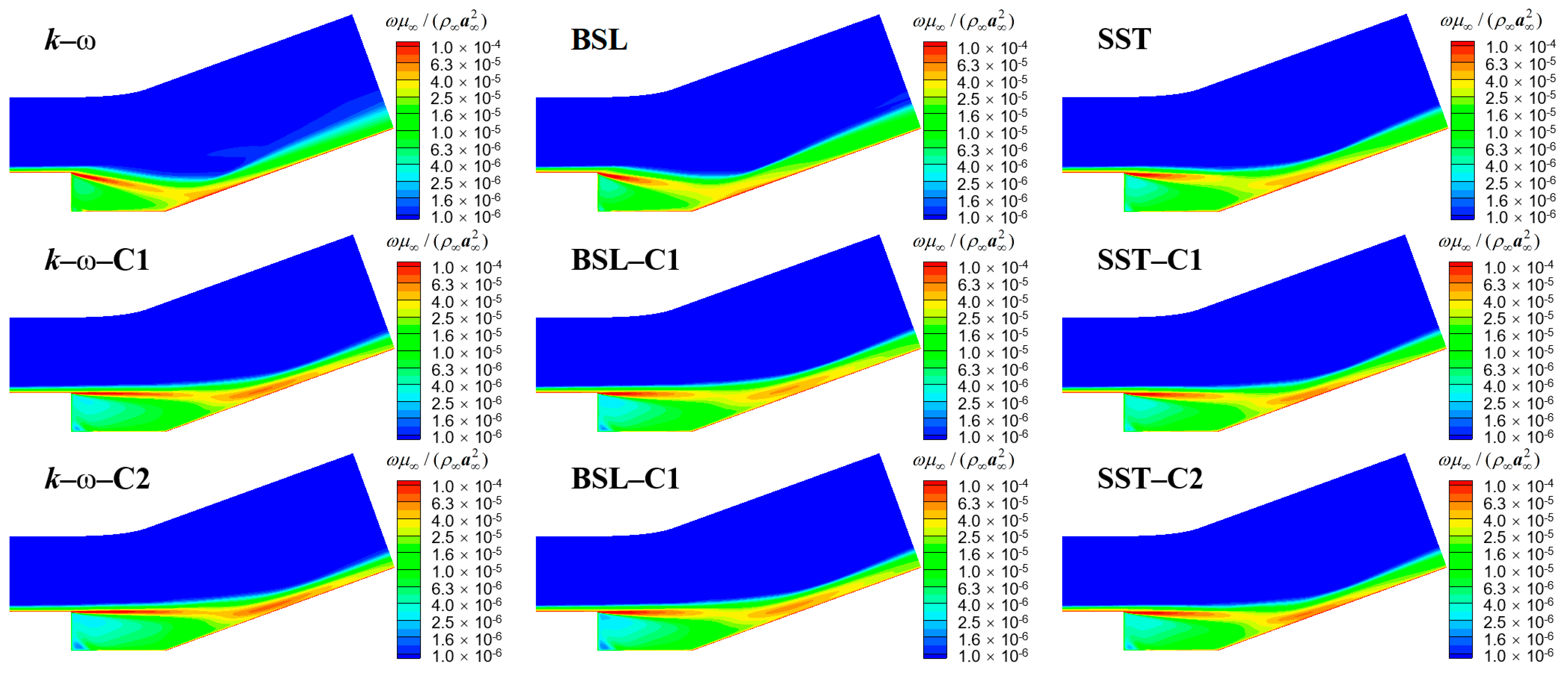
Figure 6 and Figure 7 show the distributions of the turbulent kinetic energy, k, and specific dissipation rate, ω, respectively. The depicted k and ω are nondimensionalized using the free-stream variable values. In the reattachment region, the original RANS models without corrections give very high levels of turbulent kinetic energy. Obviously, compressibility corrections reduce the levels of turbulent kinetic energy in this region, as shown in Figure 6. In addition, the levels of the specific dissipation rate in both the separated shear layer and the reattachment region are slightly increased by the compressibility corrections, as shown in Figure 7. 
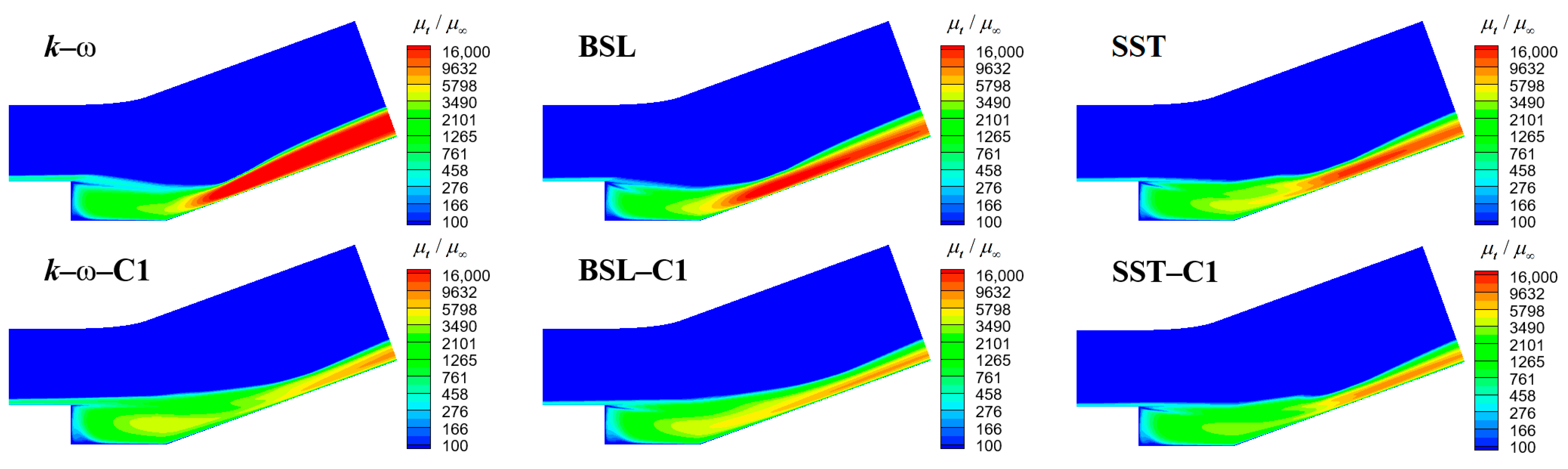
Figure 8 shows the distributions of the turbulent viscosity for the different turbulence models. Compared to the SST model, the original k–ω and BSL models have very high values of turbulent viscosity in the reattached boundary layer. It is difficult to significantly improve the model’s performance with only a single compressibility correction. Therefore, the rapid compression fix and Wilcox’s correction (or Suzen and Hoffmann’s correction) are used in combination for both the original k–ω and BSL models. It can be seen from Figure 8 that the compressibility corrections generally reduce the model’s turbulent viscosity, which has a significant effect on the prediction of flow reattachment and the subsequent boundary layer development. In general, the effect of the correction “C2” is more pronounced than that of “C1”, which can be inferred from the lower levels of turbulent viscosity.
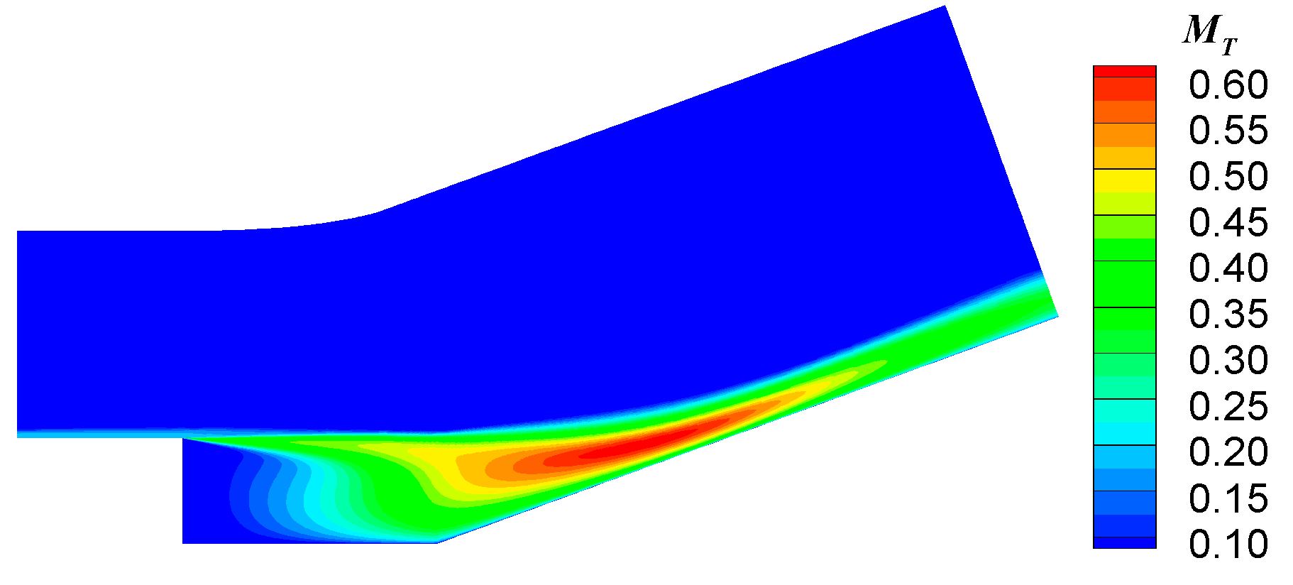
Figure 9 shows the turbulence Mach number distribution in the ramped cavity flow. In addition to the separated shear layer, the turbulence Mach number in the regions of flow reattachment and the subsequent reattached boundary layer close to the wall easily exceeds 0.25. Despite the introduction of the turbulence Mach number threshold in the F(MT) function, the low-speed flow regions close to the wall are still subject to the effect of the compressibility correction. For both corrections (Wilcox’s correction and Suzen and Hoffmann’s correction), the action area and intensity of the compressibility corrections can be illustrated by the contours of functions F(MT)(1 − F1) and (MT)2(1 − F1), respectively. With the introduction of the blending function, F1, Wilcox’s compressibility correction is limited to high-speed flow regions, such as the separated shear layer and the subsequent reattached boundary layer far away from the wall, as shown in Figure 10a. In the case of Suzen and Hoffmann’s compressibility correction, the correction area is roughly the same as that for Wilcox’s correction, but the range is slightly enlarged and the correction intensity is slightly increased, as shown in Figure 10b. As for Suzen and Hoffmann’s correction, the pressure dilatation term also acts almost in the same regions as the dilatation dissipation term. In the action regions, the pressure dilatation term is negative, which, like the effect of the dilatation dissipation term, reduces the turbulent kinetic energy, k, and increases the value of ω, thus reducing the turbulent viscosity of the model. As for the rapid compression fix (not used in the SST model), the velocity divergence, ∇·V, can be used to indicate the action area, as shown in Figure 10c. In Equation (10), ∇·V < 0 or ∇·V > 0 will increase or decrease the production term in the ω-equation of RANS models. In the compression region (near the oblique shock wave), the value of the velocity divergence is less than zero, which directly leads to an increase in w. From Equation (4), the increase in w is an important reason for the decrease in turbulent viscosity. In the expansion region (near the step), the value of the velocity divergence is larger than zero, which directly leads to a decrease in w. Nevertheless, the expansion is weak and has a very limited effect on w. Although these three compressibility corrections are very different, they cause the same effect on the original RANS models, that is, an overall reduction in the turbulent viscosity of the model. The original RANS models always produce too high levels of turbulent viscosity in the non-equilibrium region after separation and overestimate the initial spreading rate of the free shear layer. An adaptive reduction in the turbulent viscosity through compressibility corrections slows down this spreading rate. The overall lower levels of turbulent viscosity in the correction “C2”, when compared to the correction “C1”, are responsible for the better predictions.

3.2. Supersonic Compression Corner Flow

Shock/boundary layer interactions (SBLIs) are a fundamental phenomenon that is widely present in the internal and external flows involved in supersonic vehicles. A classic SBLI phenomenon can be found in supersonic compression corner flows. Settles et al. [30] conducted a series of experiments on this flow at different corner slopes in a 20 × 20 cm-high Reynolds-number channel at Princeton University and obtained reliable experimental data, which can be used for the present numerical validation. The reference experimental data in the subsequent comparisons are taken from this reference [30]. A compression corner is a typical test case for many turbulence models’ performance evaluations in the simulation of supersonic turbulent separated flows.
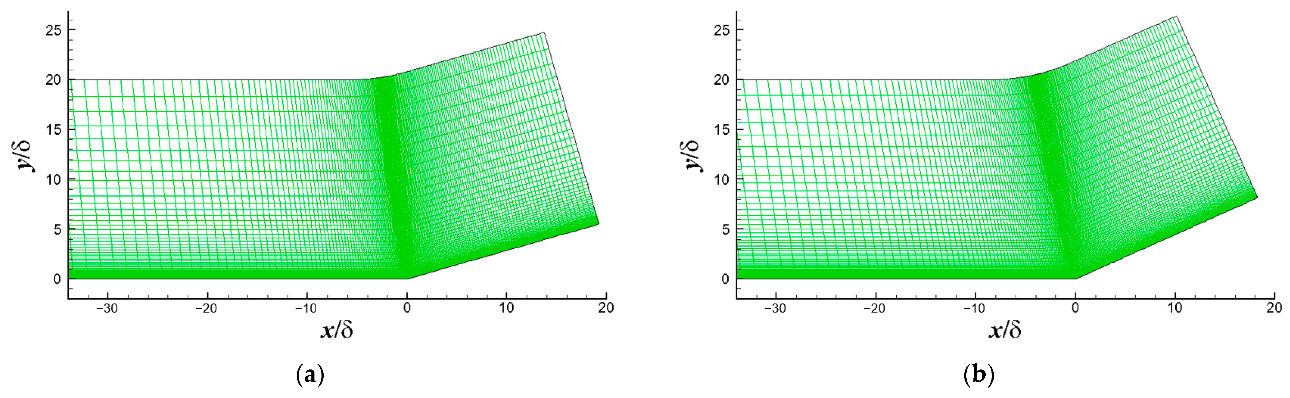
At a 16° corner angle, due to the adverse pressure gradient generated by a shock wave, flow separation starts to occur at the corner, but its range is so small that it is almost unobservable, as shown in Figure 11a. As the corner angle increases, the adverse pressure gradient is gradually enhanced, and the separated region is further expanded. At 24°, the extent of the separation region is almost several times the thickness of the incoming boundary layer, as shown in Figure 11b. Despite the simplicity of the compression corner geometry, the prediction of the supersonic flow separation at large corner angles is a great challenge for conventional RANS models due to the complexity of SBLI as well as its intrinsic unsteadiness. In the present study, two corner angles (16° and 24°) are selected to test and evaluate the RANS models with different compressibility corrections. The computational incoming flow conditions are shown in 
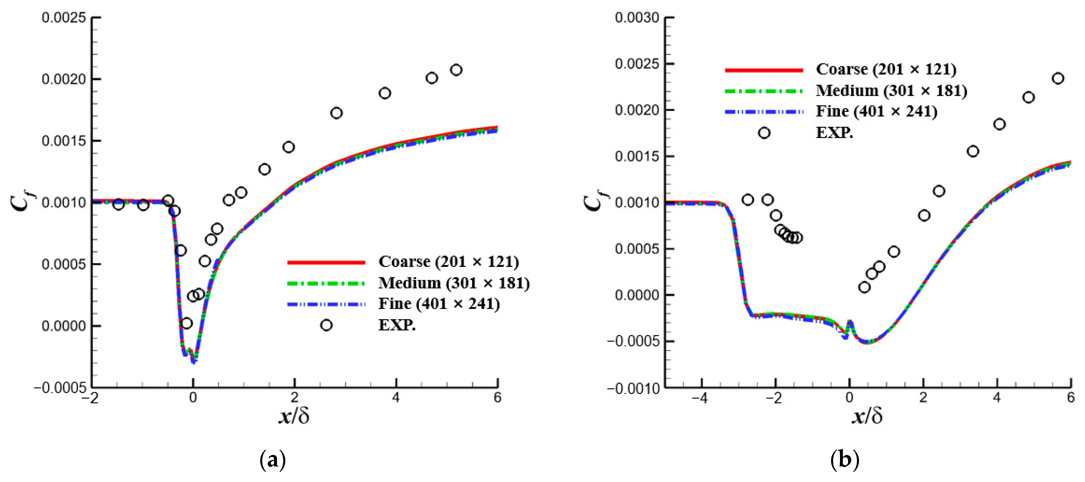
Table 2, and the reference station is twice the thickness of the incoming boundary layer upstream of the corner. For the baseline computational grid, 201 × 121 grid nodes in one structured block are adopted, as shown in Figure 12. Both of the 2D Princeton cases use a wall spacing of 5 × 10⁻⁵δ, resulting in y+ < 1 upstream of both the corners. A mesh refinement study using three distinct mesh resolutions (coarse, medium, and fine) is also performed based on the SST model, and the refinement has little effect on the numerical results, as shown in Figure 13.
The turbulence Mach number distribution for the compression corner flows is shown in Figure 14. At the 16° corner angle, the turbulence Mach number of the entire flow field is roughly less than 0.25, as shown in Figure 14a. The region of high turbulence Mach number is very close to the wall. Under the shielding effect of the blending function F1, Wilcox’s correction and Suzen and Hoffmann’s correction, which are based on the turbulence Mach number, MT, hardly work for the RANS models. Instead, the rapid compression fix plays a major role in the corrections. At the 24° corner angle, it can be seen from Figure 14b that the turbulence Mach number is higher than the threshold, MT0 = 0.25, after flowing through the shock wave. The maximum turbulence Mach number is about 0.45 in the recirculation region at the corner. Even near the wall region, the turbulence Mach number has a large value. Under the shielding effect of the blending function F1, the action region of dilatation dissipation and pressure dilatation in the compressibility corrections is constrained away from the wall, which significantly minimizes the detrimental effect of corrections on the prediction of low-speed flows near the wall.
Similar to the simulation of supersonic ramped cavity flows, the velocity divergence, ∇·V, is used to indicate the action area of the rapid compression fix, as shown in Figure 15. As mentioned previously, this compressibility correction is near the oblique shock wave and will increase the separation bubble size predicated by the original k–ω or BSL model. The contours of the functions F(MT)(1 − F1) and (MT)2(1 − F1) are used to illustrate the action area and the intensity of both Wilcox’s correction and Suzen and Hoffmann’s correction, respectively. For the 24° compression corner flow, a local function value of F(MT)(1 − F1) and (MT)2(1 − F1) greater than zero indicates that the compressibility correction plays a role in this region, and the larger the function value, the more pronounced the correction. As can be seen in Figure 16, the local function values are overall less than 0.08 with Wilcox’s correction, whereas with Suzen and Hoffmann’s correction, there exists a large region of local function values of about 0.1. Suzen and Hoffmann’s correction acts on a larger region than Wilcox’s correction, and the correction is more intense.
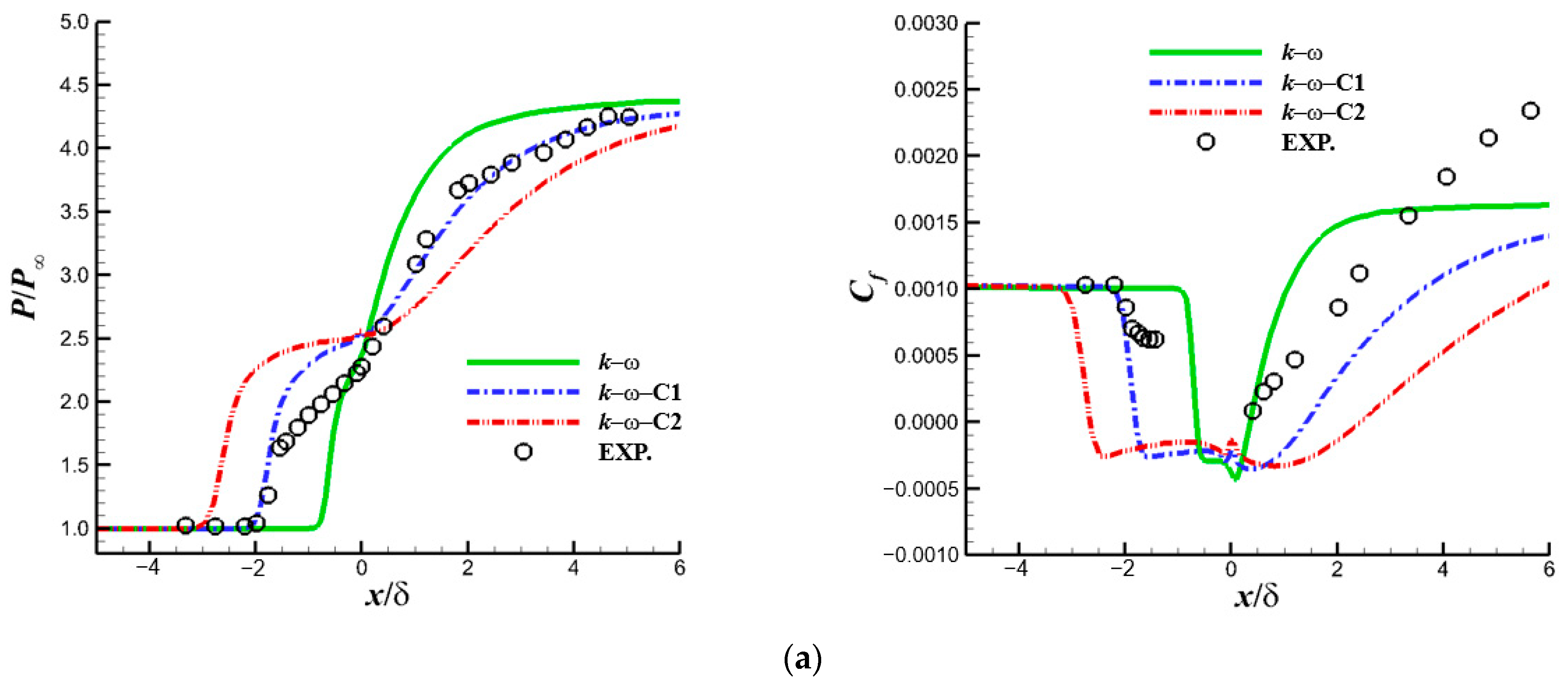
Figure 17 and Figure 18 show the computational results of the wall pressure and skin friction coefficient from the different turbulence models with and without compressibility corrections. At 16°, almost only the rapid compression fix works, which is not introduced in the SST model. Therefore, the calculation results from the SST model with and without corrections are almost identical. Moreover, the calculation results from the two corrections (“C1” and “C2”) for the k–ω and BSL models are also almost the same. However, the compressibility corrections reduce the skin friction coefficient on the ramped surface when compared to the original k–ω and BSL models without corrections. At 24°, a flow separation at the corner is evident with high turbulence Mach number values in the near-wall region; thus, the terms pressure dilatation and dilatation dissipation in the compressibility corrections play a major role in this supersonic turbulent separated flow. There is a difference between the effects of the two compressibility corrections on the calculation results. It can be seen from the numerical results that the effect of the correction method “C2” is too pronounced, which leads to a too large separation region and an obviously low skin friction coefficient distribution on the ramp. In contrast, the correction “C1” has very little effect on the prediction based on the SST model but increases the predicted separation region by the k–ω and BSL models and improves the prediction of the wall pressure distribution. Overall, compared with the experimental data, the compressibility correction “C1” is more favorable than “C2” for the prediction of supersonic compression corner flows. Even based on the SST model, the correction “C1” does not lead to particularly bad result If based on the original k–ω model or BSL model, the correction “C1” can give relatively reasonable predictions for wall pressure distributions and separation point locations close to experimental results.
It should be noted that the SST model does not always give the best predictions for compression corner flows. Bradshaw’s assumption in the SST model may be invalid, or the model constant, a1, may need to be recalibrated for this type of supersonic flow. Compressibility corrections to the SST model instead give worse results at a large corner angle, whereas corrections to the BSL model lead to improved predictions, which have also been confirmed by Forsythe et al. [15]. On the other hand, when the shock-unsteadiness modification is applied to the k–ε, k–ω, and Spalart–Allmaras turbulence models, improved predictions can also be obtained, as shown in the numerical comparisons performed by Sinha et al. [16]. However, the shock-unsteadiness modification is not based on the turbulence Mach number. This modification is not as elegant as Wilcox’s correction and Suzen and Hoffmann’s correction, both of which are based on the turbulence Mach number. Tu et al. [22] introduced Catris’ modification in the SST model equations and obtained improved predictions for the 34° compression corner flow at a Mach number of 9.22. Catris’ modification brings benefits for hypersonic compression corner flows, whereas for supersonic compression corner flows with Mach numbers less than 3, this modification may not have much effect on the computational results.
Figure 19 and Figure 20 show the profiles of turbulent kinetic energy and specific dissipation rate, respectively, at five stations for the 16° compression corner flow. The compressibility corrections “C1” and “C2” have almost no impact on the calculation results of the SST model but have almost exactly the same effect on the results from both the original k–ω and BSL models, since only the rapid compression fix works. The distributions of the turbulent kinetic energy and specific dissipation rate within the boundary layer upstream of the separation point are almost unaffected by the compressibility corrections. At the three stations downstream of the separation point, the peak value of the turbulent kinetic energy decreases due to the rapid compression fix. At the two stations x/δ = 0 and x/δ = 1, the specific dissipation rate is overall increased by the correction. Thus, the turbulent viscosity of both the original k–ω and BSL models is reduced, which is helpful for the prediction of a flow separation with an adverse pressure gradient.
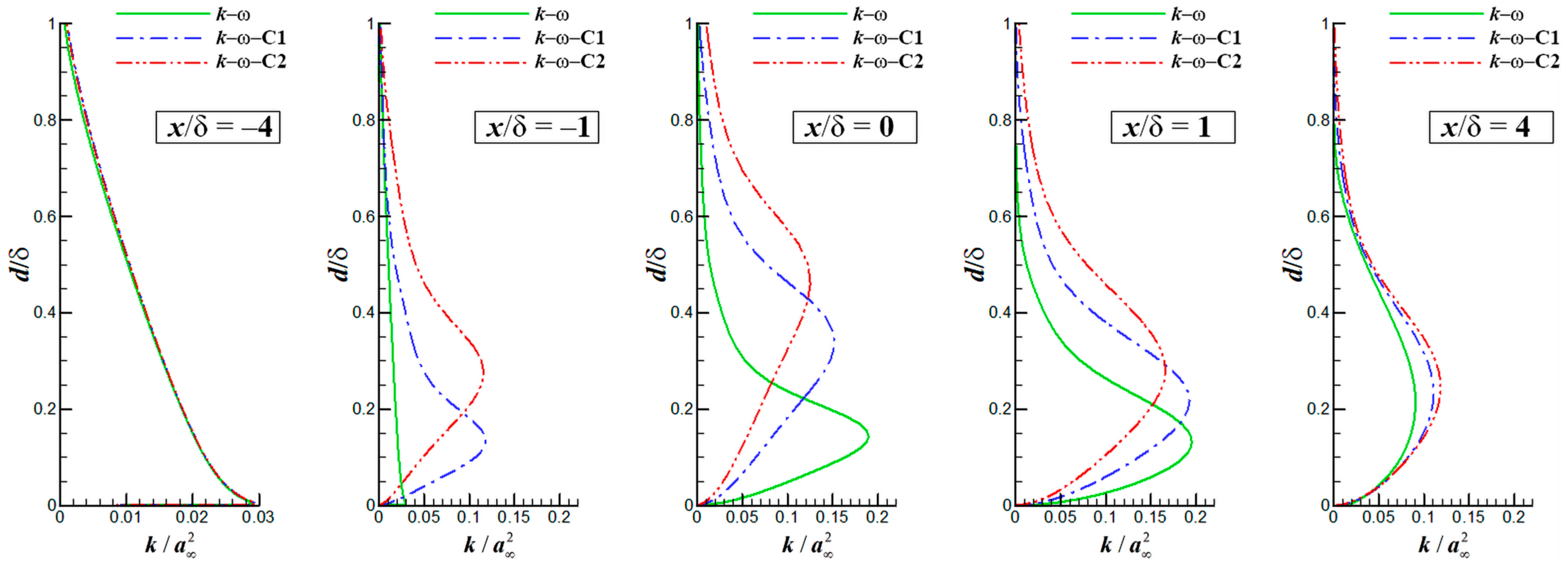
Figure 21 and Figure 22 show the distributions of turbulent kinetic energy and specific dissipation rate, respectively, for the 24° compression corner flow. Due to the high levels of turbulence Mach numbers, not only the rapid compression fix but also Wilcox’s and Suzen and Hoffmann’s corrections authentically work. There is a difference in the effects of the two compressibility corrections, “C1” and “C2”. Similarly, from a comparison of the profiles at the station x/δ = −4, it is clear that the corrections have no effect on the flow prediction in the upstream turbulent boundary layer. In the recirculation region (x/δ = −1~1), the peak values of turbulent kinetic energy are reduced by the corrections. At the station x/δ = −1, the original k–ω and BSL models predict very low levels of turbulent kinetic energy, which is due to the delayed separation. On the other hand, at the station x/δ = 4, larger peak values of turbulent kinetic energy are obtained when the compressibility corrections are adopted, especially for the original k–ω and BSL models. This is due to the fact that more turbulent kinetic energy convects downstream as the separation bubble size increases. As for the specific dissipation rate distribution, in the upper part of the boundary layer, away from the wall and separated shear layer, the specific dissipation rate increases overall after the compressibility correction. In the lower part of the boundary layer, near the wall, the specific dissipation rate decreases overall after the correction. The specific dissipation rate shows a large variation in the direction normal to the wall within the boundary layer, especially when the rapid compression fix is applied.
Figure 23 shows the turbulent viscosity distribution for the compression corner flows. The original k–ω and BSL models have very high turbulent viscosity levels. It is obvious to see that the compressibility corrections significantly reduce the overall turbulent viscosity of the two turbulence models. At 16°, the turbulent viscosity of the SST model is almost unchanged with the corrections since the corrections hardly work at low turbulence Mach numbers. However, when the rapid compression fix is in action, it decreases the turbulent viscosity of both the original k–ω and BSL models. At 24°, the correction “C2” decreases the turbulent viscosity of the turbulence models more when compared to the correction “C1” because Suzen and Hoffmann’s correction is more significant than Wilcox’s correction, which is shown in Figure 16. An excessive reduction in the turbulent viscosity leads to an increase in the separation zone and a decrease in the wall skin friction coefficient downstream of the flow reattachment, which will deteriorate the predictions of the original RANS model. As for the compression corner flows at a large corner angle, the adaptive regulation of the turbulent viscosity in the correction “C1” is more favorable than that in the correction “C2”, because RANS models with the correction “C1” enhance the original models’ sensitivity to adverse pressure gradients without unduly reducing the turbulent viscosity.

4. Conclusions

In the present work, different versions of the k–ω turbulence model were adopted with compressibility corrections. The rapid compression fix combined with Wilcox’s or Suzen and Hoffmann’s correction, which is denoted as “C1” or “C2”, is very effective for both the original k–ω and BSL models. Wilcox’s and Suzen and Hoffmann’s corrections without the rapid compression fix are adopted for the SST model, and they are denoted as “C1” and “C2”, respectively. The computational results before and after the correction for each turbulence model are presented and compared to the available experimental data in detail, using two types of typical supersonic turbulent flows with separation, namely, the ramped cavity flow and the compression corner flow, as test cases. This paper not only shows the positive effects of compressibility corrections but also emphasizes their negative effects. The following conclusions are obtained from this study:
(1) For the supersonic ramped cavity flow, which is dominated by a free shear layer, in general, the present compressibility corrections significantly improve the computational results of the original turbulence model. Suzen and Hoffmann’s compressibility correction, which considers the effects of both dilatation dissipation and pressure dilatation, reasonably predicts the development rate of the separated shear layer. In comparison, Wilcox’s compressibility correction, on the other hand, does not match the experimental values as well as Suzen and Hoffmann’s correction, although it improves the prediction of separated shear layers by the original turbulence models without corrections.
(2) For the supersonic compression corner flow, which is dominated by a turbulent boundary layer, the compressibility correction “C1” is more favorable than the correction “C2” for the prediction of flow separations because the correction “C2” predicts a too large separation region and an obviously low skin friction coefficient distribution. The SST model, which is usually considered to have better performance, does not give satisfactory results. The present compressibility corrections do not improve the prediction results of the SST model and can even be detrimental if the compressibility correction “C2” has been adopted. On the other hand, the compressibility correction “C1” significantly improves the predictions of the k–ω and BSL models, which is confirmed by the reasonable distributions of wall pressure and separation point location close to the available experimental results.
(3) Compressibility corrections reduce the overall turbulent viscosity of the original turbulence model, enlarge the separation region, and slow down the spreading rate of the free shear layer, but they may have a negative impact on the prediction of low-speed flows in the near-wall region, such as significantly reducing the values of the wall skin friction coefficient. Although the blending function F1 can protect the flow in the near-wall region from compressibility corrections, its role is after all limited. Thus, it is recommended that a more suitable near-wall shielding function be introduced in the corrections. Compared with the correction “C2”, the correction “C1” tends to be conservative and at least does not have significant negative effects. However, for the prediction of compressible free shear layers, the correction “C2” is recommended.

Funding

This research received no external funding.

Data Availability Statement

Data are contained within the article.

Conflicts of Interest

The author declares no conflict of interest.

References

  1. Fang, J.; Yao, Y.; Zheltovodov, A.A.; Li, Z.; Lu, L. Direct numerical simulation of supersonic turbulent flows around a tandem expansion-compression corner. Phys. Fluids 2015, 27, 125104. [Google Scholar] [CrossRef]
  2. Slotnic, J.; Khodadoust, A.; Alonso, J.; Darmofal, D.; Gropp, W.; Lurie, E.; Mavriplis, D. CFD Vision 2030 Study: A Path to Revolutionary Computational Aerosciences; NASA/CR–2014-218178; National Aeronautics and Space Administration: Hampton, Virginia, USA, 2014.
  3. Sarkar, S. The pressure–dilatation correlation in compressible flows. Phys. Fluids A Fluid Dyn. 1992, 4, 2674–2682. [Google Scholar] [CrossRef]
  4. Zeman, O. Dilatational dissipation: The concept and application in modeling compressible mixing layers. Phys. Fluids A Fluid Dyn. 1990, 2, 178–188. [Google Scholar] [CrossRef]
  5. Wilcox, D.C. Dilatation-dissipation corrections for advanced turbulence models. AIAA J. 1992, 30, 2639–2646. [Google Scholar] [CrossRef]
  6. Wilcox, D.C. Turbulence Modeling for CFD, 3rd ed.; DCW Industries: La Canada, CA, USA, 2006. [Google Scholar]
  7. Suzen, Y.B.; Hoffmann, K.A. Investigation of supersonic jet exhaust flow by one-and two-equation turbulence models. In Proceedings of the 36th Aerospace Sciences Meeting & Exhibit, Reno, NV, USA, 12–15 January 1998. [Google Scholar]
  8. Horstman, C.C.; Settles, G.S.; Williams, D.R.; Bogdonoff, S.M. A reattaching free shear layer in compressible turbulent flow. AIAA J. 1982, 20, 79–85. [Google Scholar] [CrossRef]
  9. Fan, T.C.; Tian, M.; Edwards, J.R.; Hassan, H.A.; Baurle, R.A. Validation of a hybrid Reynolds-averaged/large-eddy simulation method for simulating cavity flameholder configurations. In Proceedings of the 31st AIAA Fluid Dynamics Conference & Exhibit, Anaheim, CA, USA, 11–14 June 2001. [Google Scholar]
  10. Luo, D.; Yan, C.; Wang, X. Computational study of supersonic turbulent-separated flows using partially averaged Navier-Stokes method. Acta Astronaut. 2015, 107, 234–246. [Google Scholar] [CrossRef]
  11. Yan, C.; Xu, Y.; Cao, R.; Piao, Y. Investigation of very large eddy simulation method for applications of supersonic turbulent combustion. Aerospace 2023, 10, 384. [Google Scholar] [CrossRef]
  12. Tong, F.; Yu, C.; Tang, Z.; Li, X. Numerical studies of shock wave interactions with a supersonic turbulent boundary layer in compression corner: Turning angle effects. Comput. Fluids 2017, 149, 56–69. [Google Scholar] [CrossRef]
  13. Li, X.; Fu, D.; Ma, Y.; Liang, X. Direct numerical simulation of shock/turbulent boundary layer interaction in a supersonic compression ramp. Sci. China Phys. Mech. Astron. 2010, 53, 1651–1658. [Google Scholar] [CrossRef]
  14. Rizzetta, D.P.; Visbal, M. Application of large-eddy simulation to supersonic compression ramps. AIAA J. 2002, 40, 1574–1581. [Google Scholar] [CrossRef]
  15. Forsythe, J.R.; Hoffmann, K.A.; Damevin, H.-M. An assessment of several turbulence models for supersonic compression ramp flow. In Proceedings of the 29th AIAA Fluid Dynamics Conference, Albuquerque, NM, USA, 15–18 June 2001. [Google Scholar]
  16. Sinha, K.; Mahesh, K.; Candler, G.V. Modeling the effect of shock unsteadiness in shock/turbulent boundary-layer interactions. AIAA J. 2005, 43, 586–594. [Google Scholar] [CrossRef]
  17. Wilcox, D.C. Reassessment of the scale determining equation for advanced turbulence models. AIAA J. 1988, 26, 1299–1310. [Google Scholar] [CrossRef]
  18. Menter, F.R. Zonal two equation k-ω turbulence models for aerodynamic flows. In Proceedings of the 24th AIAA Fluid Dynamics Conference, Orlando, FL, USA, 6–9 July 1993. [Google Scholar]
  19. Menter, F.R. Two-equation eddy-viscosity turbulence models for engineering applications. AIAA J. 1994, 32, 1598–1605. [Google Scholar] [CrossRef]
  20. Catris, S.; Aupoix, B. Improved turbulence models for compressible boundary layers. In Proceedings of the 2nd AIAA Theoretical Fluid Mechanics Meeting, Albuquerque, NM, USA, 15–18 June 1998. [Google Scholar]
  21. Catris, S.; Aupoix, B. Density corrections for turbulence models. Aerosp. Sci. Technol. 2000, 4, 1–11. [Google Scholar] [CrossRef]
  22. Tu, G.; Deng, X.; Mao, M. Assessment of two turbulence models and some compressibility corrections for hypersonic compression corners by high-order difference schemes. Chin. J. Aeronaut. 2012, 25, 25–32. [Google Scholar] [CrossRef]
  23. Coratekin, T.; van Keuk, J.; Ballmann, J. Performance of upwind schemes and turbulence models in hypersonic flows. AIAA J. 2004, 42, 945–957. [Google Scholar] [CrossRef]
  24. Vuong, S.T.; Coakley, T.J. Modeling of turbulence for hypersonic flows with and without separation. In Proceedings of the 25th AIAA Aerospace Sciences Meeting, Reno, NV, USA, 24–26 March 1987. [Google Scholar]
  25. Brown, J.L. Turbulence model validation for hypersonic flows. In Proceedings of the 8th AIAA/ASME Joint Thermophysics and Heat Transfer Conference, St. Louis, MO, USA, 24–26 June 2002. [Google Scholar]
  26. Xiao, X.; Hassan, H.A.; Edwards, J.R.; Gaffney, R.L., Jr. Role of turbulent Prandtl numbers on heat flux at hypersonic Mach numbers. AIAA J. 2007, 45, 806–813. [Google Scholar] [CrossRef]
  27. Huang, P.G.; Coakley, T.J. Turbulence modeling for complex hypersonic flows. In Proceedings of the 31st Aerospace Sciences Meeting & Exhibit, Reno, NV, USA, 11–14 January 1993. [Google Scholar]
  28. Settles, G.S.; Baca, B.K.; Williams, D.R.; Bogdonoff, S.M. A study of reattachment of a free shear layer in compressible turbulent flow. In Proceedings of the 13th AIAA Fluid & Plasma Dynamics Conference, Snowmass, CO, USA, 14–16 July 1980. [Google Scholar]
  29. Settles, G.S.; Williams, D.R.; Baca, B.K.; Bogdonoff, S.M. Reattachment of a compressible turbulent free shear layer. AIAA J. 1982, 20, 60–67. [Google Scholar] [CrossRef]
  30. Settles, G.S.; Fitzpatrick, T.J.; Bogdonoff, S.M. Detailed study of attached and separated compression corner flowfields in high Reynolds number supersonic flow. AIAA J. 1979, 17, 579–585. [Google Scholar] [CrossRef]
Figure 1. Sketch of the supersonic ramped cavity flow.
Aerospace 10 01014 g001
Figure 2. Computational grid.
Aerospace 10 01014 g002
Figure 3. Mesh refinement study for the supersonic ramped cavity flow.
Aerospace 10 01014 g003
Figure 4. Plots of surface pressure (left) and skin friction coefficient (right) for the ramped cavity.
Aerospace 10 01014 g004
Figure 5. Velocity profiles in shear layer for turbulence models with and without compressibility considerations.
Aerospace 10 01014 g005
Figure 6. Turbulent kinetic energy distribution for RANS models with and without compressibility corrections.
Aerospace 10 01014 g006
Figure 7. Specific dissipation rate distribution for RANS models with and without compressibility corrections.
Aerospace 10 01014 g007
Figure 8. Turbulent viscosity distribution for RANS models with and without compressibility corrections.
Aerospace 10 01014 g008aAerospace 10 01014 g008b
Figure 9. Distribution of turbulence Mach number for the ramped cavity flow.
Aerospace 10 01014 g009
Figure 10. Comparison of the area where a compressibility correction works for the ramped cavity flow: (a) Wilcox’s correction; (b) Suzen and Hoffmann’s correction; (c) rapid compression fix.
Aerospace 10 01014 g010
Figure 11. Sketch of the supersonic compression corner flow: (a) 16°; (b) 24°.
Aerospace 10 01014 g011
Figure 12. Computational grid for the supersonic compression corner flow: (a) 16°; (b) 24°.
Aerospace 10 01014 g012
Figure 13. Mesh refinement study for the supersonic compression corner flow: (a) 16°; (b) 24°.
Aerospace 10 01014 g013
Figure 14. Distribution of turbulence Mach number for the compression corner flows: (a) 16°; (b) 24°.
Aerospace 10 01014 g014
Figure 15. Action area of rapid compression fix for the compression corner flows: (a) 16°; (b) 24°.
Aerospace 10 01014 g015
Figure 16. Comparison of the area where a compressibility consideration works for the 24° compression corner flow: (a) Wilcox’s correction; (b) Suzen and Hoffmann’s correction.
Aerospace 10 01014 g016
Figure 17. Plots of surface pressure (left) and skin friction coefficient (right) for the 16° supersonic compression corner: (a) original k-ω models with or without corrections; (b) BSL models with or without corrections; (c) SST models with or without corrections.
Aerospace 10 01014 g017aAerospace 10 01014 g017b
Figure 18. Plots of surface pressure (left) and skin friction coefficient (right) for the 24° supersonic compression corner: (a) original k-ω models with or without corrections; (b) BSL models with or without corrections; (c) SST models with or without corrections.
Aerospace 10 01014 g018aAerospace 10 01014 g018b
Figure 19. Turbulent kinetic energy profiles for the 16° compression corner flow.
Aerospace 10 01014 g019aAerospace 10 01014 g019b
Figure 20. Specific dissipation rate profiles for the 16° compression corner flow.
Aerospace 10 01014 g020aAerospace 10 01014 g020b
Figure 21. Turbulent kinetic energy profiles for the 24° compression corner flow.
Aerospace 10 01014 g021aAerospace 10 01014 g021b
Figure 22. Specific dissipation rate profiles for the 24° compression corner flow.
Aerospace 10 01014 g022aAerospace 10 01014 g022b
Figure 23. Turbulent viscosity distribution for the compression corner flows: (a) 16°; (b) 24°.
Aerospace 10 01014 g023
Table 1. Calculation conditions for the supersonic ramped cavity flow.
MRe/mδ, cmP, PaT, K
2.926.7 × 1070.2921,24095.37
Table 2. Calculation conditions for the supersonic compression corner flow.
Princeton RampsMP0, PaT0, Kδ, mmRe/mReδ
16°2.856.9 × 105268266.56 × 1071.71 × 106
24°2.846.9 × 105262236.83 × 1071.57 × 106
Disclaimer/Publisher’s Note: The statements, opinions and data contained in all publications are solely those of the individual author(s) and contributor(s) and not of MDPI and/or the editor(s). MDPI and/or the editor(s) disclaim responsibility for any injury to people or property resulting from any ideas, methods, instructions or products referred to in the content.

