Oil Particle-Induced Erosion Wear on the Deflector Jet Servo Valve Prestage

Abstract

Severe oil particle-induced erosion to the prestage component progressively degrades the overall performance of the deflector jet servo valve (DJSV), even leading to valve failure. Herein, we present an approach for evaluating degradation in performance and predicting the erosion lifespan of the DJSV on different levels of oil pollution. Specifically, a mathematical model of the whole valve was built based on a previously established working principle and physical mechanism. In addition, considering the horizontal and rotational particle motions, combined with impact of particle size distributions under different oil contamination degrees, an erosion model was constructed. Then, after simulating and analyzing the pressure characteristics before and after the erosion of prestage, the performance degradation of the whole valve was examined, thereby predicting the erosion life of the valve. Investigations revealed that the maximum erosion rate occurred at the shunt wedge of the receiving holes, which increased with the contamination degree and accelerated after level 7. After erosion, however, the control pressure difference decreased significantly, and erosion life followed exponential distribution corresponding to the distribution of particles under different pollution levels. The aforementioned investigation can thus help diagnose faults and optimize the design of the servo valves in service.

1. Introduction

The electric–hydraulic servo valve serves as the key component of the hydraulic system, particularly in aerospace that primarily determines the reliability and safety of the entire hydraulic system. Statistics shows that oil contamination is the primary fault factor for the servo valve, accounting for about 70% of the total fault, while the erosion wear caused by the particles in oil is one of the main types of failure [1,2,3,4]. The DJSV, as a typical servo valve, is developed on the basis of jet pipe valve, and it has been widely employed in aerospace and other operations owing to its high dynamic response and anti-pollution performances [5,6]. However, the prestage component is a critical component of the valve. Because of the special structure in the prestage, the contamination particles in the oil still would introduce significant erosion to the prestage, which eventually deteriorates the overall performances of the DJSV gradually and hence necessitates a deeper literary insight into the prestage erosion wear [7].

Solid particle erosion is a complex process, and its underlying mechanism is not fully understood today. A general model of measurement, revealing material erosion entirely and comprehensively, does not exist [8,9]. The experimentally validated E/CRC and Oka models are highly cited among other contemporary studies for the erosion wear of servo valve [10,11]. Based on E/CRC and Oka models, previous studies on the erosion of valve by the particles in oil, mainly focused on the impact of erosion on leakage for valve and impact of particle size, velocity, collision angle and structure size. Based on the deformation of E/CRC erosion model, Li et al. [2] investigated the impact of erosion wear on the leakage within the valve and proposed a new performance degradation analysis model for linear hydrostatic actuator. Zhang et al. [12] examined the jet flapper servo valve wear caused by oil contamination, internal leakage effects, weakening pressure and gain linearity. Based on CFD, Ji et al. [13] researched the erosion of prestage for a DJSV. The results revealed that the erosion rate decreased along the rising of the displacement, the angle of the V-shaped window and the thickness of the deflector. Used E/CRC erosion model by Yan et al. [14] researched the erosion wear on a jet pipe valve. The findings demonstrated that most serious erosion was on the wedge and a direct relationship exists between the diameter of solid particles and the erosion rate. Yan [15] used the Oka model to simulate the erosion of the prestage, and found that the erosion can be divided into four levels and if the lifetime of a valve exceeded 20,000 h, then the contamination level of oil must be guaranteed at NAS 5. Chu [16] established the valve performance degradation model and completed the life prediction. Combined with Amesim software, Meng [17] analyzed the influence of prestage erosion wear on the working performance of the whole valve. However, the previous studies have not considered particle size distributions under different levels of oil pollution. In addition, only a few researchers have conducted a quantitative analysis of the differential pressure change in prestage and its influence on the performance of the whole valve after erosion.

Therefore, this study presents a method for analyzing the characteristic degradation and predicting the erosion lifespan about DJSV on different levels of oil pollution. First, we introduced the operating principle about the DJSV, after which the mathematical model based on the whole valve was built. Next, the erosion model was constructed for oil contamination, comprising the horizontal and rotational movements of particles and their related forces (e.g., the rotational lift force [Magnus force] caused by rotation), after which the impact of particle size distributions under different oil contamination degrees was assessed. Then, we used two typical erosion rate calculation models, the E/CRC and the Oka, to compare and analyze the prestage erosion wear by simulating in an ANSYS environment, in addition to the pressure changes after erosion. Subsequently, the performance degradation of the whole valve was also analyzed by combining the theoretical analysis with the erosion simulation results, followed by a final prediction of the erosion life of the valve.

2. Theory and Mathematical Models

2.1. Working Principle of the DJSV

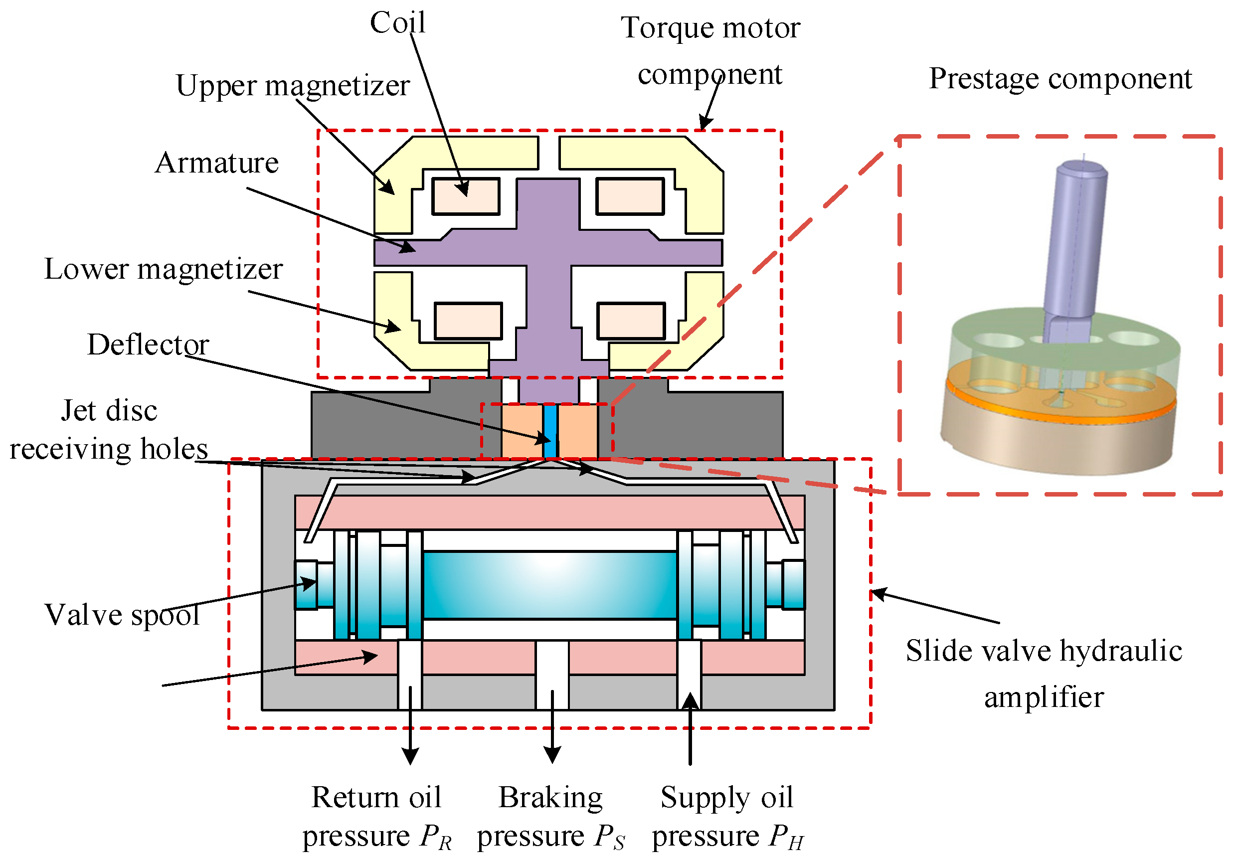
The DJSV incorporates torque motor component, prestage component, and slide valve hydraulic amplifier. Figure 1 illustrates a schematic workflow of the DJSV where the input is a low current signal to the coil which drives the armature assembly, performing the force conversion and movement functions. Subsequently, the prestage realizes the conversion of displacement and pressure through the jet. In the end, the pressure difference of the receiving holes drives the slide valve to move. Oil under high pressure reaches braking chamber as the core valve is moved toward the right, increasing braking pressure. On the contrary, when the core valve is moved toward the left, the brake cavity is connected with the return oil, and at the same time the high-pressure oil supply port is closed. Therefore, the oil flows out of the brake cavity and the brake pressure is reduced.

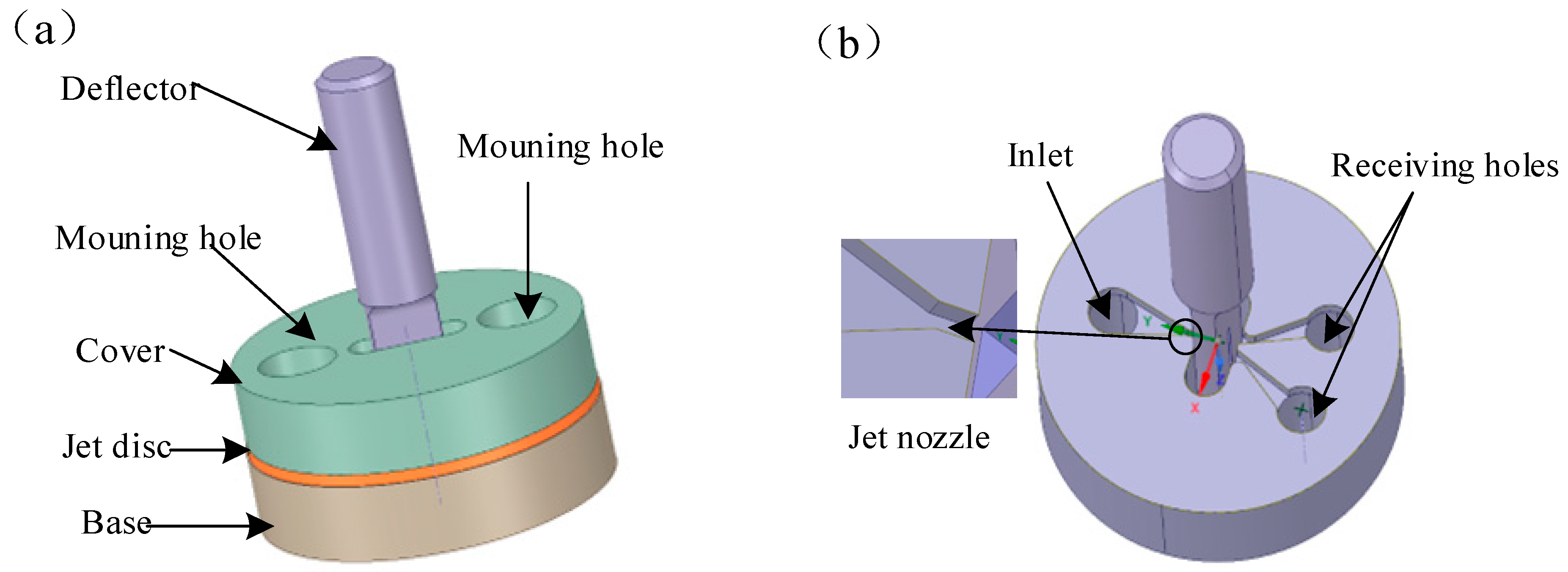
Figure 2 shows the detailed architecture of the prestage component. The jet disc is fixed between the cover and base with closed plenum chamber at the upper and lower ends. The deflector is combined and installed between nozzle and receiver. The oil flows to the jet nozzle generating a free jet that eventually passes through the V-shaped slit channel inside the deflector, and finally reaches two separate receiving holes that extend to the slide valve’s control chambers at each end. The cavity between the nozzle and the receiver is connected to the oil return line. In practice, the erosion wear could be problematic since the oil line of pre-stage is narrow, and the flow rate is high.

2.2. Mathematical Model of the Torque Motor

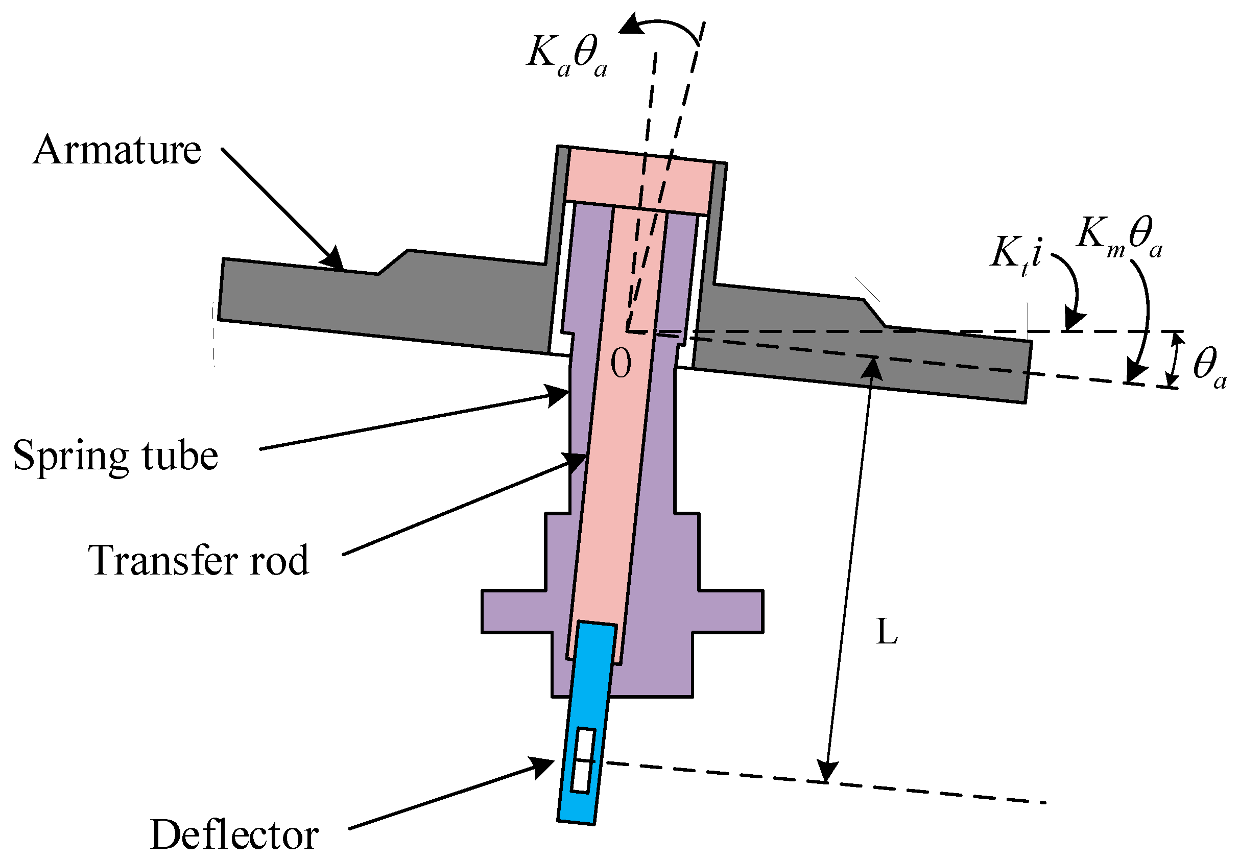
As shown in Figure 3, the armature rotating component is composed of armature, spring tube, transfer rod and deflector. Upon inputting current into the armature’s control coil, an electromagnetic moment $T_m$ is produced when an armature rotates under electromagnetic force:

$$T_m=K_{t}i+K_m{\theta }_a$$

(1)

where $K_{t }$is the median electromagnetic torque coefficient of torque motor, $K_m$ is the electromagnetic spring stiffness of the torque motor, and ${\theta }_a$ is the rotation angle.

With armature rotating, the transfer rod and deflector are driven to rotate together, while the lower part of the spring tube is not moved, and the upper part is deformed. The dynamic balance equation of the armature rotating component is shown as below:

$$T_m=J_a{s}^2{\theta }_a+B_{a}s{\theta }_a+K_a{\theta }_a$$

(2)

where$J_{a }$and $B_a$ represent the moment inertia and viscous damping coefficient, respectively, about armature, transfer rod and deflector. $K_a$ represents spring tube’s stiffness.

The deflector rotates along with the armature. The displacement is $x_f$, which can be calculated as follows:

$$x_f=L{\theta }_a$$

(3)

where L represents distance from the center of V-shaped slit channel inside the deflector to the rotation center O.

2.3. Prestage Amplifier Model

The movement of the deflection plate causes the pressure difference between the two receiving holes, which drives the slide valve to move forming flow rate and pressure. Therefore, the prestage realizes the conversion of displacement and pressure through the jet. The relation between the control pressure difference and displacement of the deflector is given as below:

$$\Delta P=K_p{x}_f$$

(4)

where$K_{p }$is pressure difference amplification factor of prestage.

2.4. Mathematical Model of Slide Valve

The spool moves under the action of forces to realize the conversion from mechanical motion to pressure. There are several forces involved in this movement, including the differential pressure in control and feedback chambers, the reset spring’s force, damping forces, hydraulic forces and spool–sleeve friction. Dynamic balance equation for the slide valve can be expressed as follow:

$$\Delta P{A}_v-(P_S-P_R)A_f=m_v{S}^2{x}_v+B_{v}S{x}_v+K_v{x}_v+F_f$$

(5)

where $A_v$ and $A_f$ represent the areas of control and feedback cavity, respectively, $x_v$ represents displacement for the valve, m_v represents valve core quality, $B_v$ represents the damping coefficient of the main spool includes the damping generated by transient hydraulic force, $K_v$ represents the stiffness coefficient of the servo valve including reset spring stiffness and stable hydraulic stiffness, $F_f$ represents the friction caused by the lateral force, $P_R$ represents pressure of back oil and $P_S$ represents braking pressure.

The transient hydraulic force $F_W=0.43W\Delta P_1{x}_v$. The stable hydraulic force $F_{ss}=L{C}_{q}W\sqrt{2\rho \Delta P_1}S{x}_v$. The velocity and flow coefficient is $C_q$, the fluid density is $\rho$, the area gradient at the opening of valve is W, the distance between the inlet and outlet of a valve is measured by L, and pressure difference between pre- and post-valve ports is $\Delta P_1$.

When the brake cavity is connected with high-pressure oil, the oil enters into the brake chamber. On the contrary, when the brake cavity is connected with the return oil, the oil flows out of the brake cavity. So that the fluid can be illustrated as below:

$$\begin{array}{l}{Q}_s=C_{sq}W(x_v-x_0)\sqrt{\frac{2}{\rho }(P_H-P_S)}\hspace{1em}\hspace{1em}{x}_v-x_0\ge 0\\ Q_s=C_{sq}W(x_v-x_0)\sqrt{\frac{2}{\rho }(P_S-P_R)}\hspace{1em}\hspace{1em}{x}_v-x_0<0\end{array}$$

(6)

where $C_{sq}$ is the flow coefficient at valve port, $P_H$ is pressure on oil supply, and $x_0$ is valve core overlap with valve sleeve.

The brake cavity is a closed cavity. The relationship between the flow, volume and the brake pressure can be described as follows:

$$Q_s=\frac{V_t}{E}S{P}_R$$

(7)

where $V_t$ is volume of brake cavity and E is the elastic modulus of oil.

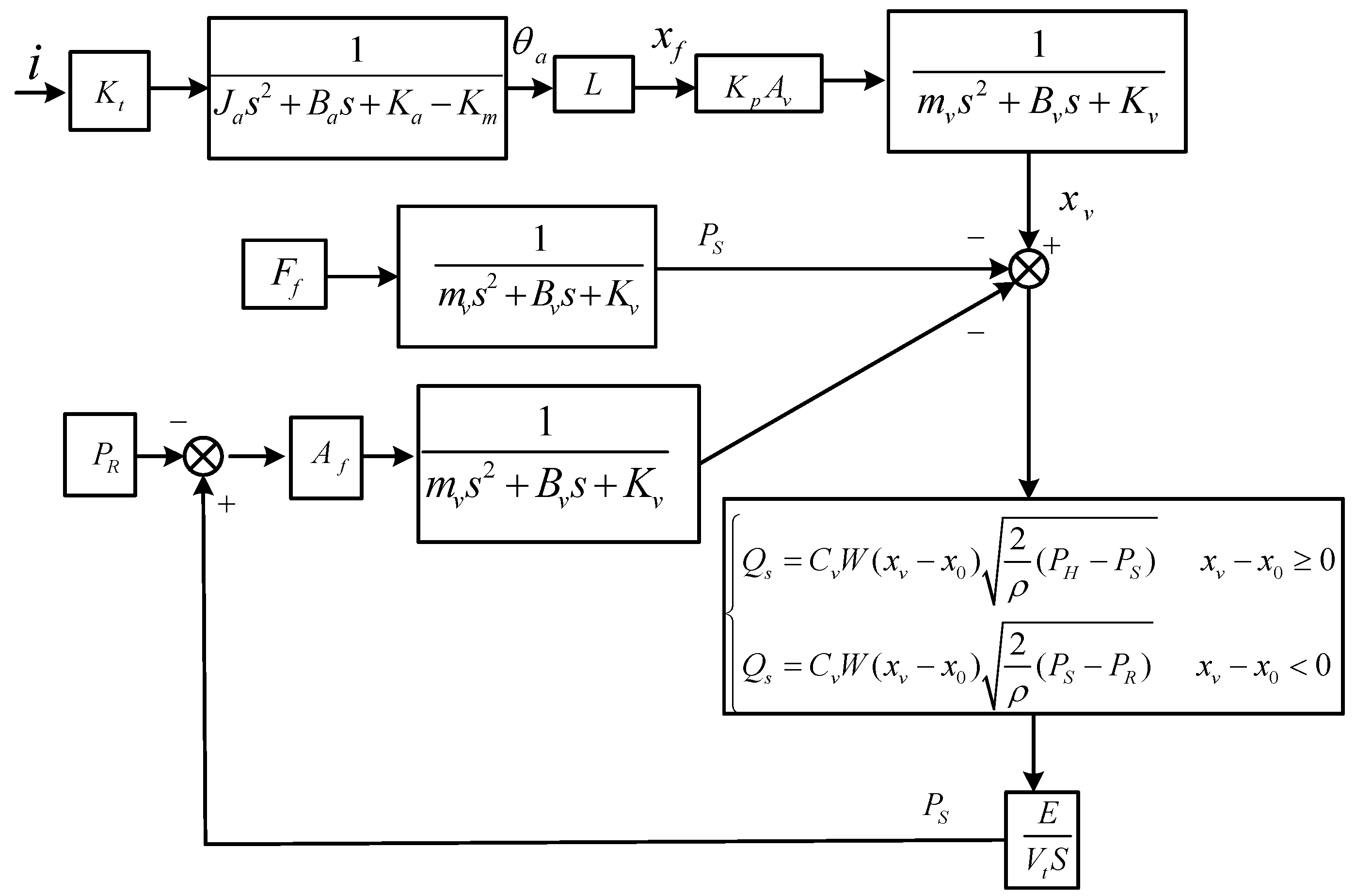
As shown in Figure 4, it is possible to obtain the block diagram of the valve’s dynamic transfer system by synthesizing Equations (1)–(9).

3. Erosion Modeling

In preceding studies, the flow field and particle movements were usually simplified to facilitate the calculation [18]. Specifically, the particle horizontal movement as well as the forces of flow on a particle were considered, while both the particle rotation movement and the forces of the particle on flow were ignored. In this study, a bidirectional coupling between the particles and the flow field is considered while the rotation action about particle and the forces of rotation are contemplated, which makes the established model more consistent with the actual situation.

3.1. Continuous Phase Model

The continuity equations, i.e., the Reynolds-averaged N–S equation and the standard $k-\epsilon$equation models, are accounted to model the continuous phase.

The continuous equation for incompressible fluid is given as:

$$\nabla ·(\rho \overrightarrow{V})=0$$

(8)

where $\overrightarrow{V}$ is the velocity vector of the fluid.

The continuous phase could be modeled using the N–S equations as follows:

$$\frac{D(\rho \overrightarrow{V})}{Dt}=-\nabla P+\mu {\nabla }^2\overrightarrow{V}+\rho \overrightarrow{g}+\nabla ·{\overrightarrow{\tau }}_{ij}+{\overrightarrow{F}}_P$$

(9)

where P is the static pressure, μ is the dynamic viscosity of the fluid, $\overrightarrow{g}$ is the acceleration of gravity, ${\overrightarrow{\tau }}_{ij}$ is the Reynolds stress tensor, and ${\overrightarrow{F}}_P$ is the interaction force between the fluid and the particles.

The Standard $k-\epsilon$ equation is as below established by Shih et al. [19]:

$$\frac{\partial (\rho k)}{\partial t}+\nabla \rho k\overrightarrow{V}=\nabla ·(\mu +\frac{{\mu }_t}{{\sigma }_k})\nabla k+G_k-\rho \epsilon +S_{\mathrm{p}}^k$$

(10)

$$\frac{\partial (\rho \epsilon )}{\partial t}+\nabla \rho \epsilon \overrightarrow{V}=\nabla ·(\mu +\frac{{\mu }_t}{{\sigma }_{\epsilon }})\nabla \epsilon +C_1{G}_k-\rho C_2\frac{{\epsilon }^2}{k}+S_P^{\epsilon }$$

(11)

where k is turbulence kinetic energy, ε is turbulence kinetic energy dissipation rate, ${\mu }_t$ is the turbulent viscosity,${\sigma }_k$ is the turbulent Prandtl number of k, ${\sigma }_{\epsilon }$ is the turbulent Prandtl number of $\epsilon$, $S_P^k$and $S_P^{\epsilon }$represent the effects of dispersed phase on turbulent flow structure, $G_k$ is the turbulent kinetic energy induced by the average velocity gradient, $C_1$and $C_2$ are the empirical constants.

3.2. Particle Force Modeling

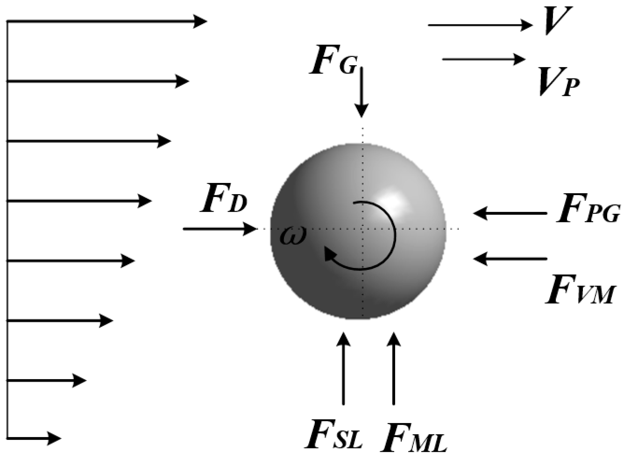
Collective motion of fluid and particles is influenced by fluid forces. Gravity, pressure gradient force, fluid drag force, and virtual mass force are the four main forces. In addition, high-velocity gradients result in unbalanced pressure distributions on particle surfaces, and also generate shear lift, which is also known as Saffman lift [20]. Due to their high moment of inertia, particles that are large and heavy play a significant role in their trajectory. The particle trajectory obtained from the simulation could differ from actual trajectory if the rotation of particles is ignored. Taking into account the rotation moment of the particle and the Magnus force, also called rotational lift, is essential.

The forces acting on a particle by fluid are shown in Figure 5. The force on per unit mass is used in the Equations that follow.

$$\frac{d{\overrightarrow{V}}_P}{dt}={\overrightarrow{F}}_D+{\overrightarrow{F}}_{PG}+{\overrightarrow{F}}_{VM}+{\overrightarrow{F}}_G+{\overrightarrow{F}}_{SL}+{\overrightarrow{F}}_{ML}$$

(12)

where ${\overrightarrow{V}}_P$ represents particle velocity. ${\overrightarrow{F}}_{VM}$ represents virtual mass force. ${\overrightarrow{F}}_D$ represents fluid’s drag force on particle. ${\overrightarrow{F}}_G$ represents gravity. ${\overrightarrow{F}}_{SL}$ represents Shear lift and ${\overrightarrow{F}}_{ML}$ represents Magnus force generated by particle rotation.

For the rotation of particle, an ordinary differential equation about angular momentum needs to be solved. The moment balance equation of particle is shown as below [21]:

$$\overrightarrow{T}=I_p\frac{d{\overrightarrow{w}}_p}{dt}=\frac{\rho }{2}{(\frac{d_P}{2})}^5{C}_r\left|\overrightarrow{\mathsf{\Omega }}\right|\overrightarrow{\mathsf{\Omega }}$$

(13)

where $\overrightarrow{T}$ is the moment acting on the particle, $I_P$ is the moment of inertia about the particle found from $I_p=\frac{\pi }{60}{\rho }_P{\left(\frac{d_P}{2}\right)}^5$ for spherical particle, $d_P$ is diameter of particle, ${\overrightarrow{w}}_{{}_P}$ is the rotational angular velocity of particle, $\Omega =\frac{1}{2}\nabla \times \overrightarrow{V}-{\overrightarrow{w}}_P$ is the relative angular momentum, $C_r$ is the rotating coefficient,

$$C_r=\{\begin{array}{l}\frac{64\pi }{R{e}_r}\hspace{1em}\hspace{1em}R{e}_r\le 32\\ 12.9R{e}_r{}^{-0.5}+128.4R{e}_r{}^{-1}\hspace{1em}\hspace{1em}32<R{e}_r<1000\end{array}$$

(14)

where $R{e}_r$ is the rotational Reynolds number,

$$R{e}_r=\frac{\rho d_P^2\left|\overrightarrow{\mathsf{\Omega }}\right|}{\mu }$$

(15)

In particle motion, drag force ${\overrightarrow{F}}_D$ plays a crucial role. The mathematical relationship can be expressed as below:

$${\overrightarrow{F}}_D=\frac{\overrightarrow{V}-{\overrightarrow{V}}_P}{{\tau }_r}=\frac{18}{24}{C}_D\frac{\mu }{{\rho }_P}\frac{Re}{d_P^2}(\overrightarrow{V}-{\overrightarrow{V}}_P)$$

(16)

where $C_D$ represents factors that influence resistance, ${\tau }_r$ represents time for particle relaxation [22] and Re represents the relative Reynold’s number.

$${\tau }_r=\frac{{\rho }_P{d}_P^2}{18\mu }\frac{24}{C_{D}Re}$$

(17)

$$Re=\frac{\rho d_P\left|\overrightarrow{V}-{\overrightarrow{V}}_P\right|}{\mu }$$

(18)

As a result of fluid pressure distribution around a particle, pressure gradient force ${\overrightarrow{F}}_{PG}$ is generated as follows:

$${\overrightarrow{F}}_{PG}=\frac{\rho }{{\rho }_P}{\overrightarrow{V}}_P\nabla \overrightarrow{V}$$

(19)

When accelerating the movement of the fluid that surrounds a particle, the particle is subjected to an additional force called virtual Force ${\overrightarrow{F}}_{VM}$. Here is the calculation formula:

$${\overrightarrow{F}}_{VM}=\frac{1}{2}\frac{\rho }{{\rho }_P}\frac{d}{dt}(\overrightarrow{V}-{\overrightarrow{V}}_P)$$

(20)

The pressure gradient and virtual mass forces are usually disregarded when fluid density is significantly lower than particle density. However, it is impossible to disregard the pressure gradient and virtual mass forces if density ratio of fluid to particle can be almost 1. When the density ratio is larger than 0.1, it is advised to consider these two forces.

Buoyancy or Gravitational force ${\overrightarrow{F}}_G$ is another factor affecting the motion of particle. It can be mathematically modeled as follows:

$${\overrightarrow{F}}_G=\frac{\left|{\rho }_P-\rho \right|}{{\rho }_P}\overrightarrow{g}$$

(21)

A shear lift force ${\overrightarrow{F}}_{SL}$ acts on a particle when it moves in fluid with a velocity gradient, or alternatively termed as Saffman lift introduced by Mclaughlin [23]. It is mathematically defined as:

$${\overrightarrow{F}}_{SL}=1.615d_p^2{(\frac{\rho \mu }{\overrightarrow{\left|w\right|}})}^{\frac{1}{2}}\left[(\overrightarrow{V}-{\overrightarrow{V}}_P)\times \overrightarrow{w}\right]$$

(22)

where $\overrightarrow{w}=\nabla \times \overrightarrow{V}$ is the velocity curl of the fluid. A corrective element for the lift force Reynolds numbers about larger particle has been developed by Mei [24]:

$${\overrightarrow{F}}_{SL}=1.615d_p^2{(\frac{\rho \mu }{\overrightarrow{\left|w\right|}})}^{\frac{1}{2}}{C}_s\left[(\overrightarrow{V}-{\overrightarrow{V}}_P)\times \overrightarrow{w}\right]$$

(23)

where $C_S$ is a correction factor.

$$C_s=\{\begin{array}{l}(1-0.3314{\beta }^{0.5})e^{-Re/10}+0.3314{\beta }^{0.5}\hspace{1em}\hspace{1em}Re\le 40\\ 0.0524{(\beta Re)}^{1/2}\hspace{1em}\hspace{1em}Re>40\end{array}$$

(24)

where β is a parameter given by $\beta =\frac{1}{2}\frac{R{e}_s}{Re}$ (0.005 < β < 0.4) and $R{e}_s$ is the particle Reynolds number of the shear flow, $R{e}_s=\frac{{\rho }_f{d}_p^2\left|\overrightarrow{w}\right|}{\mu }$.

When a particle rotates in the fluid, an additional lift acting on the particle is known as the Magnus lift or rotational lift ${\overrightarrow{F}}_{ML}$.

$${\overrightarrow{F}}_{ML}=\frac{1}{2}{A}_P{C}_m\rho \frac{\left|\overrightarrow{V}-{\overrightarrow{V}}_P\right|}{\overrightarrow{\mathsf{\Omega }}}(\overrightarrow{\mathsf{\Omega }}\times (\overrightarrow{V}-{\overrightarrow{V}}_p))$$

(25)

where $A_P$ is projected area of particles and $C_m$ is the rotational lift coefficient defined by Oesterle and Dinh [25] as below:

$$C_m=0.45+(\frac{R{e}_r}{Re}-0.45)e^{-0.05684R{e}_r{}^{0.4}R{e}^{0.3}}\hspace{1em}\hspace{1em}Re<2000$$

(26)

Turbulence affects the mobility of particles. The interaction between a fluid vortex and a particle is described using a discrete random walk (DRW) model.

3.3. Particle Recoil Modeling

The particle loses momentum with every collision with the surface wall. The velocity profile ratio after particle collision to that before is known as the recovery coefficient, which measures momentum loss. Typically, different materials are tested to establish the particle rebound model. Depending on the impact of AISI4130 carbon steel and sand particles with diameters of 150–300 μm, an empirical impact model was presented by Forder et al. [26]:

$$e_t=\frac{V_{t2}}{V_{t1}}=1-0.78\theta +0.84{\theta }^2-0.21{\theta }^3+0.028{\theta }^4-0.022{\theta }^5$$

(27)

$$e_n=\frac{V_{n2}}{V_{n1}}=0.988-0.78\theta +0.19{\theta }^2-0.024{\theta }^3+0.027{\theta }^4$$

(28)

where $e_t$ is the tangential rebound coefficient and $e_n$ is the normal rebound coefficient. $\theta$ is the pre-collision angle between particle’s trajectory and container’s surface wall.

$V_{t1}$ and $V_{t2}$ are tangential element of velocity before and after particle–wall collision, respectively. $V_{n1}$ and $V_{n2}$ are the normal element of velocity before and after particle–wall collision, respectively.

The coefficients of tangential and normal rebound provided in Equations (27) and (28) can be used to evaluate the velocity profile after impact.

3.4. Erosion Model

Based on the collision testing on AISI1018 steel [11], the E/CRC model was developed by the Erosion-Corrosion Research Center:

$$ER=C{(HB)}^{-0.59}{F}_S{V}_P^{n}f(q)$$

(29)

$$f(\theta )=a_1\theta +a_2{\theta }^2+a_3{\theta }^3+a_4{\theta }^4+a_5{\theta }^5$$

(30)

where C represents constant of the wall material. $F_S$ represents constant of particle shape. HB represents the value of Brinell Hardness depending on the wall material. As an empirical constant, n represents the index of collision velocity and $f(\theta )$ is the function about the colliding angle. Some other constants given in

Table 1. The related parameters in erosion models.

E/CRC model	C	n	a1	a2	a3	a4	a5
	2.17 × 10−7	2.41	5.4	−10.11	10.93	−6.33	1.42
Oka model	K	k1	k2	k3	V’ (m/s)	D’ (µm)	n1	n2
	65	−0.12	2.3(Hv)0.038	0.19	104	326	0.71(Hv)0.14	2.4(Hv)−0.94

are deduced from a series of direct impact tests of Inconel 718 [27].

After completing studies of numerous test conditions, Oka et al. [12] developed an erosion equation with extra parameters:

$$E R=g (\theta ) \hspace{0.17em}{E}_{90}$$

(31)

$$E_{90}=K{(Hv)}^{k1}{(\frac{V_P}{V^{\prime }})}^{k2}{(\frac{d_P}{D^{\prime }})}^{k3}$$

(32)

$$g(\theta )=(\sin \theta {)}^{n1}{(1+Hv(1-\sin \theta ))}^{n2}$$

(33)

where $E_{90}$ is the volume erosion rate under the normal impact angle, Hv represents the Vickers hardness of the wall material, k1 and k2 depend on the material properties of particle and wall. relative particle diameter D’, K, k3, and relative collision speed V’ rely on the particle’s characteristics. The n1 and n2 are expressed as a function of initial material hardness, which are determined only by the type, shape and property of particles. Table 1 displays related parameter values.

4. Simulation and Numerical Schemes of SPC

CFD-based numerical simulation and erosion estimation are primarily comprised of three components, namely the internal flow field calculations, particle pathway monitoring and erosion rate calculations, respectively. Generally, the fluid’s pressure, speed, and kinetic energy in turbulence can be computed by Reynolds N–S and turbulence models. Subsequently, the Lagrange–Euler method-based discrete phase model is then employed to follow the trajectory of the particles, and pertinent data are captured between the particles and the wall, including collision velocity, impact angle, and location. Finally, with the pertinent parameters acquired in the earlier steps, a suitable erosion model is finally developed to estimate the particle erosion.

4.1. Simulation Modeling

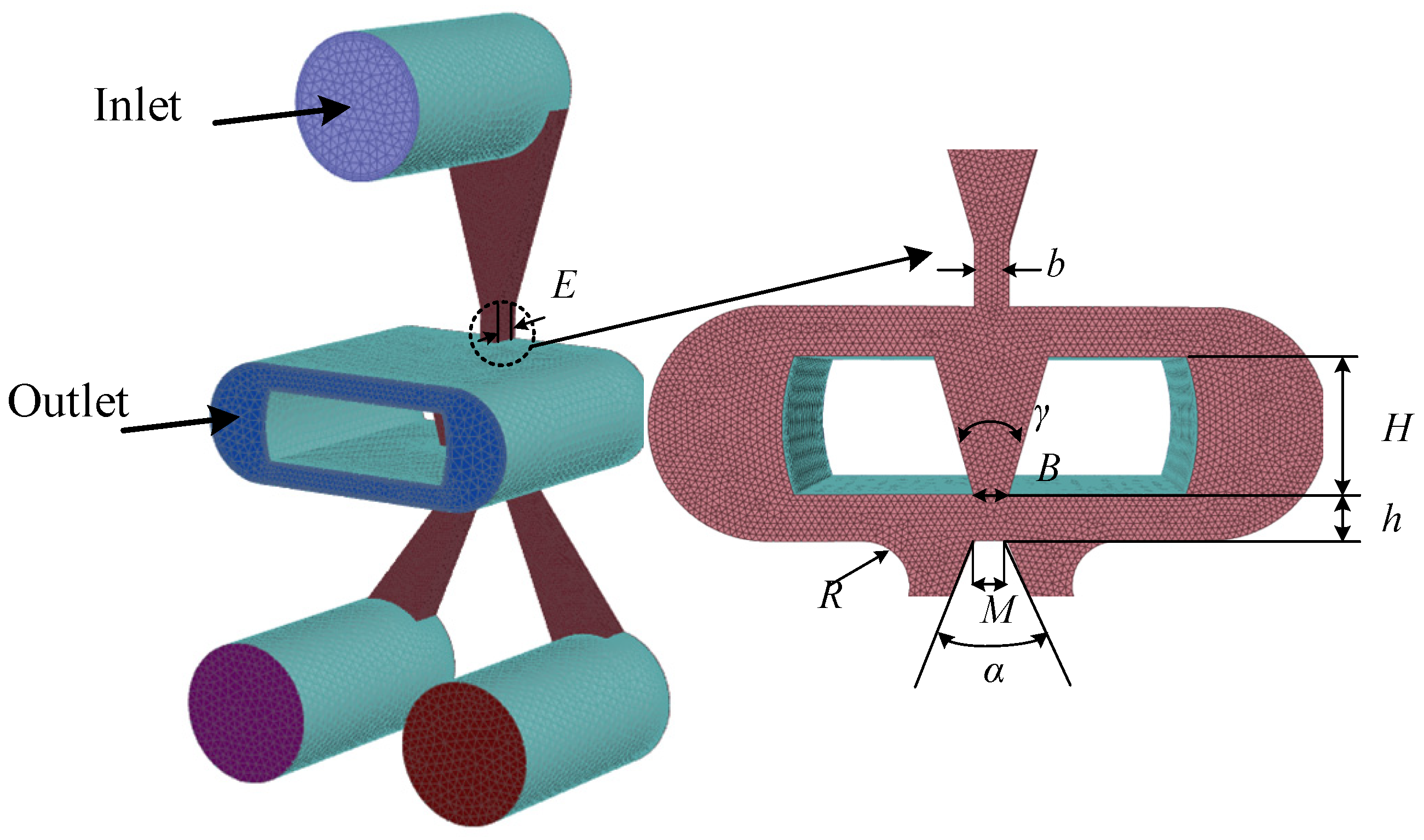
The fluid domain model of the prestage is shown in Figure 6 and the parameters of structure are illustrated in

Table 2. The parameters of structure.

Parameter	Valve
Jet orifice width b	0.15 mm
Outlet width of the deflector B	0.15 mm
Shunt wedge width of receiving holes M	0.14 mm
V-shaped hole length of the deflector H	0.6 mm
Height between deflector outlet andshunt wedge of receiving holes h	0.2 mm
Thickness of jet disc E	0.3 mm
Lateral width of receiving holes R	0.2 mm
V-shaped hole angle of the deflector γ	32°
Angle of receiving holes α	45°

. The most complex flow field is the region from jet orifice to receiving holes. In order to increase simulation accuracy, the mesh at this region is refined, and in addition the FLUENT software is used for simulation. The medium is No. 12 aviation hydraulic oil, the dynamic viscosity is 0.0123 Pa·s, and the density is 850 kg/m³. The density of the particle is 2650 kg/m³, which represents the density of one common pollution particle SiO₂. The boundary conditions of the pressure inlet and outlet are set as 8 MPa and 0.4 MPa, respectively. The convergence precision of the residual error ws set to 10⁻⁵.

4.2. Particle Size Distribution Function

Based on the GJB420B standard, which is classification of particle pollution for aviation working fluid, particles under different contamination degrees were injected. Meanwhile, the Rosin–Rammler distribution function was used to set the parameters of injected particles in the fluent:

$$Y_d=e^{-{(d_p/\overline{d})}^N}$$

(34)

where $Y_d$ was the mass fraction of particles with diameter bigger than $d_p$ in the total particles, $\overline{d}$ was the average particle diameter and N was the size distribution index.

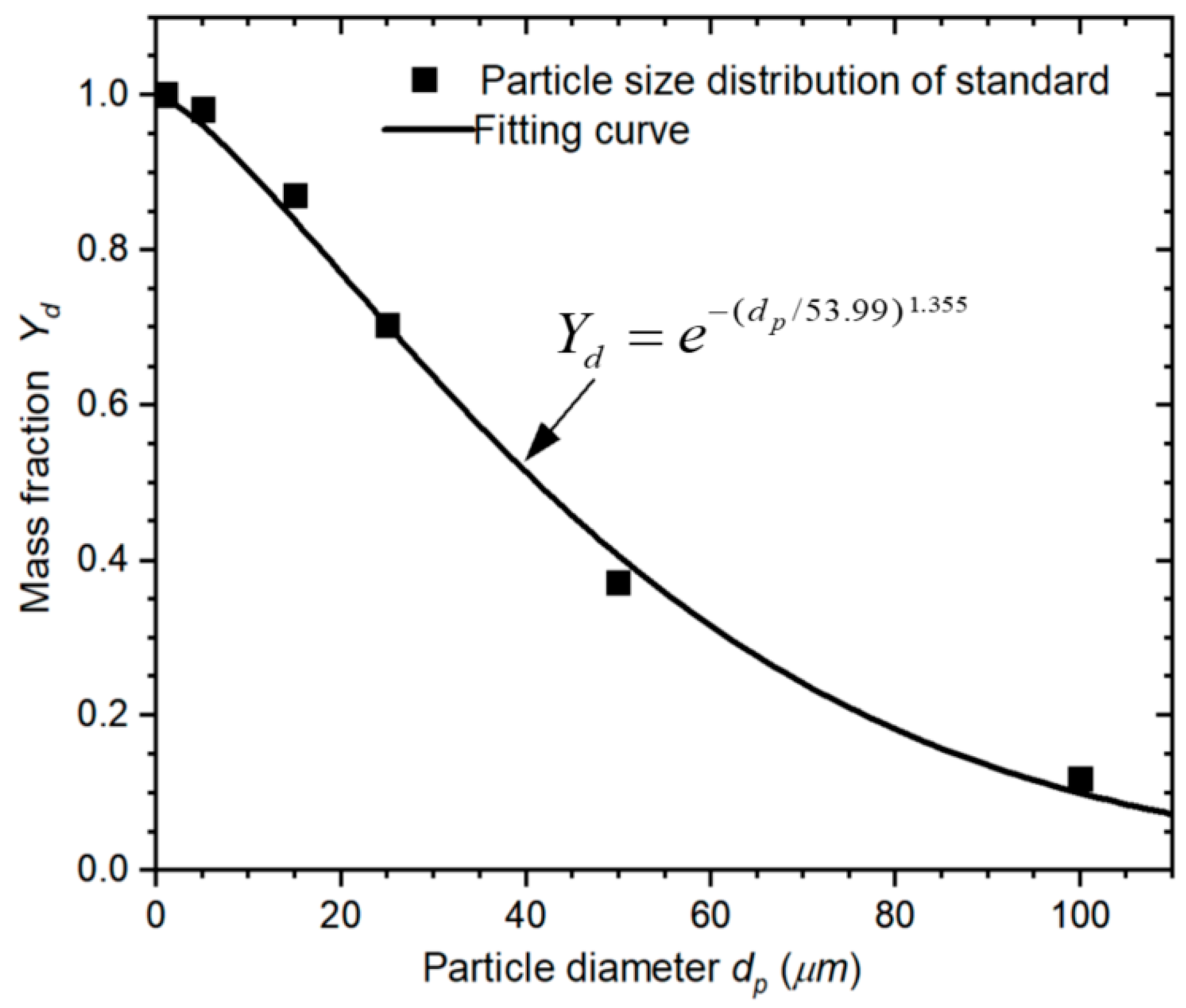
According to the distribution of various particle diameters in level-7 contamination standard, the mass fraction $Y_d$ can be calculated. MATLAB numerical fitting tool with the Rosin–Rammler distribution function was used to obtain the distribution curve of $Y_d$, as shown in Figure 7. Then the average particle diameter and the size distribution index can be obtained, which were 53.99 µm and 1.355, respectively. The average particle diameters and size distribution indices for pollution levels 1, 3, 5, 9, 10, 11, and 12 can be obtained by the same method, which were shown in

Table 3. Rosin–Rammler distribution parameters of particles.

Contamination Degree	1	3	5	7	9	10	11	12
$\overline{d}$ (µm)	65.01	53.81	53.97	53.99	53.95	54	53.93	53.87
N	1.295	1.351	1.356	1.355	1.356	1.357	1.356	1.356

.

5. Result and Discussions

The prestage is a symmetrical structure. When the deflector moves to the left, the process of the jet flow is similar to that of moving to the right. Therefore, the following study takes the deflector moving to the right as an example.

5.1. Pressure under Different Deflector Displacement

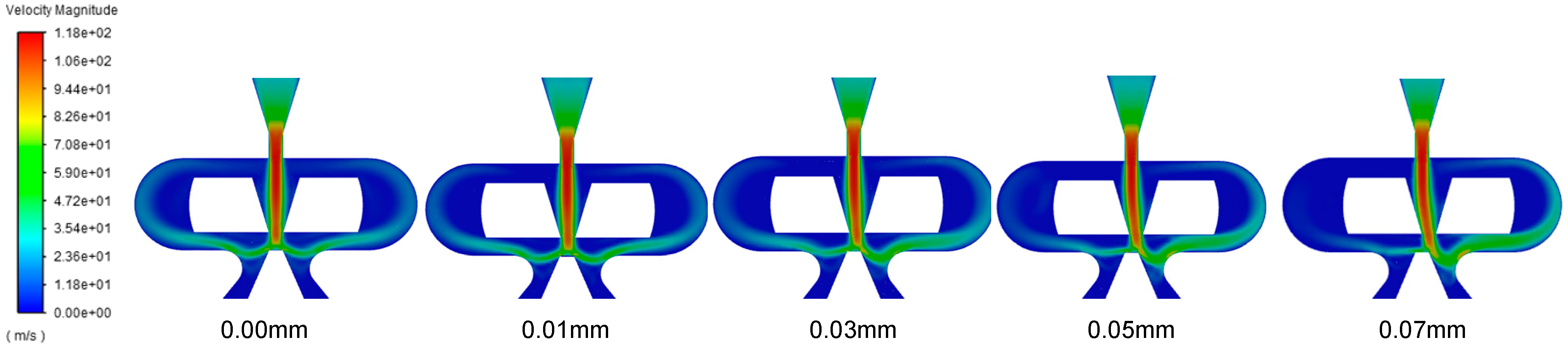
The speed distribution of SPC, with the deflector shifting to the right, is shown in Figure 8. When the oil passed through the jet nozzle with a shrinking channel size, its speed increased rapidly, reaching the highest value of 118 m/s. Then, the high-speed oil passed through the V-shaped slit channel inside the deflector, flowed toward the shunt wedge of the receiving holes, and finally reached the jet’s return outlet. When the deflector moved to right, it showed that the maximum jet velocity almost did not change, the core region of the jet inside the V-slit channel collided with the deflector’s left and deflected to right. As a result, the high kinetic energy at the secondary jet port shifted to the right, thereby decreasing the impact radian of the oil at the left receiving hole and increasing it at the right receiving hole. Therefore, more oil was injected into the right receiving hole, generating pressure difference and promoting the movement of the spool.

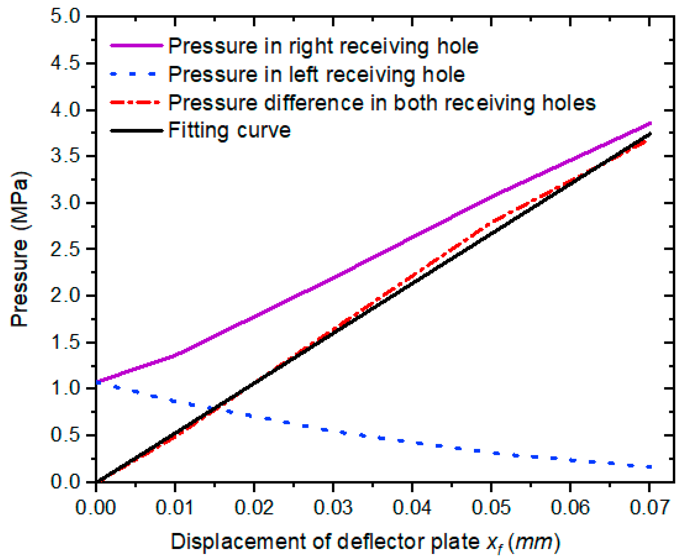
Figure 9 illustrates the pressure and pressure difference in receiving holes with the deflector shifting toward the right. The fitting curve represented the pressure difference $\Delta P=53.55\times {10}^9{x}_f$. Along with the mathematical valve model, the static and dynamic efficiency of the DJSV can be assessed using this fitting formula. As the deflector moved to the right, the pressure of the right receiving hole gradually increased while the left receiving hole gradually decreased. Therefore, the two receiving holes’ pressure difference increased. This corresponded to the velocity distribution under different displacement of deflector.

5.2. Change in Erosion Rate upon Varying Contamination Degrees

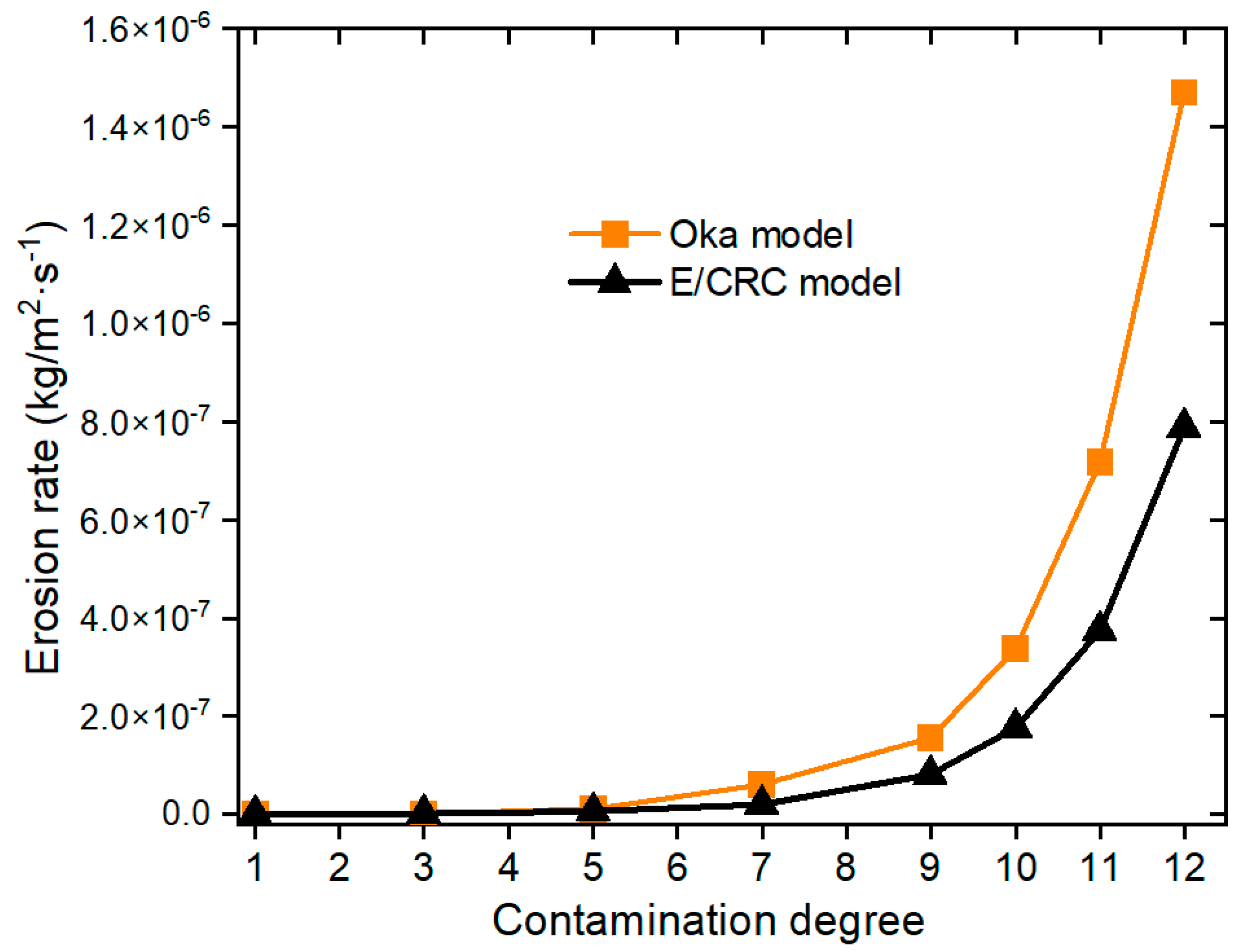
When the deflector was positioned in the jet’s center, the erosion rate was simulated with a rise in pollution levels. According to Figure 10, the erosion rate incremented gradually with the addition of contamination degrees, and the growth rate was faster after level-7. We propose that this event occurred because, in addition to the increase in the number of contamination particles with the level of contamination, the frequency of particle–wall collisions rose, consequently enhancing the erosion growth rate. We also observed that since a larger particle had a greater mass than a smaller particle, the larger kinetic energy under the same speed, density, and hardness, led to significant erosion. Furthermore, smaller particles were more easily affected by turbulence and more sensitive to fluid fluctuations, therefore the momentum exchanges between fluid and particles were more efficient. From the GJB420B standard, the number of large-size particles increased significantly after level-7 contamination degree, so the growth speed of the erosion rate became faster as well. The growth trends of the erosion rate obtained using the E/CRC and Oka models were also consistent under the same conditions, except that the erosion rate for the Oka model was slightly higher than that of the E/CRC model.

5.3. Erosion under Different Deflector Displacement

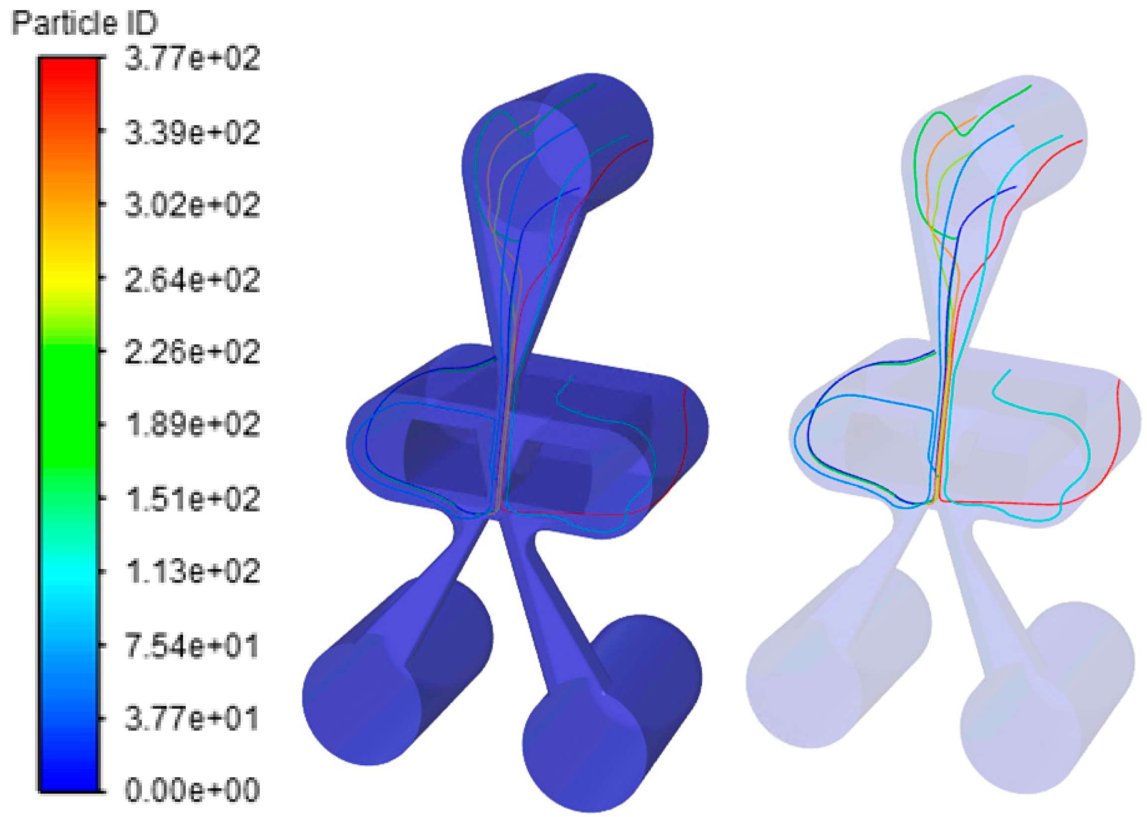
Figure 11 shows the trajectory of the particles, which passed through the V-shaped slit channel of the deflector with high speed, collided with the shunt wedge of receiving holes, and finally reached the return outlet of jet.

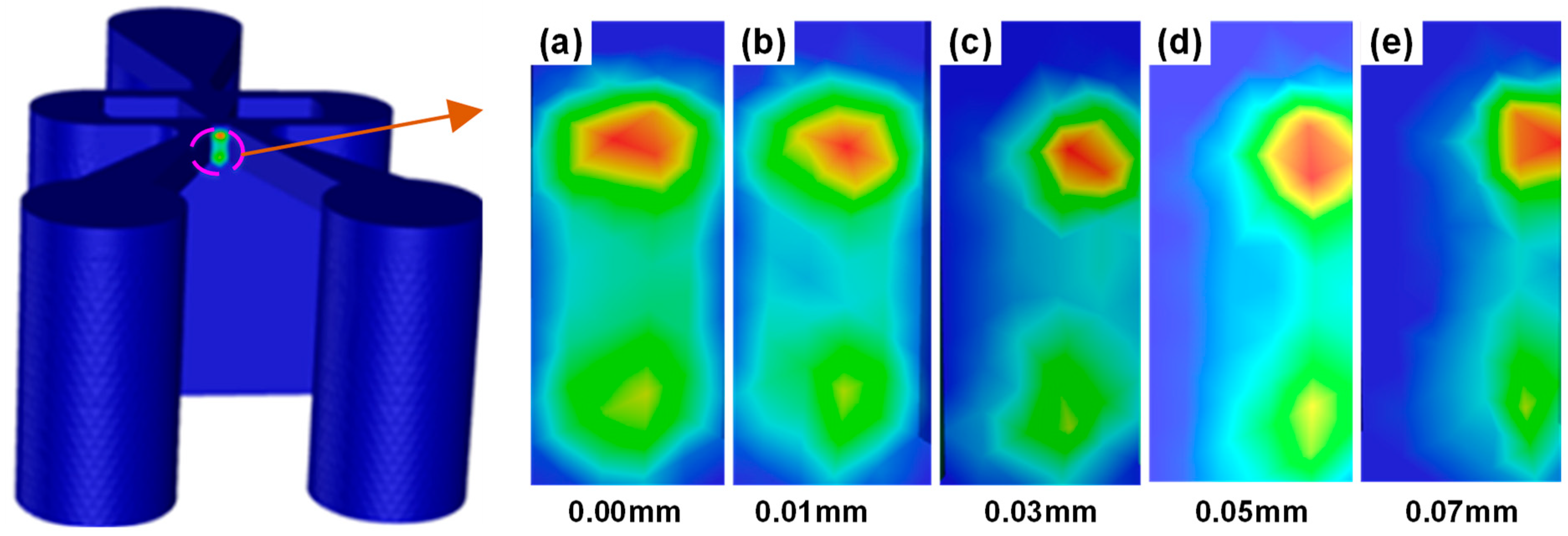
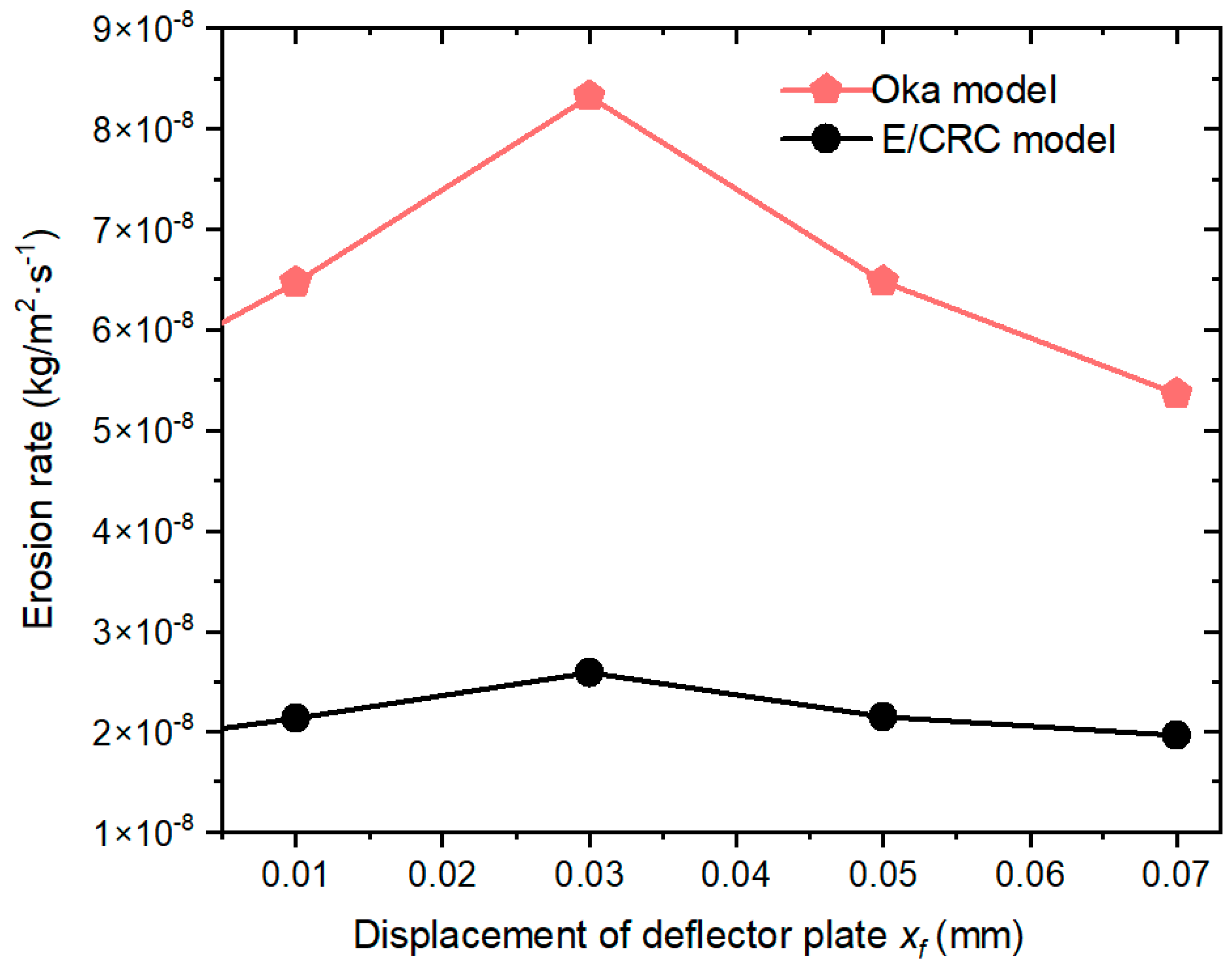
Figure 12 and Figure 13 show the trend corresponding of the erosion rate with the movement of the deflector under the pollution level 7. As the deflector moved to the right, the erosion area also moved to the right, causing the maximum erosion rate to initially rise and then decline. The erosion rate reached the peak value when the deflector displacement was 0.03 mm. As the velocity distribution of pre-stage shown in Figure 8, when the deflector moved to the right, the particles also shifted to the right along with the velocity core area. Consequently, since the particles on the right side of the shunt wedge had higher speed and larger flow, their collision frequencies with the wall were also higher, accounting for the gradual erosion-area shifts to the right.

Furthermore, the erosion rate was also related to the angle at which particles collide with the wall. The maximum erosion rate generally occurred under the collision angle of 20–30° for ductile material [28,29]. When there was no shift in the deflector’s position, the particles may have high speed and high collision frequency with the wall. However, the collision angle between particles and the wall was basically 90°, therefore the maximal erosion rate was still low.

As the deflector shifted to the right, the collision angle between particles and the wall gradually decreased. Investigations also revealed that when the deflector shifted to 0.07 mm, the collision angle was smallest, and instead of impacting the shunt wedge, most particles entered the right receiving hole along with the oil, indicating a collision frequency decline between the particles and the shunt wedge. Therefore, the erosion rate was maximum when the deflector shifted to 0.03 mm, when taking into account the impact of particle collision frequency and angle on the erosion.

The growth trends of the erosion rate obtained using the E/CRC and Oka models were also consistent under the same conditions, except that the erosion rate for the Oka model was slightly higher than that of the E/CRC model. As a result, we propose that the two erosion models being semi-empirical formulas, including the differences in the methods for determining parameter values, accounted for this event; similarities in the trends proved the correctness of the modeling and the simulation analysis.

5.4. Changes in Pressure in the Receiving Holes after Erosion

According to the picture of the injection-molded part based on the prestage after the erosion wear in five years [15], a study reported that shunt wedge degradation usually reduced the wedge height and created a structure resembling a semicircle. This finding was similar to that in Figure 14.

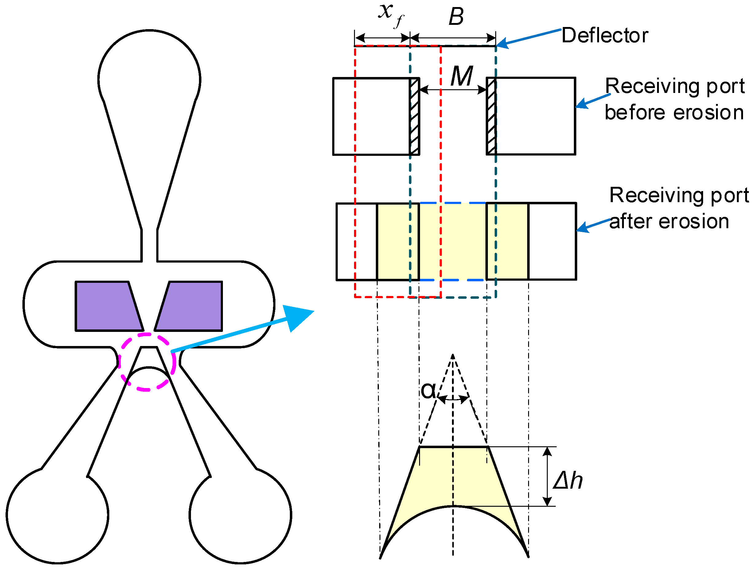
This section remodeled the flow field after erosion and researched the pressure discrepancy in both reception holes before and after erosion. As shown in Figure 14, assuming that the erosion wear height of the shunt wedge was $\Delta h$, the mass of erosion wear was $\Delta m$ and the volume of erosion wear was $\Delta V$. After the erosion, the shape of the receiving port changed in the yellow area that affected the flow between receiving holes.

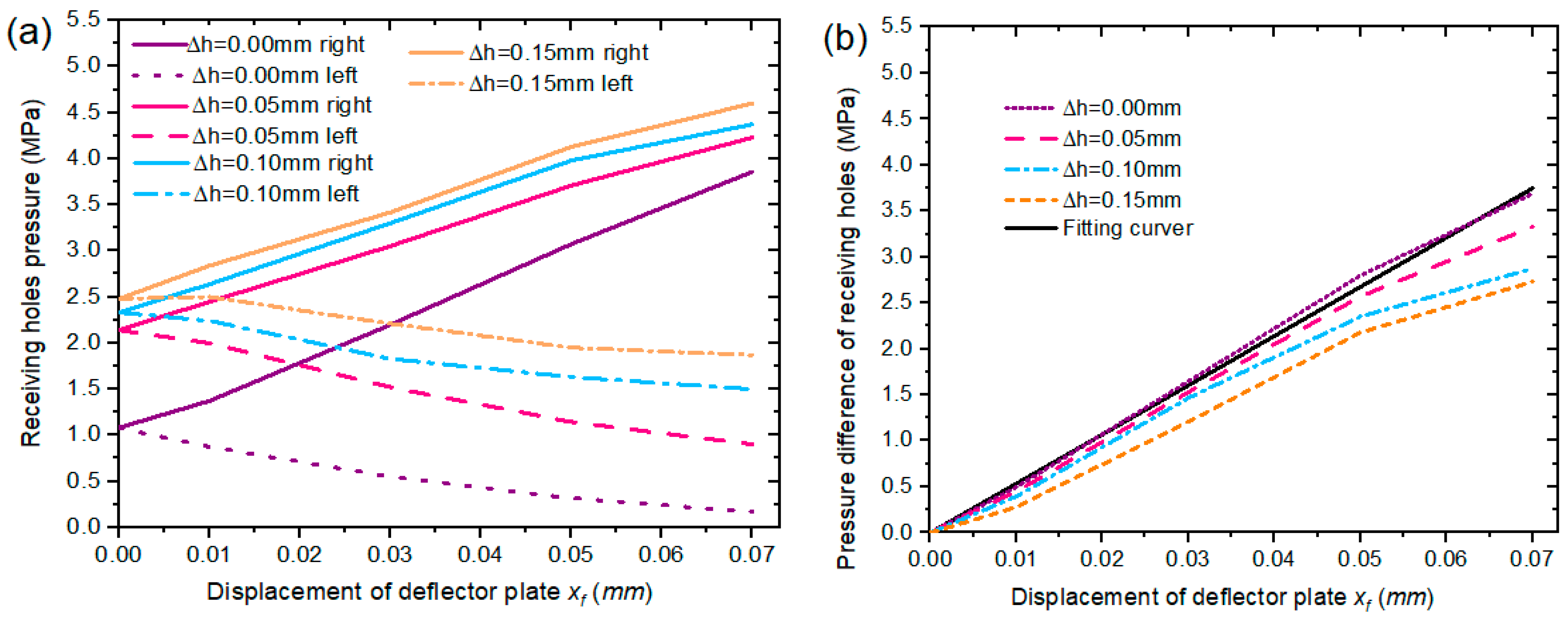
When the erosion wear height of the shunt wedge was 0.00 mm, 0.05 mm, 0.10 mm and 0.15 mm, respectively, the pressure and pressure difference of two receiving holes were shown in the Figure 15. The pressure of each receiving hole increased, but the pressure difference decreased. Especially when the erosion wear height of shunt wedge was 0.15 mm, the drop of pressure difference was quite severe. According to the working principle of the valve, the decline of pressure difference led to increasing the pushing force to the core valve, which reduced the sensitivity of the servo valve.

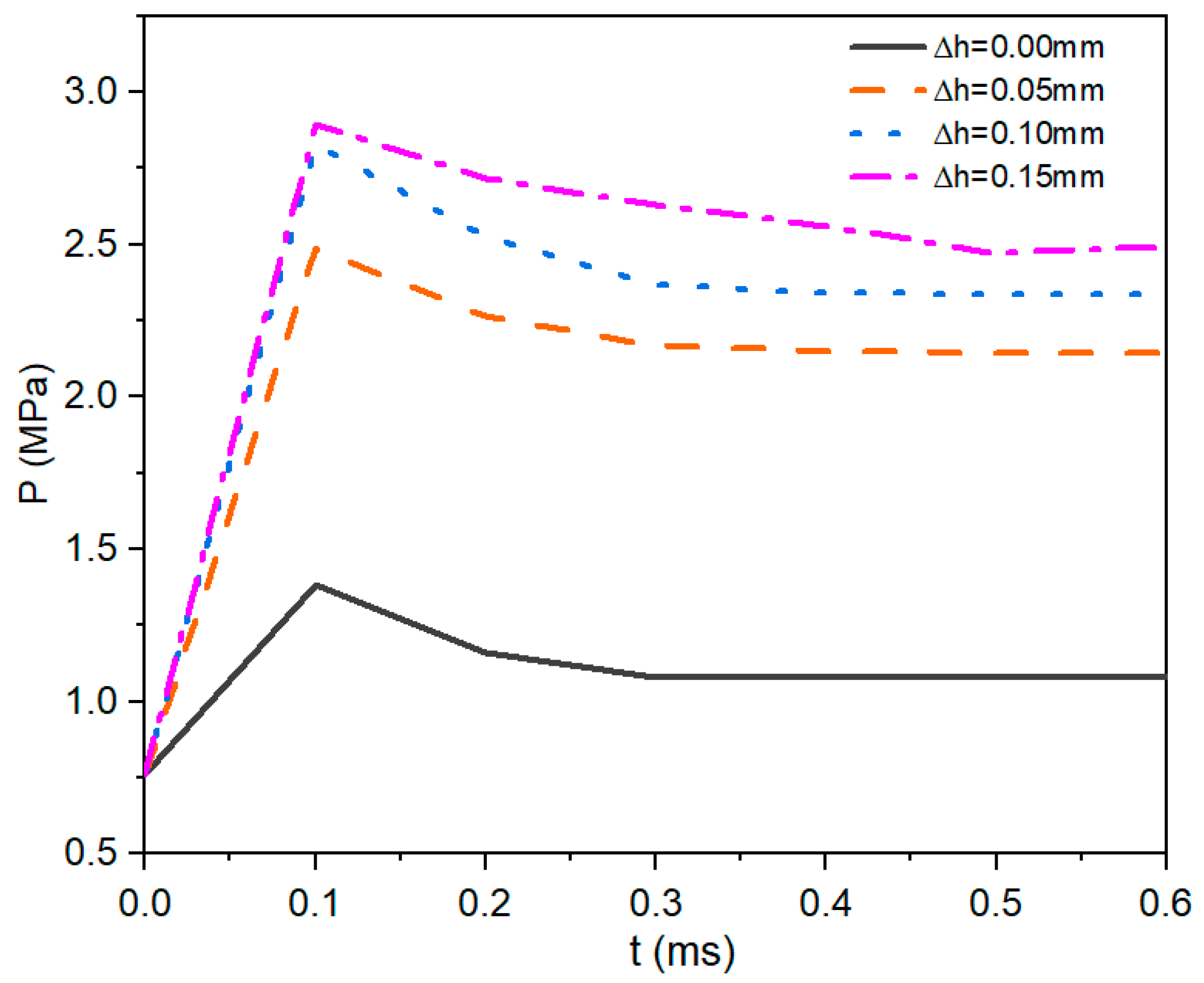
Figure 16 shows the transient pressure in receiving holes under different erosion wear height of shunt wedge. With the increase in erosion wear height, the maximum transient pressure in receiving hole gradually grew. However, it can reach the steady-state in a very short time. Even if the erosion height of shunt wedge was 0.15 mm, the transient pressure in receiving hole can reach the steady-state at 0.5 ms, which was a very fast time relative to the steady adjustment time of the whole valve. So as to, the erosion had little influence on the transient pressure of the two receiver holes.

5.5. Impact of Erosion on Valve Performance and Life Prediction

With the whole valve model deduced in Section 2.1, the valve performance was studied in MATLAB platform by the SIMULINK module. Combining the fitting coefficient $Kp$ of the pressure difference under different erosion heights, the step signal with an amplitude of 40 mA was input to simulate. Brake pressures before and after erosion were obtained, as shown in the Figure 17.

The figure showed that the braking pressure was changed significantly before and after erosion. The braking pressure gradually dropped from 21 MPa to 17.5 MPa under the same signal as the erosion height increased. This event was proposed to be mainly because, with an increase in the erosion height, the pressure difference in the valve ‘s control chamber decreased, resulting in a loss of force to move the slide valve and a reduction in valve opening. In such cases, the step signal amplitude must be increased to reach the specified brake pressure, thereby reducing the sensitivity of the valve.

Furthermore, referring to Figure 14, the relationship between the shunt wedge wear height, erosion wear rate (ER) and erosion time T can be expressed as below:

$$\Delta m=\Delta V\cdot {\rho }_W=ER\cdot \frac{\Delta V}{\Delta h}\cdot T$$

(35)

$$T=\frac{{\rho }_W}{ER}\cdot \Delta h$$

(36)

where ${\rho }_W$ is the density of the wall.

Combining the mathematical model of valve, the critical erosion height $\Delta h$ can be determined and the endurance life of pre-stage erosion wear can be calculated by Equations (35) and (36). Assuming that when the output pressure value was less than 20% of the specified brake pressure, the failure happened. Combined with MATLAB and FLUENT simulation analysis, the erosion height was 0.18 mm, the erosion life under different contamination degree was shown in Figure 18, which followed exponential distribution corresponding to the distribution of particles under different pollution levels. The erosion life was 9593 h under level of 7. Therefore, to ensure the service life of 9593 h, the cleanliness of the hydraulic oil should be maintained at least level of 7.

6. Conclusions

In summary, we present an approach for evaluating degradation in performance and predicting the erosion lifespan of the DJSV on different levels of oil pollution. First, the entire valve’s mathematical model as well as the erosion model were constructed; then, the erosion wear of the prestage was analyzed with two typical calculation models by simulating in an ANSYS environment. Next, the performance degradation of the whole valve was analyzed by combining the theoretical analysis with the erosion simulation results, followed by a final prediction of the valve’s erosion life. Consequently, the following conclusions were made:

The outcomes showed that the receiving holes’ shunt wedge had the highest erosion rate, which rose in proportion to the level of pollution. However, the growth rate was faster after level 7, owing to the oil above this level containing significantly more large-sized particles with a bigger momentum and stronger impact.

As the deflector moved, investigations revealed that the erosion area was also displaced in the same direction, causing the maximum erosion rate to increase initially and later decline; however, when the deflector displacement was 0.03 mm, the erosion rate reached the highest value, which is based on the structure and influence of the particle speed, collision frequency, and collision angle between the particle and the wall.

With an increased erosion wear height of the shunt wedge, the two receiving holes’ pressure difference decreased, and its linearity error increased, thus decreasing the force required to move the slide valve and, as a result, the sensitivity of the servo valve.

Combined with MATLAB and FLUENT simulation, the erosion life under different contamination degrees was predicted, which followed exponential distribution corresponding to the distribution of particles under different pollution levels.