Multidisciplinary Optimization and Analysis of Stratospheric Airships Powered by Solar Arrays

Abstract

Stratospheric airships have much potential in military and commercial applications. Design, analysis and optimization of stratospheric airships involves complex trade-off of different disciplines, and hence a multidisciplinary approach is essential. This paper describes a methodology coupling several disciplines and involving seven design variables to obtain the optimal design of a stratospheric airship powered by solar arrays. A numerical method is established to calculate the output power of the solar array in the optimization process. The optimal solutions are obtained using hybrid algorithms. The methodology can obtain the optimal envelope shape, solar array layout and other general configurations of subsystems. Results show that the methodology was able to achieve a solution with a 19.2% reduction in airship volume compared to the value being part of an arbitrary initial set of airship parameters. In addition, a comparative study is carried out to highlight the importance of considerations of solar array layouts and array circumferential location. Furthermore, detailed sensitivity analysis shows that operating parameters of latitudes, heading angles and average resisting wind speeds have significant effects on the airship design and solar array layouts.

1. Introduction

With potential in military and civil applications including communication, surveillance, observation and scientific research, there is a growing interest in studying stratospheric airships in recent years [1,2,3]. Stratospheric airships generally remain aloft at specific altitudes (18~22 km) for long endurance (several months) using buoyancy of lighter-than-air gas [4,5,6]. To achieve the long-endurance station-keeping task, renewable energy systems are generally used, which is mainly composed of energy-generating cells, energy-storage batteries and energy management devices [7]. Many studies have been conducted to investigate the feasibility of stratospheric solar-powered airships [8,9,10,11,12]. Generally, flexible solar arrays are placed on the surface of the airship envelope [13]. However, a design using solar arrays with higher area and mass might lead to a considerable decrease in the entire airship system mass, even though the mass fraction of energy system mass to total airship mass may increase. Therefore, a multidisciplinary optimization problem needs to be framed and solved [14].

Some previous research is focused on the performance optimization of solar array area itself. Garg et al. [15] proposed a method for optimizing the output energy of solar arrays, but considering only two design variables. More detailed optimizations for solar arrays have been conducted by Li et al. [16] and Liang et al. [17], but they are applicable only for an envelope of specific profile. Zhu et al. [18] studied the effect of layout parameters on output energy of solar array on the airship, with and without thermal effect. However, they only considered the case in which solar arrays were symmetrically placed on the upper surface of the airship.

Some studies based on multidisciplinary design optimization (MDO) were conducted, assuming the airship envelope to be an axisymmetric body of revolution. Wang et al. [19] and Michele et al. [20] have constructed an optimization framework assuming a cylindrical shaped solar array in their energy calculations, which might cause a calculation error without considering the curvature of solar array at the longitude cross-section. Alam et al. [13] established an MDO-based shape optimization method for determining the optimal envelope shape that minimizes the solar array area of a high altitude airship. Shan et al. [21] proposed a position energy storage strategy to achieve regional station-keeping by adjusting the airspeeds for flight during day and night. Ceruti et al. [22] demonstrated a shape optimization framework of hybrid airship based on added mass. Meng [23] proposed a multidisciplinary design optimization method of a lift-type hybrid airship. On the basis of building subsystem model, a Concurrent Subsystem Optimization algorithm based on Response Surface (CSSO-RS) with the self-adaptive ability is put forward. To achieve a continuous flight and reduce the total mass and energy cost, Zhang [24] proposed a multi-phase strategy including the climb, daytime cruise, glide and nighttime cruise. However, they only considered the case in which solar arrays are symmetrically located on the upper surface of airship envelope. Recently, Tang et al. [25] proposed a multidisciplinary optimization method for the semirigid stratospheric airships, but they used an empirical time-averaged solar radiation constant to predict the total power in daytime and neglected the effects of curvature of the solar array. In addition, studies focused on unconventional non-axisymmetric body of revolution such as sum of two ellipsoids [17] and multi-lobed hybrid [26,27] have also been conducted. The above research focused on a traditional design layout in which the solar array is symmetrically fixed on the upper surface of the airship envelope.

Studies indicate that the circumferential locations of the solar arrays significantly affect the electrical energy output. Lv et al. [28] found that the central angle of solar array has a significant influence on output energy. However, they focused only on solar layouts for fixed airship parameters, without considering other disciplines. Lv et al. [29] studied the advantages of cylindrical shaped solar array, without considering the coupling effects of the attitudes, latitudes, heading angles and dates on the optimal rotation angles of the solar array. In a recent study, Zhang et al. [30] established a multidisciplinary design methodology to minimize the total mass of the airship and used central angles of the solar arrays as design variables. However, the common shortcoming of the above studies is that the calculation formulation of required storage battery capacity considered only the time discharged at night, without considering the simultaneous operation of battery and solar array when the output power of solar array is lower than required power in daytime.

In general, existing methodologies for designing stratospheric airships powered by solar arrays either assume a fixed envelope, or only consider the case in which the solar array is symmetrically located on the upper surface of airship envelope or adopt simple energy balance models. This simplification makes it difficult to obtain the solar cell layout with high power generation efficiency. Therefore, improved optimization methodologies for designing stratospheric airship powered by solar arrays are required.

This study proposes an optimization methodology for searching for the optimal layouts including the central angle of solar array on airship envelope, considering the trade-offs among different disciplines and critical constraints of energy balance and buoyancy equilibrium. The proposed methodology can optimize the stratospheric airship configurations by considering the envelope shape, the solar array layouts, etc., using detailed subsystem models. Based on the proposed method, an optimization case on a baseline airship model is conducted and discussed. Furthermore, the effects on the airship design of latitudes, heading angles and average resisting wind speeds are studied in detail. The rest of the paper is organized in four parts, viz., Theory, Optimization Method, Results and Discussions, and Conclusions. Figure 1 shows the research plan of the paper.

2. Theory

This section is divided into four parts. The first is the airship geometry model. The second is the output power model of solar array, including the solar radiation model, position calculation model of the sun and the numerical calculation model of output power model for curved solar arrays. Then, the energy balance model and buoyancy balance model are established.

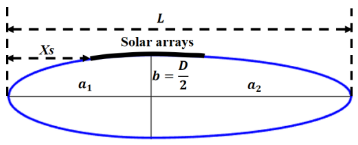
2.1. Airship Geometry Model

The streamlined stratospheric airship envelope approximately consists of two semi-spheroids (Figure 2); the volume and surface area of the envelope of the airship can be calculated as follows:

$$V_{env}=\frac{2}{3}\pi \left(a_1+a_2\right)b^2=\frac{\pi L{D}^2}{6},$$

(1)

$$S_{env}=2\pi \left(a_1+a_2\right)b=\pi LD,$$

(2)

where $L=a_1+a_2$ is the airship length, and $D=2b$ is the airship diameter.

Generally, the volume $V_{env}$ and surface of an airship $S_{env}$ can be estimated as follows:

$$V_{env}=\frac{K_V}{{(L/D)}^2}{L}^3,$$

(3)

$$S_{env}=\frac{K_s}{\left(L/D\right)}{L}^2.$$

(4)

Considering the streamlined form of the airship tail, $K_V$ and $K_S$ can be selected to be 0.5212 and 2.547 [31], respectively. The fineness ratio of airship is defined as

$$f_r=\frac{L}{D}=\frac{a_1+a_2}{2b}.$$

(5)

2.2. Output Power Model of Solar Array

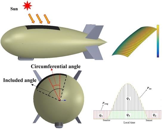
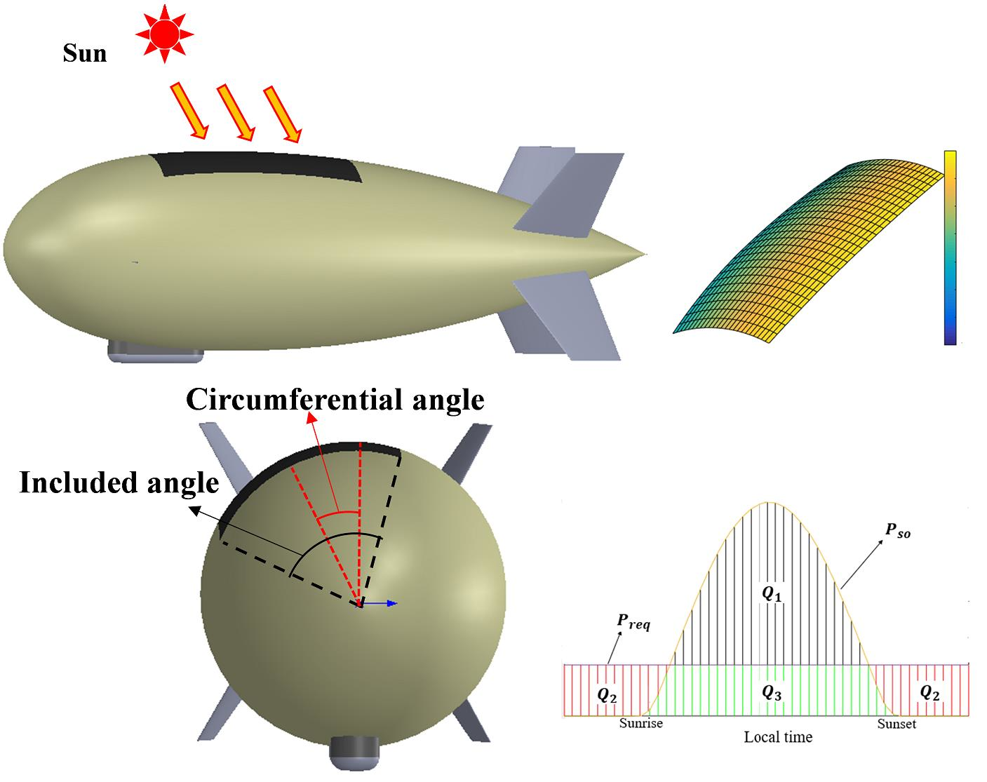
2.2.1. Solar Radiation Flux Model

Solar radiation flux can be written as [32]

$$I={\tau }_{atm}{I}_{\mathrm{sun}},$$

(6)

where ${\tau }_{atm}$ is atmospheric transmittance, which can be estimated using the formula suggested by Farley [33] as

$${\tau }_{atm}=0.5\exp \left(-0.65m_{ar}\right)+\exp \left(-0.095m_{ar}\right),$$

(7)

where $m_{ar}$ is air mass ratio when sunlight passes through the atmosphere, which can be described as

$$m_{ar}=\left\{\begin{array}{c}\left(\frac{p_a}{p_0}\right)\left[\sqrt{1229+{\left[614sin\left(h\right)\right]}^2}-614sin\left(h\right)\right]\hspace{0.33em}\hspace{0.33em}\hspace{0.33em}\hspace{0.33em}\hspace{0.33em}\hspace{0.33em}\hspace{0.33em}\hspace{0.33em}\hspace{0.33em}\hspace{0.33em}\hspace{0.33em}\hspace{0.33em}\hspace{0.33em}\hspace{0.33em}\hspace{0.33em}\hspace{0.33em}\hspace{0.33em}\hspace{0.33em}\hspace{0.33em}0 < h<\pi \\ \left(\frac{p_a}{p_0}\right)\left(1+\frac{h}{{cos}^{-1}\left(\frac{H}{H+R_{ear}}\right)}\right)-\frac{70h}{{cos}^{-1}\left(\frac{H}{H+R_{ear}}\right)}\hspace{0.33em}\hspace{0.33em}\hspace{0.33em}\hspace{0.33em}\hspace{0.33em}\hspace{0.33em}\hspace{0.33em}\hspace{0.33em}\hspace{0.33em}\hspace{0.33em}\hspace{0.33em}\hspace{0.33em}h \le 0\hspace{0.33em}or\hspace{0.33em}h \ge \pi \end{array}\right.$$

(8)

where $p_a$ is atmosphere pressure at the flight altitude, and $p_0$ is the standard atmosphere pressure at sea level. $R_{ear}$ is the radius of the earth which is generally set to be 6,400,000 m (6400 km), $H$ is the flight altitude.

Figure 3 shows a sketch of the position of the sun. As shown in the figure, $h$ is the sun elevation angle, which can be expressed as [34]

$$h={sin}^{-1}\left(sin \delta sin \varphi + cos \delta cos \omega cos \varphi \right),$$

(9)

where $\delta$ is the declination angle of the sun, $\varphi$ is the latitude of flight and $\omega$ is the hour angle of the sun.

The solar radiation flux of the exoatmosphere $I_{\mathrm{sun}}$ can be calculated with the approximate formula [35]

$$\left\{\begin{array}{l}{I}_{sun}=I_0\left\{1+0.5\left[{\left(\frac{1+e}{1-e}\right)}^2-1\right]cos\left(TA\right)\right\}\\ TA=2\pi \frac{n-2}{n_p}\end{array}\right.,$$

(10)

where $I_0$ is the solar radiation intensity constant which has a value of 1367 W/m², e = 0.016708 is the eccentricity of earth’s orbit, $n$ is the day number starting from perihelion, and $n_p$ is the total number of days of the year.

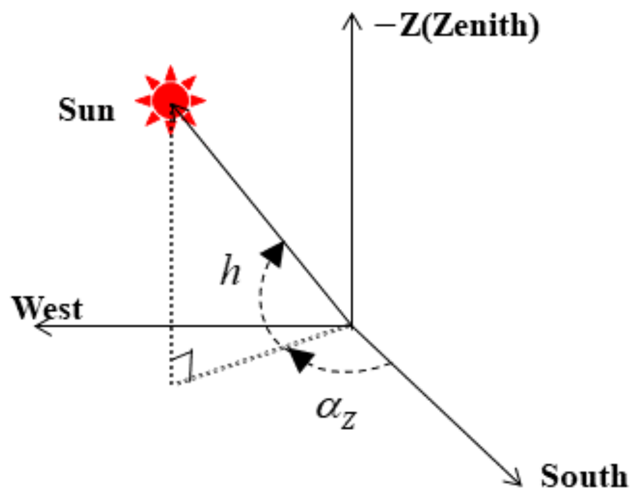
2.2.2. Position of the Sun

As shown in Figure 3, the position vector of the sun can be expressed as [34]

$${\overrightarrow{S}}_g={\left[-cos\hspace{0.33em}h\hspace{0.33em}cos{\alpha }_z,-cos\hspace{0.33em}h\hspace{0.33em}sin{\alpha }_z,-sin\hspace{0.33em}h\right]}^T,$$

(11)

where ${\alpha }_z$ is the sun azimuth angle.

$${\alpha }_z=sign(\omega ){cos}^{-1}\left(\frac{sin\hspace{0.33em}h\hspace{0.33em}sin\hspace{0.33em}\varphi -sin\delta }{cos\hspace{0.33em}hcos\hspace{0.33em}\varphi }\right);$$

(12)

$\delta$ can be calculated by the approximate formula [36]

$$\begin{gathered} \delta =0.3723+23.2567sin\left(\beta \right)+0.1149 sin\left(2\beta \right) - 0.1712sin\left(3\beta \right) \\ - 0.758cos\left(\beta \right)+0.3656cos\left(2\beta \right) +0.0201cos\left(3\beta \right); \end{gathered}$$

(13)

$\beta$ is the day angle of sun, which can be calculated by the following formula:

$$\left\{\begin{array}{c}\beta =\frac{2\pi \left(n-1-n_0\right)}{365.2422}\hfill \\ n_0=78.801+0.242\left(y_{ear}-1969\right)-floor \left[ 0.25\left(y_{ear}-1969\right) \right]\end{array}\right.,$$

(14)

where $y_{ear}$ is the year, $n$ is the count of days from 1 January, $floor\left[\right]$ indicates the truncation function extracting the integral part of a number.

The hour angle of sun $\omega$ can be expressed as

$$\omega =\left\{\begin{array}{c}{\lambda }_t-2\pi \hspace{0.33em}\hspace{0.33em}\hspace{0.33em}\hspace{0.33em}{\lambda }_t>\pi \hspace{0.33em}\hspace{0.33em}\hfill \\ {\lambda }_t\hspace{0.33em}\hspace{0.33em}\hspace{0.33em}\hspace{0.33em}\hspace{0.33em}\hspace{0.33em}\hspace{0.33em}\hspace{0.33em}-\pi \le {\lambda }_t\le \pi \hfill \\ {\lambda }_t\hspace{0.33em}+2\pi \hspace{0.33em}\hspace{0.33em}\hspace{0.33em}{\lambda }_t<-\pi \hspace{0.33em}\hspace{0.33em}\hfill \end{array},\right.\hspace{0.33em}\hspace{0.33em}$$

(15)

where

$${\lambda }_t=\frac{\pi \left[15(t_s+e_t-12)+\left(\lambda -{\lambda }_0\right)\right]}{180},$$

(16)

where $t_s$ is the local mean solar time, $\lambda$ is the local longitude and ${\lambda }_0$ is the reference longitude for the local time zone, and $e_t$ is the time difference between actual solar time and mean solar time which can be written as

$$e_t=\frac{9.87sin\left(2\delta \right) - 7.53cos\hspace{0.33em}\delta - 1.5sin\hspace{0.33em}\delta }{60}.$$

(17)

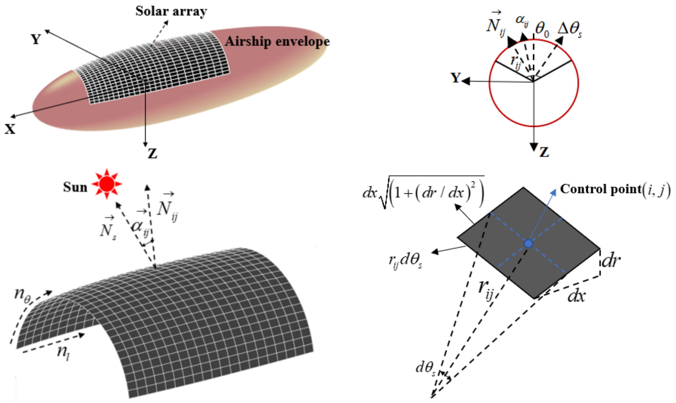
2.2.3. Output Power Model of Solar Array

Figure 4 shows the sketch of the body–axis coordinate system and the solar array cell. The stabilizers are located at the tail of airship, and their design is such that they never cast a shadow over the solar panel. The solar array is curved, and its curvature is consistent with that of the airship. It is assumed that the array consists of many micro-modules, which are assumed to be planes. The solar panels are supposed to operate at a nominal temperature, hence the impact of the temperature has not been included here. As shown in the figure, $r_{ij}$ is the circumferential radius of the element, $\overrightarrow{N_{ij}}$ is the normal vector of the element surface, $\Delta {\theta }_s$ is the total included angle of the solar array. The array is divided into $n_l$ (along with length) × $n_{\theta }$ (along with circumference).

The local circumference radius of the airship is the function of $x$, which can be expressed as

$$r=f\left(x\right)\hspace{0.33em}\hspace{0.33em}\hspace{0.33em}-a_2\le x\le a_1.$$

(18)

Then, the geometry of airship can be expressed as

$$y^2+z^2=f^2\left(x\right)\hspace{0.33em}\hspace{0.33em}\hspace{0.33em}-a_2\le x\le a_1.$$

(19)

The shape governing equation of the airship can be written as

$$F\left(x,y,z\right)=y^2+z^2-f^2\left(x\right)\hspace{0.33em}\hspace{0.33em}\hspace{0.33em}-a_2\le x\le a_1.$$

(20)

Therefore, the normal vector of element $\left(i,j\right)$ can be expressed as

$$\overrightarrow{N_{ij}}=\left(N_{ijx},N_{ijy},N_{ijz}\right)=\frac{\left(\frac{\partial F}{\partial x_{ij}},\frac{\partial F}{\partial y_{ij}},\frac{\partial F}{\partial z_{ij}}\right)}{\sqrt{{\left(\frac{\partial F}{\partial x_{ij}}\right)}^2+{\left(\frac{\partial F}{\partial y_{ij}}\right)}^2+{\left(\frac{\partial F}{\partial z_{ij}}\right)}^2}}.$$

(21)

$\overrightarrow{N_s}$ is the position vector of the sun in the body coordinate system, ${\alpha }_{ij}$ is the setting angle of the element. The transformation matrix from the inertial coordinate system to body coordinate system can be written as

$$T_{ib}=\left[\begin{array}{l}\hspace{0.33em}\hspace{0.33em}\hspace{0.33em}\hspace{0.33em}\hspace{0.33em}\hspace{0.33em}\hspace{0.33em}\hspace{0.33em}\hspace{0.33em}\hspace{0.33em}cos\left(\psi \right)\hspace{0.33em}cos\hspace{0.33em}\left(\theta \right)\hspace{0.33em}\hspace{0.33em}\hspace{0.33em}\hspace{0.33em}\hspace{0.33em}\hspace{0.33em}\hspace{0.33em}\hspace{0.33em}\hspace{0.33em}\hspace{0.33em}\hspace{0.33em}\hspace{0.33em}\hspace{0.33em}\hspace{0.33em}\hspace{0.33em}\hspace{0.33em}\hspace{0.33em}\hspace{0.33em}\hspace{0.33em}\hspace{0.33em}\hspace{0.33em}\hspace{0.33em}\hspace{0.33em}sin\left(\psi \right)cos\left(\theta \right)\hspace{0.33em}\hspace{0.33em}\hspace{0.33em}\hspace{0.33em}\hspace{0.33em}\hspace{0.33em}\hspace{0.33em}\hspace{0.33em}\hspace{0.33em}\hspace{0.33em}\hspace{0.33em}\hspace{0.33em}-sin\left(\theta \right)\\ cos\left(\psi \right)sin\left(\theta \right)sin\left(\phi \right)-sin\left(\psi \right)cos\left(\phi \right) \hspace{0.33em}\hspace{0.33em}sin\left(\psi \right)sin\left(\theta \right)sin\left(\phi \right)+cos\left(\psi \right)cos\left(\phi \right)\hspace{0.33em}\hspace{0.33em}cos\left(\theta \right)sin\left(\phi \right)\\ cos\left(\psi \right)sin\left(\theta \right)cos\left(\phi \right)+sin\left(\psi \right)sin\left(\phi \right)\hspace{0.33em}\hspace{0.33em}\hspace{0.33em}sin\left(\psi \right)sin\left(\theta \right)cos\left(\phi \right)-cos\left(\psi \right)sin\left(\phi \right) \hspace{0.33em}cos\left(\theta \right)cos\left(\phi \right)\end{array}\right],$$

(22)

where $\psi$ is the heading angle of airship, $\theta$ is the pitch angle, $\phi$ is the roll angle. Generally, $\theta$ and $\phi$ are very small and thus can be assumed to be zero. The position vector of sun in the body coordinate system can be written as

$$\overrightarrow{N_s}=\left(N_{sx},N_{sy},\hspace{0.33em}{N}_{sz}\hspace{0.33em}\right)=T_{ib}\overrightarrow{S_g}.$$

(23)

The angle between the sun position vector and the element normal vector can be expressed as

$${\alpha }_{ij}{=cos}^{-1}\left(\frac{{\overrightarrow{N}}_{ij}{\overrightarrow{S}}_g}{\left|{\overrightarrow{N}}_{ij}\right|\left|{\overrightarrow{S}}_g\right|}\right).$$

(24)

The solar panels are supposed to operate at a nominal temperature, hence the impact of the temperature has not been included. The power received by element $\left(i,j\right)$ can be expressed as

$$P_{ij}=\left\{\begin{array}{c}I{s}_{ij}cos\left({\alpha }_{ij}\right)\hspace{0.33em}\hspace{0.33em}\hspace{0.33em}0\le {\alpha }_{ij}<\frac{\pi }{2}\hfill \\ 0\hspace{0.33em}\hspace{0.33em}\hspace{0.33em}\hspace{0.33em}\hspace{0.33em}\hspace{0.33em}\hspace{0.33em}\hspace{0.33em}\hspace{0.33em}\hspace{0.33em}\hspace{0.33em}\hspace{0.33em}\hspace{0.33em}\frac{\pi }{2}\le {\alpha }_{ij}\le \pi \hfill \end{array}\right..$$

(25)

In the above equation, $\frac{\pi }{2}\le {\alpha }_{ij}\le \pi$ means the element is shadowed, and no radiation will be received by the element. Therefore, the element will not produce any power at this condition. $s_{ij}$ is the surface area of the element $\left(i,j\right)$, as shown in the figure; it can be calculated as follows:

$$s_{ij}=r_{ij}d{\theta }_{s}dx\sqrt{\left(1+{\left(\frac{dr}{dx}\right)}^2\right)}.$$

(26)

Therefore, the total output power of the solar array at a certain time can be expressed as

$$P_{so}\left(t\right)={\eta }_{so}\sum _{i=1}^{n_{\theta }}\sum _{j=1}^{n_l}{P}_{ij}\left(t\right),$$

(27)

where ${\eta }_{so}$ is the transformation efficiency of the solar cell, $P_{ij}$ is the output power of the element $\left(i,j\right)$.

The total area of solar arrays can be calculated as

$$S_{so}={{\displaystyle \int }}_{x_s}^{x_e}{{\displaystyle \int }}_{{\theta }_0-\frac{\Delta \theta }{2}}^{{\theta }_0+\frac{\Delta \theta }{2}}r\left(x\right)\sqrt{\left(1+{\left(\frac{dr}{dx}\right)}^2\right)}d{\theta }_{s}dx,$$

(28)

where $x_s$ and $x_e$ are the coordinates of leading edge and trailing edge of solar array, ${\theta }_0$ is the central angle of solar array and $\Delta \theta$ is the included angle of solar array.

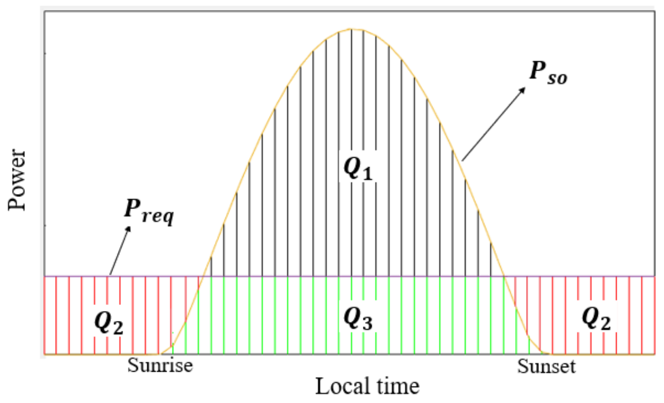
2.3. Energy Balance Model

The total power required for an airship ($P_{req}$) mainly consists of power consumed by propulsion subsystem ($P_{prp}$), control system ($P_{ctr}$) and payload ($P_{pay}$), which can be described as

$$P_{req}=P_{prp}+P_{ctr}+P_{pay},$$

(29)

where $P_{ctr}$ and $P_{pay}$ are generally assumed to be constant, and $P_{prp}$ can be calculated as

$$P_{prp}=\frac{1}{2}{\rho }_a{V}_0^3{C}_D{V}_{env}^{2/3}{\eta }_{prp},$$

(30)

where $V_0$ is the average flight speed of airship, and ${\eta }_{prp}$ is the efficiency of propulsion subsystem. $C_D$ is the drag coefficient of airship, $V_{env}^{2/3}$ is the reference area of airship. Hoerner proposed the following empirical formula to estimate the drag of streamline bodies of revolution in turbulent flow at zero angle of attack [37,38]:

$$C_{D0}=\frac{0.18f_r{}^{1/3}+0.27f_r{}^{\left(-7/8\right)}+1.08f_r{}^{\left(-8/3\right)}}{R_e{}^{1/6}},$$

(31)

where $f_r$ is the fineness ratio of airship defined by Equation (5), and $R_e$ is the Reynolds number and can be written as

$$R_e=\frac{{\rho }_a{V}_{0}L}{\mu },$$

(32)

where $\mu$ is the dynamic viscosity of ambient air, and ${\rho }_a$ is the local air density which can be calculated using the following formula [39]:

$${\rho }_a\left(H\right)=\left\{\begin{array}{c}1.225{\left(\frac{288.15-0.0065H}{288.15}\right)}^{4.2559} H\le 11000 \mathrm{m}\hfill \\ 0.3639e^{\left(-\frac{H-11000}{6341.62}\right)} 11000\le H\le 20000 m \hfill \end{array}\right. .$$

(33)

The units of above constants are as follows: 1.225-kg/m³, 288.15-K, 0.0065-K/m, 11,000-m, 6341.62-m. $C_D$ can be calculated as

$$C_D=\Gamma C_{D0}.$$

(34)

$\Gamma$ is an empirical parameter considering the aerodynamics effects of other components on the airship, which is set to be 1.8 in this study.

Figure 5 shows a sketch map for illustration of the energy balance. As shown in the figure, $Q_3$ is the energy generated by solar arrays which is directly used for running the airship, $Q_1$ is the available surplus energy for storage in lithium battery when $P_{so}>P_{req}$, $Q_2$ is the energy consumption, which needs to be supplied by the lithium battery. Obviously, the total energy generated by the solar array in daytime should not be less than the required energy of the airship over one day. Therefore, the energy balance model can be described as

$$Q_1{\eta }_{lic}{\eta }_{lid}+Q_3\ge Q_{req},$$

(35)

where ${\eta }_{lic}$ and ${\eta }_{lid}$ are the charge efficiency and discharge efficiency of lithium battery, respectively. $Q_1$, $Q_3$ and $Q_{req}$ can be calculated as

$$Q_1={\displaystyle {\int }_{T_0}^T{U}_{\left(P_{so}-P_{req}\right)}\left[P_{so}\left(t\right)-P_{req}\left(t\right)\right]}dt,$$

(36)

$$Q_3={\displaystyle {\int }_{T_0}^T{P}_{so}\left(t\right)dt-Q_1},$$

(37)

$$Q_{req}={\displaystyle {\int }_{T_0}^T{P}_{req}\left(t\right)dt},$$

(38)

where $U_{\left(\right)}$ is the unit step function, and its value is 1 when $P_{so}>P_{req}$ while it is 0 for $P_{so}\le P_{req}$.

2.4. Buoyancy Balance Model

At flight altitude ($H$), the buoyancy of airship ($F_b$) is required not to be less than the total weight, which can be described as

$$f_{bm}\left(H\right)=F_b\left(H\right)-m_t\mathrm{g}\ge 0 ,$$

(39)

where $F_b$ can be calculated as

$$F_b={\rho }_a{V}_{env}g.$$

(40)

The total mass of airship ($m_t$) can be expressed as

$$m_t=m_{str}+m_{ene}+m_{prp}+m_{pay}+m_{oth},$$

(41)

where $m_{str}$ is the total mass of structural subsystem, $m_{ene}$ is the total mass of energy subsystem, $m_{prp}$ is the mass of propulsion subsystem, $m_{pay}$ is the mass of payload, $m_{oth}$ is the mass of other components.

Total mass of structural subsystem $m_{str}$ can be calculated as

$$m_{str}=m_{env}+m_{fin}+m_{gas},$$

(42)

where $m_{env}$, $m_{fin}$ and $m_{gas}$ are the mass of the airship envelope, mass of the fin and mass of the gas in the airship [14], respectively. $m_{env}$ can be calculated as

$$m_{env}=1.25{\rho }_{env}{S}_{env},$$

(43)

where ${\rho }_{env}$ is the areal density of envelope, and the coefficient 1.25 is a factor considering the attachments on the envelope.

The mass of the fin can be calculated as

$$m_{fin}=1.25{\rho }_{fin}{S}_{fin},$$

(44)

where ${\rho }_{fin}$ is the areal density of the fin. The surface area of the fin $S_{fin}$ can be estimated using the empirical equation

$$S_{fin}=0.0121V_{env}.$$

(45)

The mass of the gas in the airship can be calculated as

$$m_{gas}={\rho }_a{V}_{env}{n}_{ga},$$

(46)

where $n_{ga}$ is the ratio of molecular mass of gas to that of air.

$m_{ene}$ is the sum of mass of solar array ($m_{so}$) and lithium battery ($m_{li}$), which can be expressed as

$$m_{ene}=m_{so}+m_{li},$$

(47)

where

$$m_{so}={\rho }_{so}{S}_{so},$$

(48)

$$m_{li}=\frac{\left(Q_{req}-Q_3\right)}{{\eta }_{lid}{\delta }_{li}},$$

(49)

where ${\rho }_{so}$ is the aerial density of solar array and ${\delta }_{li}$ is the energy density of battery.

$m_{prp}$ can be expressed as

$$m_{prp}=\frac{P_{prpmax}}{{\delta }_{pm}},$$

(50)

where ${\delta }_{pm}$ is the power density of the propulsion subsystem. $P_{prp\max }$ is the required power of the propulsion subsystem for the maximum designed flight speed of the airship.

Finally, mass of other components on the airship ($m_{oth}$) can be estimated as [40]

$$m_{oth}=0.25\left(m_{ene}+m_{env}+m_{fin}+m_{prp}\right).$$

(51)

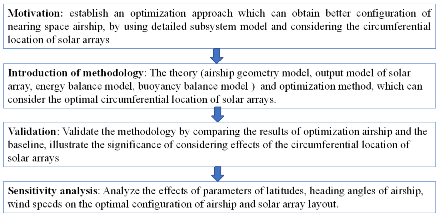
3. Optimization Method

This paper mainly proposes an approach which can optimize the solar array layout and the general parameters of the airship. By conducting the optimization cases, we validate that the total mass or size can be further reduced with consideration of the circumferential location of the solar array. Then, in the sensitivity analysis, all parameters are optimized including the circumferential location of the solar array.

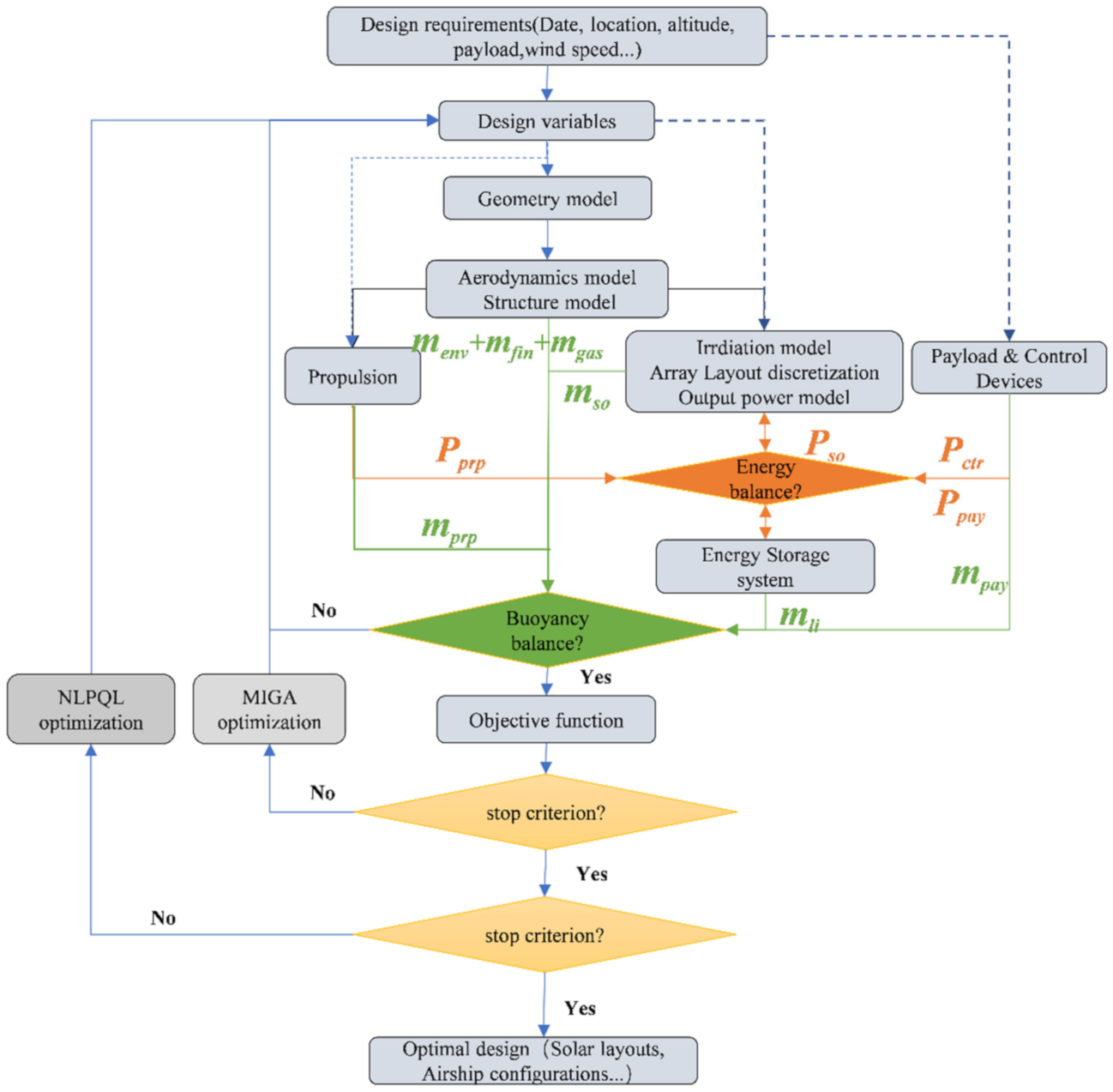
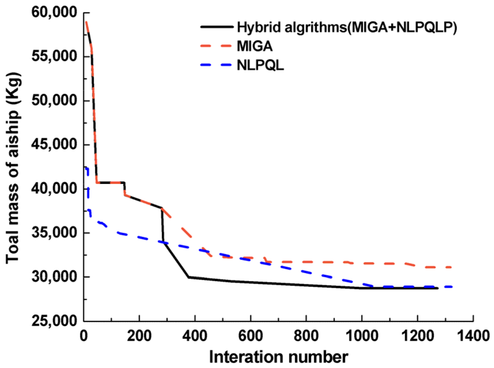
3.1. Optimization Methodology

Generally, optimization methods fall into the categories of non-gradient-based algorithms, gradient-based algorithms, and hybrid algorithms. The non-gradient-based algorithms can obtain the global optimum (optimum in the whole design space) without calculating the local gradient and strict requirement of the start point. However, they are generally inefficient. Gradient-based algorithms are efficient, but they obtain the local optimum (optimum in certain local space) with ease; they highly rely on the start searching points to obtain the global optimum. The hybrid algorithms, which combine the good overall domain exploration properties of the non-gradient-based algorithm with the fast convergence properties of the gradient-based algorithm, can generally obtain the optimum solution efficiently and reliably. Therefore, the hybrid algorithms are adopted in this study. Firstly, MIGA (Multi-Island Genetic Algorithm) [41] is applied to obtain an initial global optimization solution. Then, NLPQL (Nonlinear Programming by Quadratic Lagrangian) [42] is executed starting with this solution to further determine the optimum solution.

MIGA is developed based on the Genetic Algorithm (GA). Each population of individuals is divided into several sub-populations called “Islands”. By evaluating the fitness of each individual, a set of individuals which best adapts to the natural environment is selected in each generation. These individuals are subsequently sent to the next generation with crossover and mutation under certain probability. This process is repeated until the convergence criterion is satisfied. NLPQL is a sequential quadratic programming method. A linearization of the constraints and a quadratic approximation of the Lagrangian function are used in the algorithm. To generate a search direction, a quadratic sub-problem is formulated and solved. The line search can be performed with respect to two alternative merit functions, and the Hessian approximation is updated using a given formula. Figure 6 shows the flowchart of optimization process for stratospheric airship proposed in this study. The main steps are as follows:

Step 1: Define the design requirements.

Step 2: Define the design variables.

Step 3: Generate the geometry model.

Step 4: Using the aerodynamics model, structure model to calculate the aerodynamics of airship and mass of subsystems.

Step 5: Calculate the required propulsion power and energy, and calculate the mass of propulsion subsystem and energy subsystem.

Step 6: Estimate the buoyancy balance; if it is satisfied, proceed to next step; otherwise, proceed to Step 2 and change the value of design variables.

Step 7: Estimate the objective function; if the stop criterion of MIGA optimization is satisfied, then proceed to next step, otherwise proceed to Step 2.

Step 8: Conduct the NLPQL optimizations until the stop criterion is satisfied.

Step 9: Output the optimization results.

3.2. Variables and Constants

Table 1. Design variables and design space.

Full Name of Parameters	Parameter	Lower Bound	Upper Bound
Semimajor axis of the front part of airship (m)	$a_1$	50	150
Semimajor axis of the rear part of airship (m)	$a_2$	50	150
Fineness ratio of airship	$f_r$	3	5
Horizontal distance from the airship nose to the front of solar arrays (m)	$x_s$	20	100
Horizontal distance from the airship nose to the rear of solar arrays (m)	$x_e$	50.0	200.0
Included angle of solar arrays ($°$)	$\Delta {\theta }_s$	60	180
Central angle of solar arrays ($°$)	${\theta }_0$	−30.0	90

lists the design variables and corresponding bounds on their upper and lower values. Seven parameters are considered, which are related to the layout of solar array and the shape of the airship envelope.

Table 2. Parameter values used for the airship problem.

Full Name of Parameters	Parameter	Value
Transformation efficiency of the solar cell (%)	${\eta }_{so}$	18
Efficiency of propulsion subsystem (%)	${\eta }_{prp}$	55
Charge efficiency of lithium battery (%)	${\eta }_{lic}$	95
Discharge efficiency of lithium battery (%)	${\eta }_{lid}$	98
Areal density of solar arrays (kg/m2)	${\rho }_{so}$	0.65
Areal density of envelope (kg/m2)	${\rho }_{env}$	0.125
Areal density of fin (kg/m2)	${\rho }_{fin}$	0.06
Energy density of battery (Wh/kg)	${\delta }_{li}$	200
Power density of propulsion subsystem (W/kg)	${\delta }_{prp}$	222
Power consumed by control system (W)	$P_{ctr}$	1000
Power consumed by payload (W)	$P_{pay}$	5000
Mass of payload (kg)	$m_{pay}$	500
Average flight speed of airship (m/s)	$V_0$	25
Maximum flight speed of airship (m/s)	$V_{\max }$	30

shows the values of parameters used in the models and equations presented in Section 2 of this paper; these values allow calculation of responses used in the objective function and constraints for the airship problem.

3.3. Objective Function and Constraints

In the present study, the goal is to minimize the total weight of the airship powered by the solar array layouts subject to the power balance constraint and to the buoyancy constraint. Therefore, the objective function and constraints can be written as

$$\begin{array}{l}min:\hspace{0.33em}f\left(X\right)=m_{tot}\\ s.t.\hspace{0.33em}\hspace{0.33em}{Q}_1{\eta }_{lis}{\eta }_{lio}+Q_3-Q_{req}\ge 0\\ \hspace{0.33em}\hspace{0.33em}\hspace{0.33em}\hspace{0.33em}\hspace{0.33em}{F}_b-m_{tot}\mathrm{g}\ge 0\end{array}$$

(52)

where X is the design variables.

4. Results and Discussions

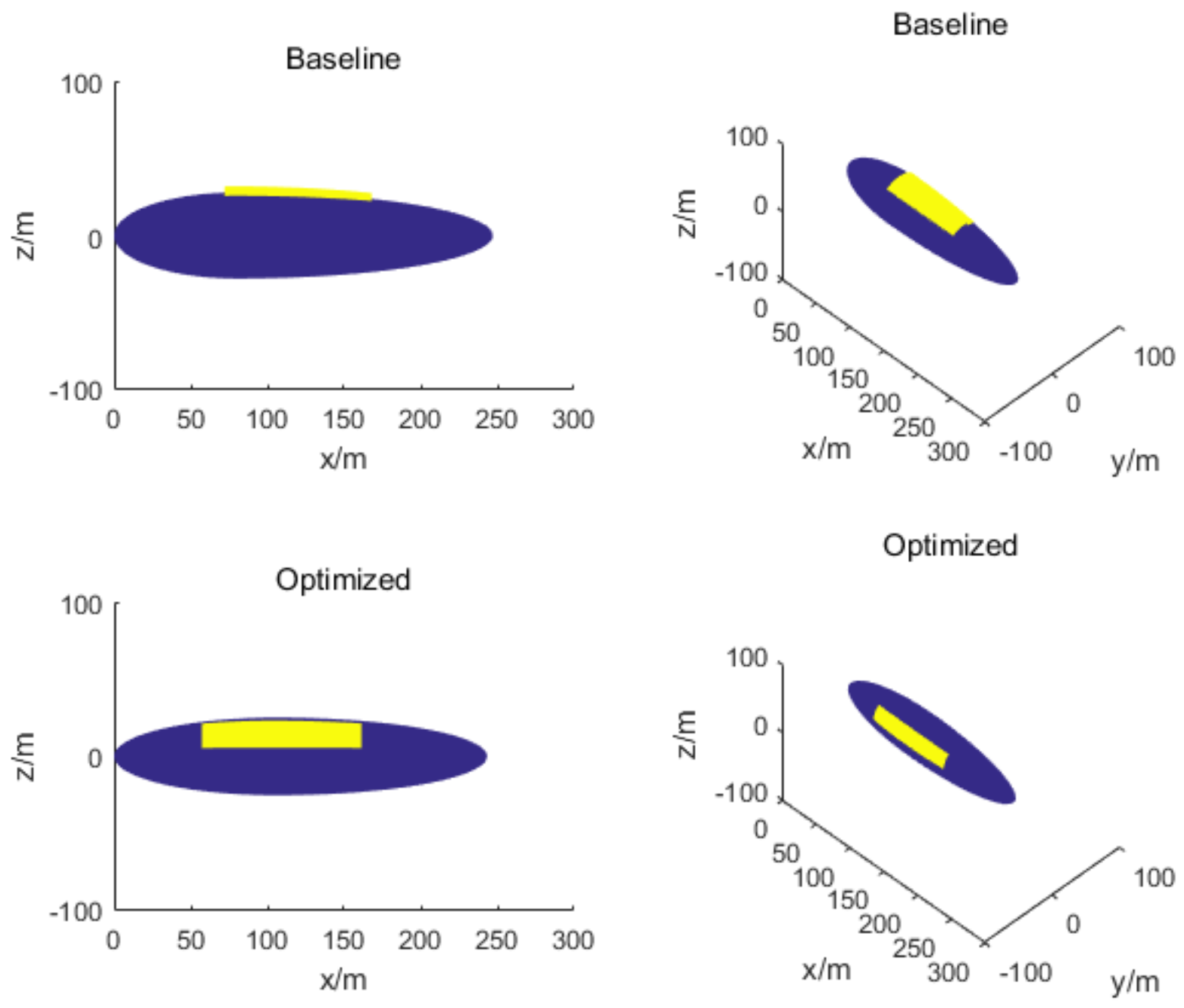
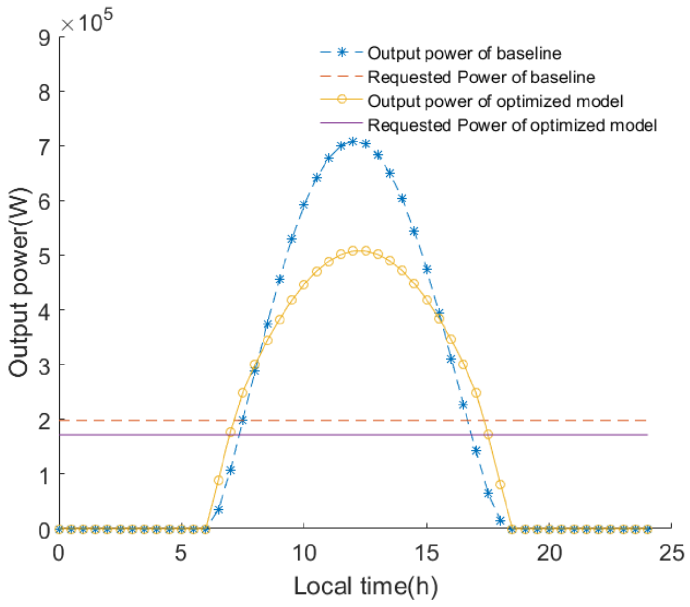
4.1. Optimization on the Baseline Model

Figure 7 shows the comparison of optimization convergence history using hybrid algorithm, MIGA and NLPQL. In the MIGA optimization, the sub-population size, number of islands, and number of generations are all set to be 10, while in the NLPQL optimization, the number of max iterations is set to be 150. It can be observed that the hybrid algorithm is of the best convergence and retrieval efficiency.

Table 3. Comparisons of key configuration parameters of baseline and optimized airship.

Parameter	Arbitrary Baseline	Optimized	Relative Difference (%)
Volume of airship (m3)	405,690	325,257	−19.83
Length of airship (m)	247	243.3	−1.5
Fineness ratio	4.40	4.80	9.19
Mass of solar array (kg)	2669.4	1507.9	−43.51
Mass of storage (kg)	14,222	11,389	−19.91
Total mass of energy system (kg)	16,891	12,897	−23.65
Total mass of airship (kg)	35,708	28,629	−19.82
Requested averaged power (kW)	198	171	−13.63
Area of solar array (m3)	4106.8	2319.7	−43.51
Central angle of solar array ($°$)	0.0	295.7	-
Included angle of solar array ($°$)	87.75	50.06	-
Start of solar array (m)	70	55.08	-
Horizontal projection length of solar array (m)	100	108.46	-

shows comparisons of key parameters between an arbitrary baseline airship (used as initial parameter set) and an optimized model. Both models are designed meeting the same operating conditions. The altitude, longitude and latitude are 20 km, ${108}^{°}$ E and ${18}^{°}$ N, respectively. The heading angle is 90° (flying from west to east). Mass of payload, power of payload, average resisting wind speed and maximum resisting wind speed are 500 kg, 5000 W, 25 m/s and 30 m/s, respectively.

As shown in the table, the volume and length of optimized airship are decreased by 19.83% and 1.5%, respectively. The mass of solar array, storage battery and whole energy system are decreased by 43.51%, 19.91% and 23.65%, respectively. Finally, the total mass of airship is decreased from 35,708 kg to 28,629 kg, which is decreased by 19.82%. Meanwhile, the fineness ratio of optimized airship is increased by 9.19% with respect to the baseline.

Figure 8 shows comparison of the shape and platform of the solar array for baseline and the optimized airship. The central angle of solar arrays changes from $0^{°}$(baseline, traditional layouts) to ${295.7}^{°}$. In addition, the start of the solar array moves forward from 70 m to 55.08 m and the horizontal projection length of the solar array is enlarged from 100 m to 108.46 m. Figure 9 shows the comparison of instantaneous output power of solar array for baseline and optimized airship. As the size and fineness ratio is decreased, the required propulsion power and total power of optimized airship is lower than that of baseline. Therefore, although the instantaneous peak output power is lower than that of baseline, the energy balance is automatically satisfied through the optimization process.

Figure 10 shows the output power variation for four different central angles of the solar array (${\theta }_0$). Other parameters such as area of solar array are consistent with those of the optimized airship. The minimum total output power during daytime is obtained when ${\theta }_0=0^{°}$ (baseline). The maximal and minimal instantaneous output power is achieved when ${\theta }_0={330}^{°}$ and ${\theta }_0={275}^{°}$, respectively. Comparing the cases of ${\theta }_0={330}^{°}$ and ${\theta }_0={295.7}^{°}$ (optimized solution), although the peak value of the output power is lower for the optimized solar arrays, it can output more energy because the instantaneous output power is relatively higher during most of the daytime. Figure 11 shows the comparison of instantaneous direct solar radiation distribution on the solar array for central angle ${\theta }_0=0°$ (traditional configuration) and ${\theta }_0=295.7°$ (optimized solution). The direct solar radiation on the optimized solar array is generally much higher than that on the traditional layout when ${\theta }_0=0°$. Therefore, as shown in Figure 10, the output power of the solar array under optimized central angle ${\theta }_0=295.7°$ is always higher than that of the case when ${\theta }_0=0°$.

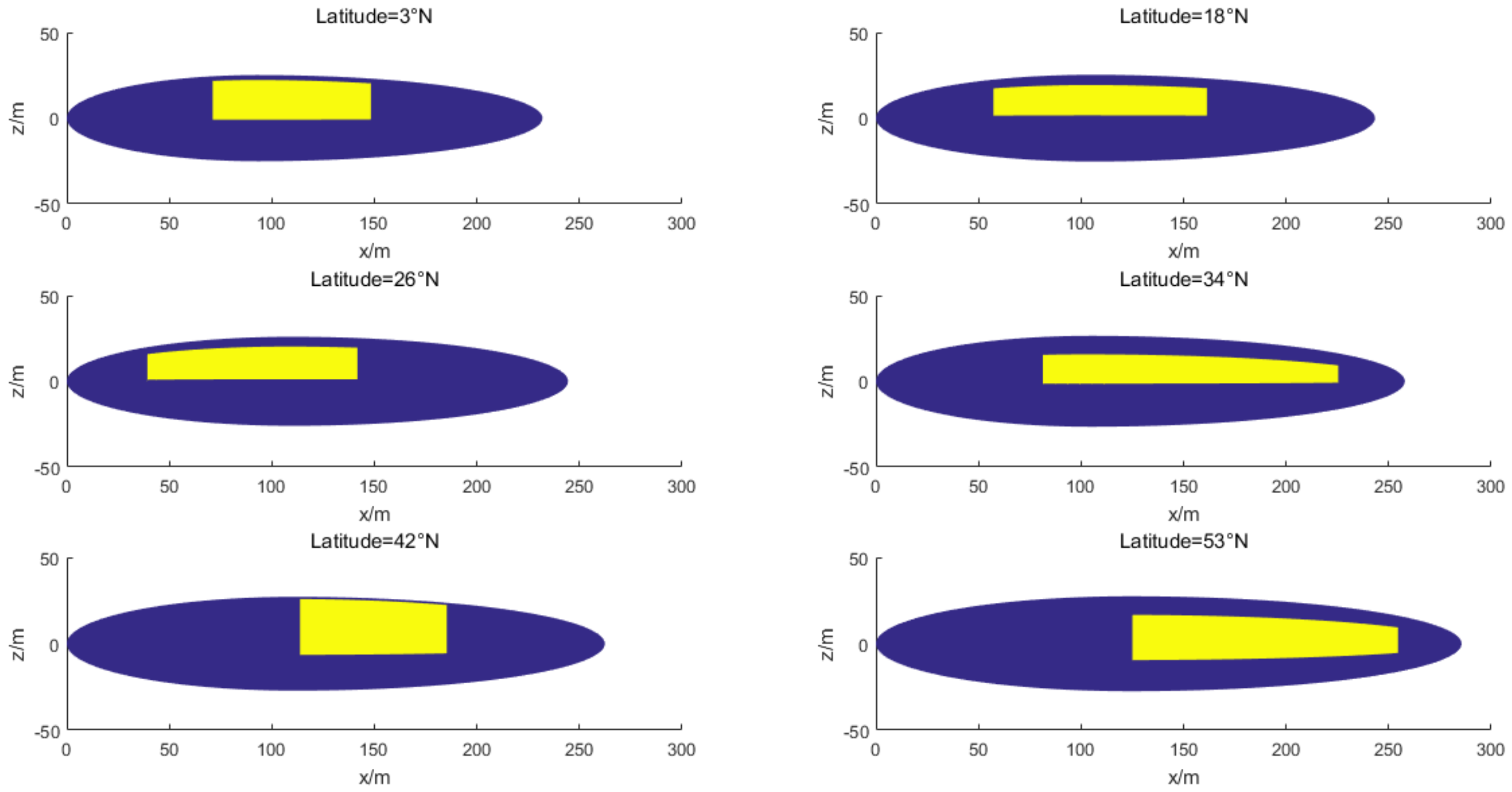
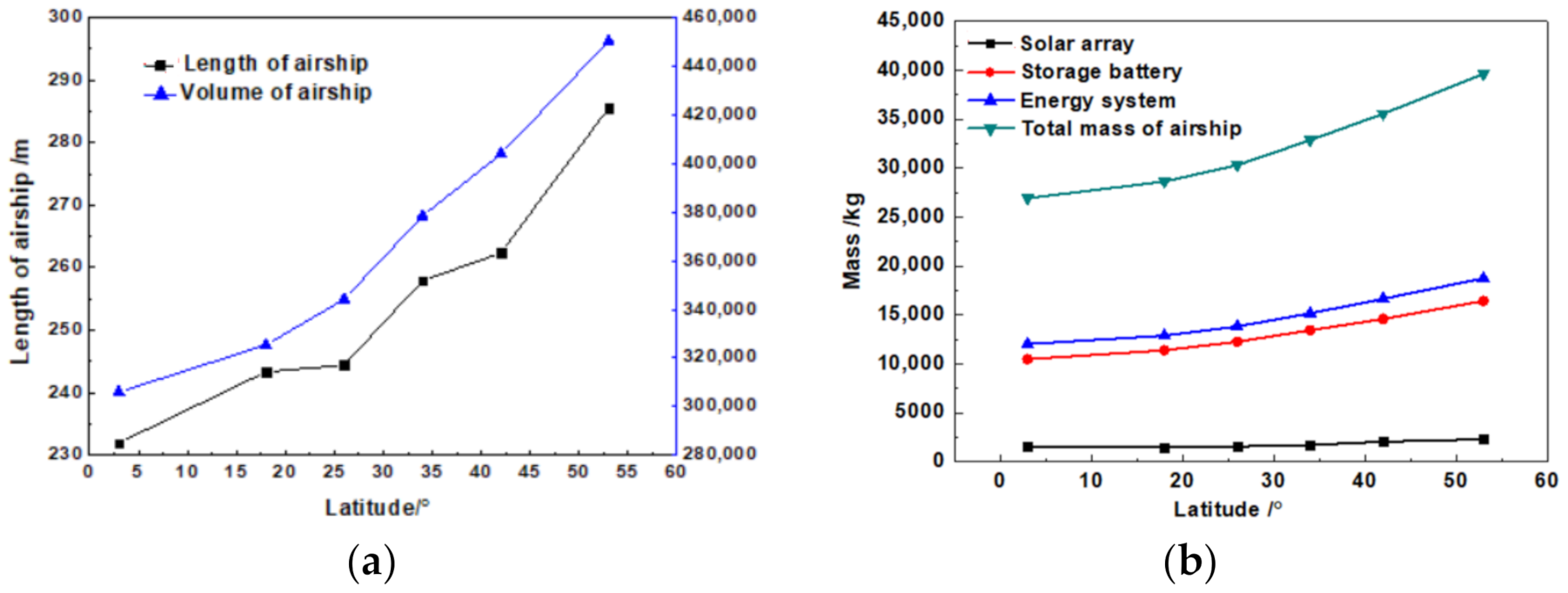
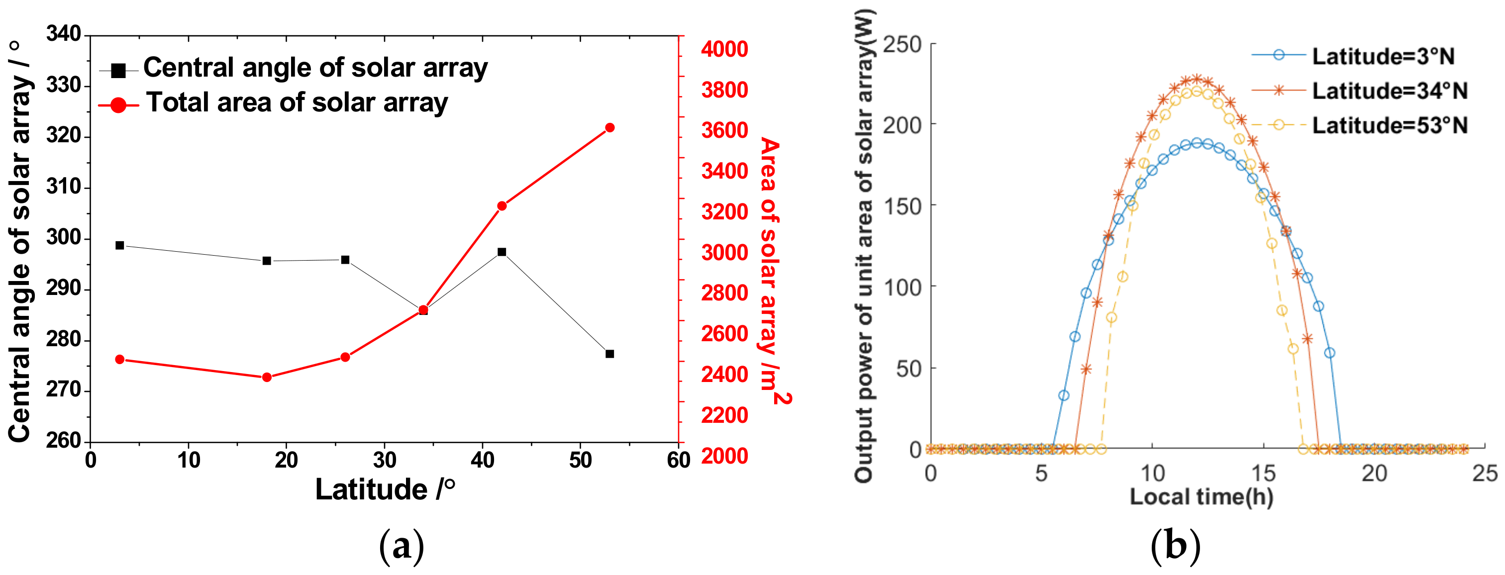
4.2. Effects of Latitudes

Generally, a stratospheric airship is designed to operate at a specific location (latitude, longitude, and altitude) for station-keeping. In this section, the effects of latitude on the optimization results of airship and corresponding solar array layouts are investigated. Design condition (except parameter of the latitude), variables and design space are the same with parameters listed in Section 3.2 and Section 4.1. The latitude ($\varphi$) in each case is 3° N, 18° N, 28° N, 34° N, 42° N and 53° N, respectively.

Figure 12 shows the variations of airship shape and solar array layouts. It can be observed that the optimized shape and size of the airship varies significantly with latitudes. The layout and area of the solar array also differs much with the latitudes. Figure 13 shows the size and mass of the airship for different latitudes. It can be observed from Figure 13a that the volume and length of the airship increase rapidly with the increase in latitudes. This is mainly because solar radiation decreases, and a larger solar array is required with the increase in latitudes. As shown in Figure 13b, the increase in the mass of the storage battery contributes most to the increase in mass of the energy system. This is because with the increase in latitudes, the nighttime becomes longer, thus a larger storage battery is needed. Compared to the increase in total mass, the increase in solar array area is relatively small. However, although the mass ratio of solar array ($m_{so}/m_{to}$) is relatively low (only about 5%), Its performance of output power affects the general key parameters (such as size and shape) of the airship significantly.

Figure 14 shows the optimized central angles of the solar array (${\theta }_0$), area of the solar array ($S_{so}$) and average output power by unit area of the solar array ($\overline{P}=\frac{P_{so}}{S_{so}}$) for different latitudes. As shown in Figure 14a, ${\theta }_0$ ranges from 277.4° to 298.7°, which indicates that more output power can be obtained when the solar array is located on the upper right side of the airship in the present case. In addition, it can be observed that the total area of the solar array generally increases with latitudes. However, as shown in Figure 14b, the average output power by unit area of solar arrays $\overline{P}$ changes with latitudes in a non-monotonous trend. The lowest and highest peak values of $\overline{P}$ are obtained when the latitude is $3^{°}$ N and ${34}^{°}$ N, respectively. This is due to the comprehensive effect of factors such as the local direct radiation, the local length of daytime and the shape of airship envelope, which again validates the need for multidisciplinary optimization design.

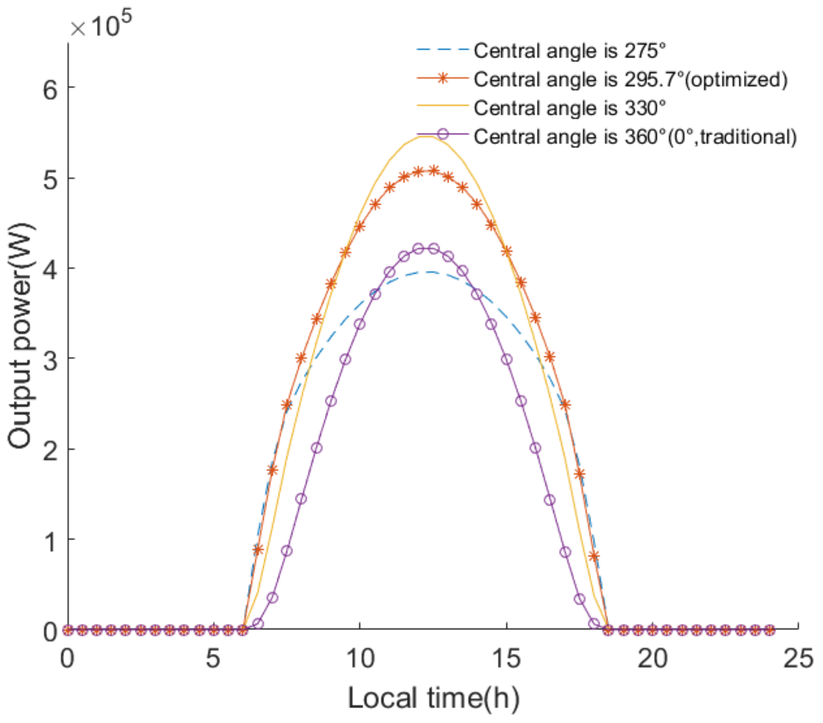
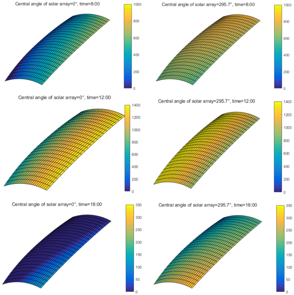
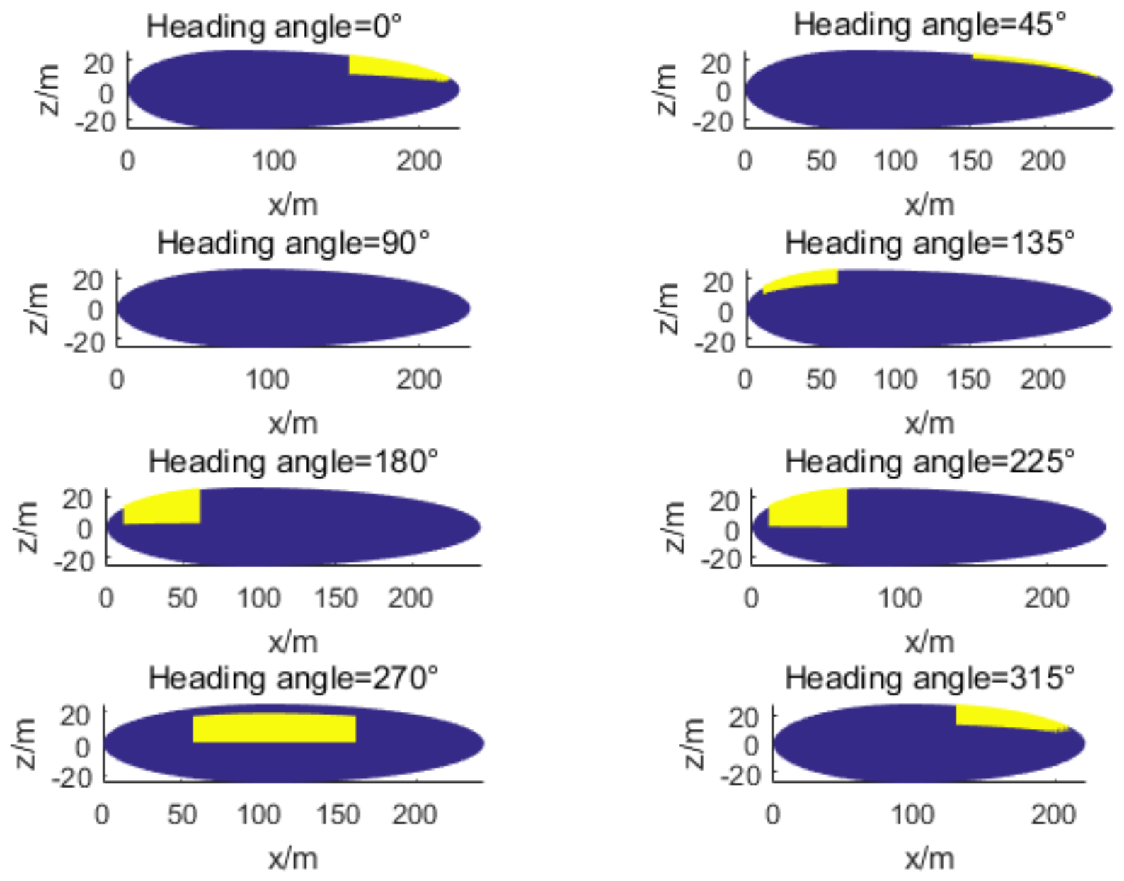
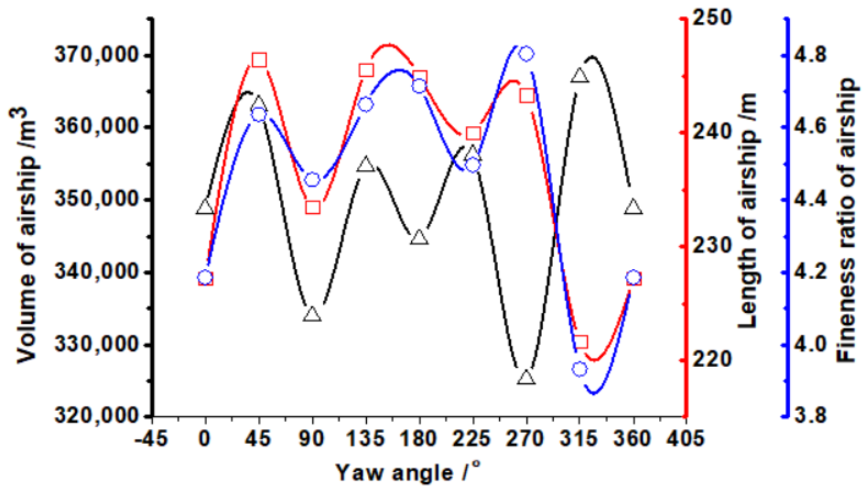
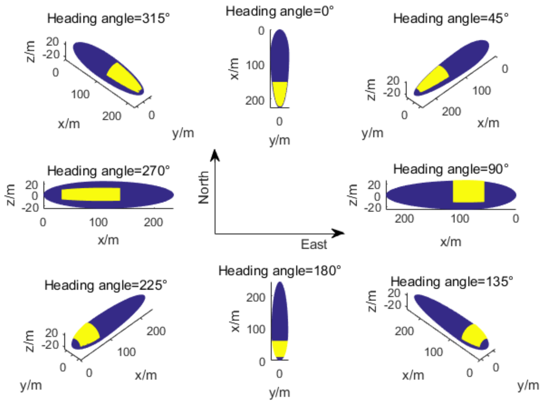
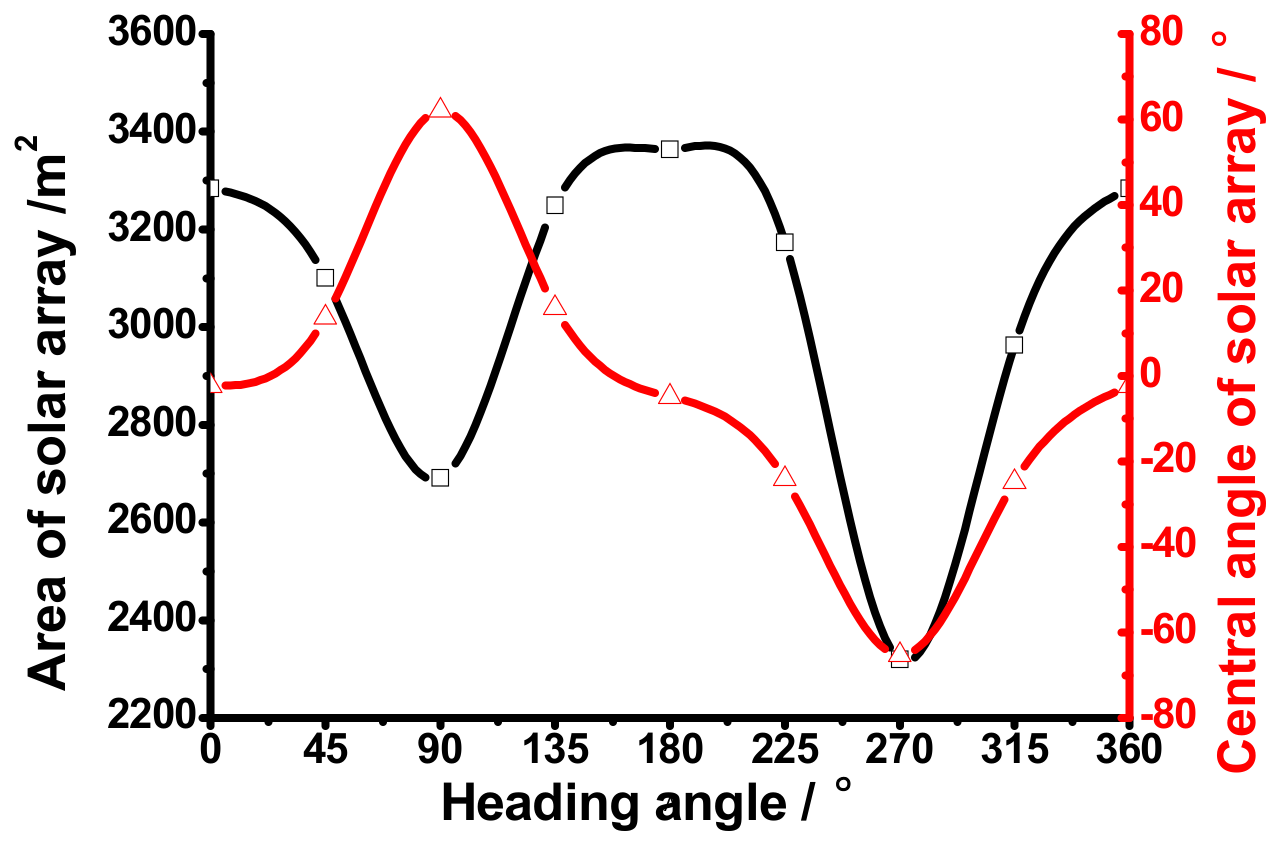
4.3. Effects of Heading Angles

In nearing space, wind directions could be different with seasons or latitudes. Nowadays, due to the current level of subsystems or some engineering challenges (such as reliability of electric devices), an airship is usually designed to meet the specific requirement of station-keeping in certain season. For staying in a certain geographical location and resisting the wind, the wind-resisting strategies such as flight direction (heading angle) in daytime and nighttime are generally determined in advance. However, the heading angle $\psi$ in daytime has effects on the output energy of solar array, which is usually neglected by designers but needs to be considered in the airship design. In this section, the effects of heading angles of airships are investigated.

Figure 15 shows the optimized shape for different heading angles. The latitude is ${18}^{°}$ N. Figure 16 shows the optimized volume, length, and fineness ratio of airships. The optimized shape of airships varies significantly with the heading angles. It is interesting that all curves of volume, length and fineness ratio fluctuate with the heading angles. Taking the optimized volume at $\psi =90°$ (flying from west to east), 270° (flying from east to west) for comparison, the required volume is lower when $\psi =90°$.

Figure 17 shows the optimized layouts of the solar array under different heading angles. Figure 18 shows the optimized area and central angle of solar arrays for different heading angles. It can be observed that all curves are approximately of a sine pattern. The central angles of solar array are nearly anti-symmetric with $\psi =0°$ and 180° (heading north and south, respectively), and nearly symmetric with $\psi =90°$ and 270° (heading east and west, respectively). Taking $0°\le \psi \le 180°$ for example, the central angle initially increases from 2.5° to 71° when $0°\le \psi \le 90°$, and then decreases to −0.18° (${359.82}^{°}$) when heading angle increases to 180°.

Figure 19a shows the optimized mass of airship, solar array, storage battery and whole energy system for different heading angles. Figure 19b shows the corresponding mass ratios of solar array, storage battery and the whole energy system. It can be observed that the optimized mass interestingly fluctuates with the heading angles, which is similar with that of volume. However, although the mass varies significantly with the heading angles, the corresponding mass ratios differ only very little with the variations in heading angles. The mass ratios of solar array, storage battery and whole energy system generally show ranges of 5.3~7.2%, 38.4~41.0% and 45~47%, respectively.

4.4. Effects of Average Resisting Wind Speeds

For higher wind speeds, the airship needs additional energy to provide thrust to overcome the drag. The extra weight of the energy system requires additional buoyancy and larger size to maintain altitude. In this section, the effects of average resisting wind speed ($V_0$) on the optimized configuration of airship are investigated. All the initial parameters are the same as in Section 3.2 and Section 4.1, except the average resisting wind speeds, which are set to be 14, 18, 20, 22 and 25 m/s, respectively. The latitude is ${18}^{°}$ N.

Figure 20 shows the optimized shape and solar array layouts (side view) for different average resisting wind speeds. Figure 21a shows the optimized volume, length and fineness ratios of airships. The optimized volume and length of airships increases rapidly with the increase in resisting wind speeds. It is interesting to note that fineness ratios ($f_r$) almost increase linearly with the increase in resisting wind speeds. This is because in higher wind speeds, drag reduction could be more beneficial than improvements in buoyancy efficiency. Figure 21b shows the optimized area and central angles of solar arrays. The area of solar array $S_{so}$ increases with $V_0$ more rapidly than with volume. This is because the required energy to resist the wind is related to the volume of the airship as much as the speed of the wind. The optimized area of the solar array (2319.7 m²) for $V_0=25$ m/s is about 8.79 times the area of the solar array (264 m²) at $V_0=12$ m/s.

Figure 22 shows the optimized mass and mass ratios of solar array, storage battery, energy system and total mass of airship for different average resisting wind speeds. Although the mass of solar array increases much, mass ratio of solar array only increases by 1.5%, which is from 3.8% to 5.3% in total. However, the mass ratio of the whole energy system increases significantly from 24.9% to 45% (mass increases from 1384 kg to 12,897 kg), which is relatively high. As discussed in Section 2.3, the required capacity ($Q_2$) and mass of energy system are directly related with the output energy of solar array ($Q_3$), which further validates the significance of airship optimization considering the solar array layouts.

5. Conclusions

In the present study, a comprehensive methodology for conceptual design and optimization of a stratospheric airship powered by solar arrays based on the MDO framework is developed. The methodology could achieve the solution with a 19.2% reduction in airship volume with respect to an arbitrary baseline as provided in Table 3. It is also noticed that, although the mass ratio of the solar array is relatively low referring to the total mass of stratospheric airship, its performance of output power significantly affects the optimal configuration of the airship, parameters such as size, shape, and total mass, which indicates that the solar array layout should be seriously optimized in designing a stratospheric airship. It is determined that the circumferential location of the solar array on the airship envelope significantly affects the output performance of solar energy and the size of airship. Therefore, coupling of the central angle of the solar array in design optimization methodology is essential. In addition, under the same payload and other operating conditions, results show that the size of the airship and area of the solar array increase with latitudes, and the optimal solar layout and corresponding central angle also varies. The required area of the solar array and size of the airship fluctuate in an approximate sinusoidal pattern with heading angles, which indicates that the heading angle is an important factor that needs to be considered in the design of stratospheric airship powered by solar arrays.

References

1. Tang, J.; Xie, W.; Wang, X.; Chen, C. Simulation and Analysis of Fluid–Solid–Thermal Unidirectional Coupling of Near-Space Airship. Aerospace 2022, 9, 439. [Google Scholar] [CrossRef]
2. Liu, S.; Sang, Y. Underactuated Stratospheric Airship Trajectory Control Using an Adaptive Integral Backstepping Approach. J. Aircr. 2018, 55, 2357–2371. [Google Scholar] [CrossRef]
3. Alam, M.I.; Pant, R.S. Estimation of Volumetric Drag Coefficient of Two-Dimensional Body of Revolution. J. Aircr. 2019, 56, 2080–2082. [Google Scholar] [CrossRef]
4. Tang, J.; Wang, X.; Duan, D.; Xie, W. Optimisation and analysis of efficiency for contra-rotating propellers for high-altitude airships. Aeronaut. J. 2019, 123, 706–726. [Google Scholar] [CrossRef]
5. Yoder, C.D.; Agrawal, S.; Motes, A.G.; Mazzoleni, A.P. Aerodynamic Tethered Sails for Scientific Balloon Trajectory Control: Small-Scale Experimental Demonstration. J. Aircr. 2021, 58, 1. [Google Scholar] [CrossRef]
6. Robyr, J.-L.; Bourquin, V.; Goetschi, D.; Schroeter, N.; Baltensperger, R. Modeling the Vertical Motion of a Zero Pressure Gas Balloon. J. Aircr. 2020, 57, 991–994. [Google Scholar] [CrossRef]
7. Colozza, A. PV/regenerative fuel cell high altitude airship feasibility study. In Proceedings of the 2nd AIAA “Unmanned Unlimited” Conference and Workshop & Exhibit, AIAA 2003-6663, San Diego, CA, USA, 15–18 September 2003. [Google Scholar] [CrossRef]
8. Hoshino, T.; Okaya, S.; Fujiwara, T.; Miwa, S.; Nomura, Y.; Naito, H.; Eguchi, K. Design and analysis of solar power system for SPF airship operations. In Proceedings of the 13th AIAA Lighter-Than Air Technology Conference, Norfolk, VA, USA, 28 June–1 July 1999. [Google Scholar] [CrossRef]
9. Wang, H.; Song, B.; Zuo, L. Effect of High-Altitude Airship’s Attitude on Performance of its Energy System. J. Aircr. 2007, 44, 2077–2080. [Google Scholar] [CrossRef]
10. Zhang, Y.; Li, J.; Lv, M.; Tan, D.; Zhu, W.; Sun, K. Simplified Analytical Model for Investigating the Output Power of Solar Array on Stratospheric Airship. Int. J. Aeronaut. Space Sci. 2016, 17, 432–441. [Google Scholar] [CrossRef]
11. Du, H.; Zhu, W.; Wu, Y.; Zhang, L.; Li, J.; Lv, M. Effect of angular losses on the output performance of solar array on long-endurance stratospheric airship. Energy Convers. Manag. 2017, 147, 135–144. [Google Scholar] [CrossRef]
12. Zhu, W.; Li, J.; Xu, Y. Optimum attitude planning of near-space solar powered airship. Aerosp. Sci. Technol. 2019, 84, 291–305. [Google Scholar] [CrossRef]
13. Alam, M.I.; Pant, R.S. A multi-node model for transient heat transfer analysis of stratospheric airships. Adv. Space Res. 2017, 59, 3023–3035. [Google Scholar] [CrossRef]
14. Alam, M.I.; Pant, R.S. Multidisciplinary approach for solar area optimization of high altitude airships. Energy Convers. Manag. 2018, 164, 301–310. [Google Scholar] [CrossRef]
15. Garg, A.; Burnwal, S.; Pallapothu, A.; Alawa, R.; Ghosh, A. Solar Panel Area Estimation and Optimization for Geostationary Stratospheric Airships. In Proceedings of the 11th AIAA Aviation Technology, Integration, and Operations (ATIO) Conference, Virginia Beach, VA, USA, 20–22 September 2011. [Google Scholar] [CrossRef]
16. Li, J.; Lv, M.; Sun, K. Optimum area of solar array for stratospheric solar-powered airship. Proc. Inst. Mech. Eng. Part G J. Aerosp. Eng. 2016, 231, 2654–2665. [Google Scholar] [CrossRef]
17. Liang, H.; Zhu, M.; Guo, X.; Zheng, Z. Conceptual Design Optimization of High Altitude Airship in Concurrent Subspace Optimization. In Proceedings of the 50th AIAA Aerospace Sciences Meeting Including the New Horizons Forum and Aerospace Exposition; AIAA 2012-1180, Nashville, TN, USA, 9–12 January 2012. [Google Scholar] [CrossRef]
18. Zhu, W.; Xu, Y.; Li, J.; Du, H.; Zhang, L. Research on optimal solar array layout for near-space airship with thermal effect. Sol. Energy 2018, 170, 1–13. [Google Scholar] [CrossRef]
19. Wang, Q.-B.; Chen, J.-A.; Fu, G.-Y.; Duan, D.-P. An approach for shape optimization of stratosphere airships based on multidisciplinary design optimization. J. Zhejiang Univ. A 2009, 10, 1609–1616. [Google Scholar] [CrossRef]
20. Trancossi, M.; Dumas, A.; Madonia, M. Energy and Mission Optimization of an Airship by Constructal Design for Efficiency Method. In Proceedings of the ASME 2013 International Mechanical Engineering Congress and Exposition, San Diego, CA, USA, 15–21 November 2013. [Google Scholar] [CrossRef]
21. Shan, C.; Lv, M.; Sun, K.; Gao, J. Analysis of energy system configuration and energy balance for stratospheric airship based on position energy storage strategy. Aerosp. Sci. Technol. 2020, 101, 105844. [Google Scholar] [CrossRef]
22. Ceruti, A.; Gambacorta, D.; Marzocca, P. Unconventional hybrid airships design optimization accounting for added masses. Aerosp. Sci. Technol. 2018, 72, 164–173. [Google Scholar] [CrossRef]
23. Meng, J.; Li, M.; Ma, N.; Liu, L. Multidisciplinary design optimization of a lift-type hybrid airship. J. Beijing Univ. Aeronaut. Astronaut. 2021, 47, 72–83. [Google Scholar] [CrossRef]
24. Zhang, L.; Lv, M.; Zhu, W.; Du, H.; Meng, J.; Li, J. Mission-based multidisciplinary optimization of solar-powered hybrid airship. Energy Convers. Manag. 2019, 185, 44–54. [Google Scholar] [CrossRef]
25. Tang, J.; Duan, D.; Xie, W. Shape Exploration and Multidisciplinary Optimization Method of Semirigid Nearing Space Airships. J. Aircr. 2021, 59, 946–963. [Google Scholar] [CrossRef]
26. Zhang, L.; Lv, M.; Meng, J.; Du, H. Conceptual design and analysis of hybrid airships with renewable energy. Proc. Inst. Mech. Eng. Part G J. Aerosp. Eng. 2018, 232, 2144–2159. [Google Scholar] [CrossRef]
27. Zhang, L.; Lv, M.; Meng, J.; Du, H. Optimization of solar-powered hybrid airship conceptual design. Aerosp. Sci. Technol. 2017, 65, 54–61. [Google Scholar] [CrossRef]
28. Lv, M.; Li, J.; Du, H.; Zhu, W.; Meng, J. Solar array layout optimization for stratospheric airships using numerical method. Energy Convers. Manag. 2017, 135, 160–169. [Google Scholar] [CrossRef]
29. Lv, M.; Li, J.; Zhu, W.; Du, H.; Meng, J.; Sun, K. A theoretical study of rotatable renewable energy system for stratospheric airship. Energy Convers. Manag. 2017, 140, 51–61. [Google Scholar] [CrossRef]
30. Zhang, L.; Zhu, W.; Du, H.; Lv, M. Multidisciplinary design of high altitude airship based on solar energy optimization. Aerosp. Sci. Technol. 2021, 110, 106440. [Google Scholar] [CrossRef]
31. Pant, R. A Methodology for Determination of Baseline Specifications of a Non-Rigid Airship. In Proceedings of the AIAA’s 3rd Annual Aviation Technology, Integration, and Operations Conference (ATIO), AIAA 2003-6830, Denver, CO, USA, 17–19 November 2003. [Google Scholar] [CrossRef]
32. Yang, X.; Liu, D. Renewable power system simulation and endurance analysis for stratospheric airships. Renew. Energy 2017, 113, 1070–1076. [Google Scholar] [CrossRef]
33. Farley, R. Balloon Ascent: 3-D Simulation Tool for the Ascent and Float of High-Altitude Balloons. In Proceedings of the AIAA’s 5th Aviation, Technology, Integration, and Operations Conference (ATIO), AIAA 2005-7412, Arlington, VA, USA, 26–28 September 2005. [Google Scholar] [CrossRef]
34. Kalogirou, S. Solar Energy Engineering—Processes and Systems, 1st ed.; Elsevier: London, UK, 2009. [Google Scholar]
35. Palumbo, R.; Russo, M.; Filippone, E.; Corraro, F. ACHAB: Analysis Code for High-Altitude Balloons. In Proceedings of the AIAA Atmospheric Flight Mechanics Conference and Exhibit, AIAA 2007-6642, Hilton Head, SC, USA, 20–23 August 2007. [Google Scholar] [CrossRef]
36. Gui, W.; Li, T.; Lu, Y. Improvement of solar position formula and its application. Water Resour. Power 2011, 29, 213–216. [Google Scholar]
37. Hoerner, S. Fluid-Dynamic Drag: Practical Information on Aerodynamic Drag and Hydrodynamic Resistance; Fluid Dynamics: Midland Park, NJ, USA, 1965; Available online: https://n2t.net/ark:/13960/t57f0bk2j (accessed on 1 January 2022).
38. Cheeseman, I. Airship Technology; Cambridge University Press: Cambridge, UK, 2012. [Google Scholar]
39. Yang, B. Formulization of standard atmospheric parameters. J. Astronaut. 1983, 1, 83–86. [Google Scholar]
40. Colozza, A.; Dolce, J. Initial Feasibility Assessment of a High Altitude Long Endurance Airship, NASA/CR. 2003. Available online: https://ntrs.nasa.gov/citations/20040021326 (accessed on 11 December 2022).
41. Zhang, W.-W.; Qi, H.; Yu, Z.-Q.; He, M.-J.; Ren, Y.-T.; Li, Y. Optimization configuration of selective solar absorber using multi-island genetic algorithm. Sol. Energy 2021, 224, 947–955. [Google Scholar] [CrossRef]
42. Schittkowski, K. NLPQL: A fortran subroutine solving constrained nonlinear programming problems. Ann. Oper. Res. 1986, 5, 485–500. [Google Scholar] [CrossRef]
Figure 1. Research plan.
Aerospace 10 00043 g001
Figure 2. Simplified geometric parameters of an airship.
Aerospace 10 00043 g002
Figure 3. Sketch of the position of the sun.
Aerospace 10 00043 g003
Figure 4. Sketch of the body–axis coordinate system and the solar array cell.
Aerospace 10 00043 g004
Figure 5. Sketch of energy balance.
Aerospace 10 00043 g005
Figure 6. Flowchart of optimization.
Aerospace 10 00043 g006
Figure 7. Comparison of convergence history for hybrid algorithm, MIGA and NLPQL.
Aerospace 10 00043 g007
Figure 8. Comparison of the shape and platform of the solar array for baseline and the optimized airship.
Aerospace 10 00043 g008
Figure 9. Comparison of instantaneous output power and requested power for baseline and optimized airship.
Aerospace 10 00043 g009
Figure 10. Comparison of instantaneous output power of solar array for different central angle.
Aerospace 10 00043 g010
Figure 11. Comparison of instantaneous direct solar radiation distribution on the solar array for central angle θ 0 = 0 ° (traditional configuration) and θ 0 = 295.7 ° (optimized solution).
Aerospace 10 00043 g011
Figure 12. Envelope and solar array geometry for winter solstice in different latitude.
Aerospace 10 00043 g012
Figure 13. (a) Optimized volume and length of airship for different latitudes. (b) The mass of solar array, storage battery, energy system and total mass of the airship for different latitudes.
Aerospace 10 00043 g013
Figure 14. (a) The optimized area and central angle of solar arrays for different latitudes. (b) Unit area of solar arrays for different latitudes.
Aerospace 10 00043 g014
Figure 15. The optimized shape of airship (side view) for different heading angles.
Aerospace 10 00043 g015
Figure 16. The optimized volume, length, and fineness ratio of airships for different heading angles.
Aerospace 10 00043 g016
Figure 17. The optimized layouts of the solar array for different heading angles.
Aerospace 10 00043 g017
Figure 18. The optimized area and central angles of solar arrays for different heading angles.
Aerospace 10 00043 g018
Figure 19. (a) The optimized total mass of airship, mass of solar array, mass of storage and mass of energy system for different heading angles. (b) The optimized mass ratios of solar array, storage battery and whole energy system for different heading angles.
Aerospace 10 00043 g019
Figure 20. The optimized shape of the airship and layout of the solar array (side view) for different average resisting wind speeds.
Aerospace 10 00043 g020
Figure 21. (a) The optimized volume, length, and fineness ratio of airships. (b) The optimized area and central angles of solar arrays for different average resisting wind speeds.
Aerospace 10 00043 g021
Figure 22. (a) The optimized mass of solar array, storage battery, energy system and total mass of airship. (b) Optimized mass ratios of solar array, storage battery and energy system for different average resisting wind speeds.
Aerospace 10 00043 g022