
Mission Design and Orbit-Attitude Control Algorithms Development of Multistatic SAR Satellites for Very-High-Resolution Stripmap Imaging

Abstract
:1. Introduction
2. Preliminary Design of a Multistatic SAR Formation System for VHRSI
2.1. Top-Level Requirements of Multistatic SAR System
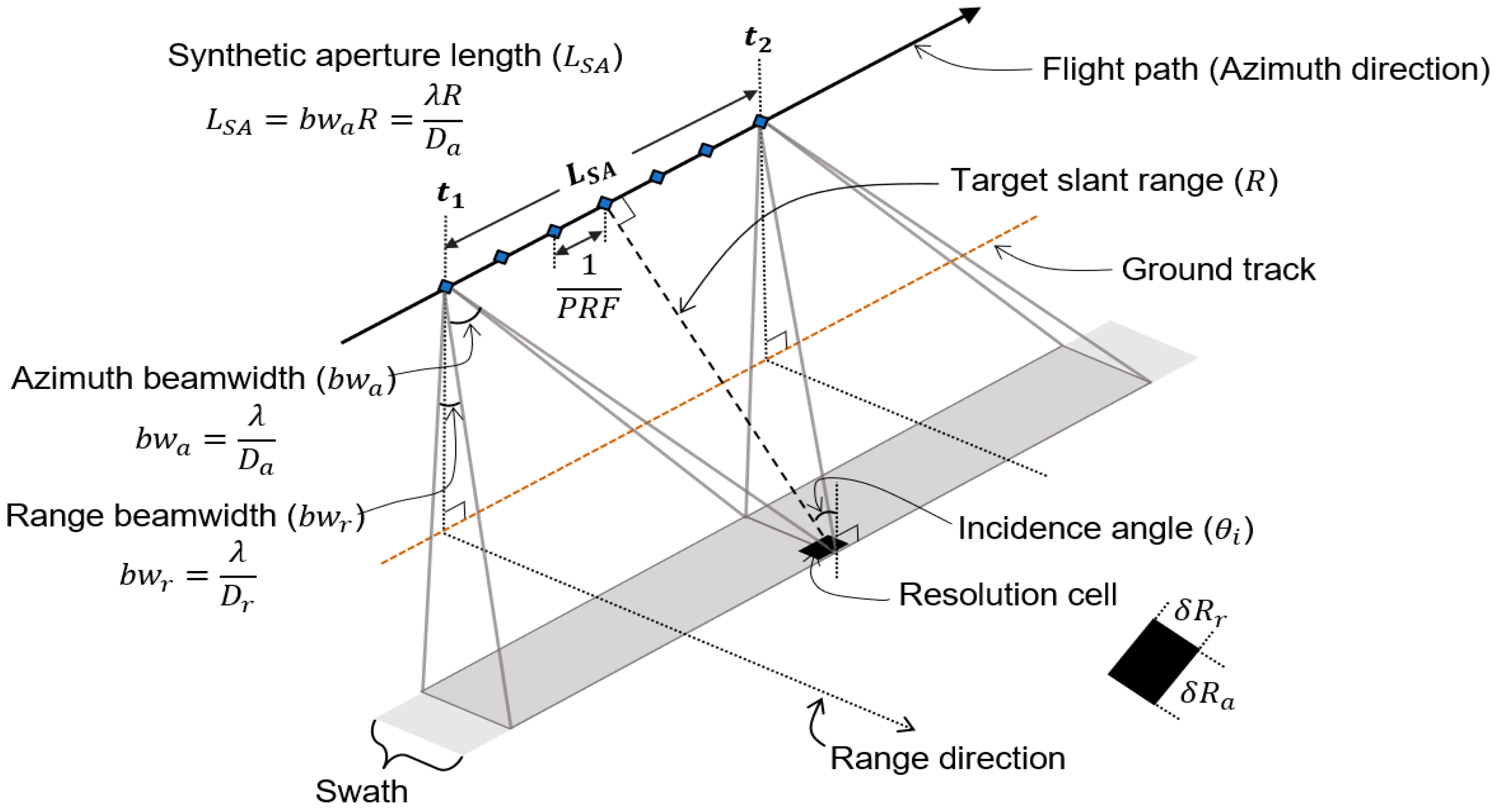
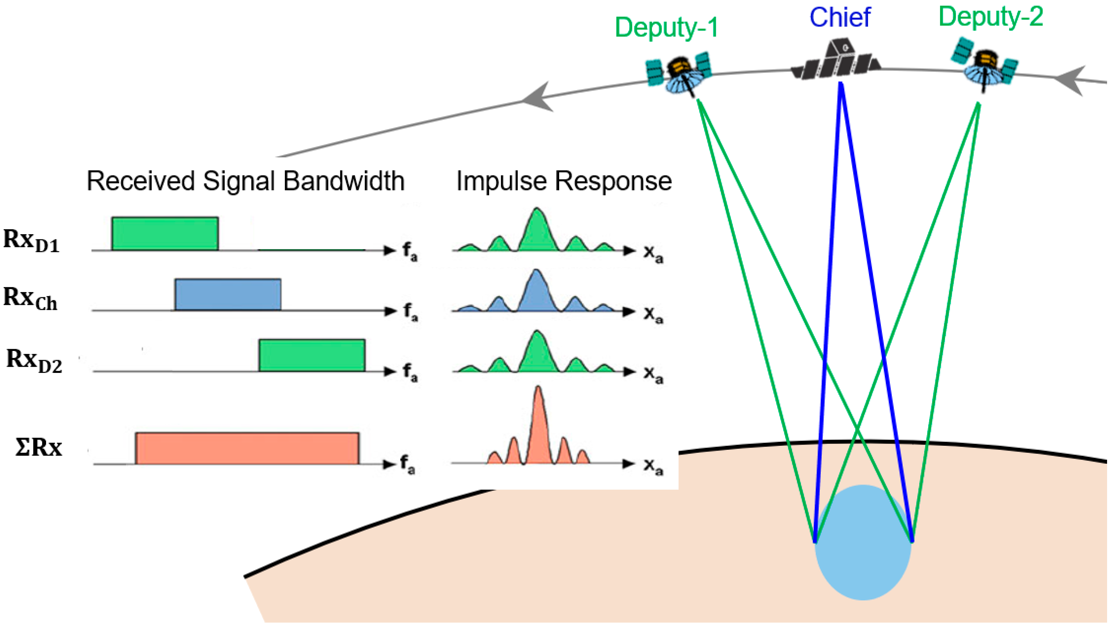
2.2. Methodology for Improving the Resolution of a SAR Image
2.3. Formation Design of Multistatic SAR Satellites
3. Design of the Relative-Orbit-Control Algorithm for Multistatic SAR Formation-Flying
- (1)
- The relative distance (baseline) should be maintained at 6000 ± 100 m for the along-track direction. Here, the error criterion of 100 m is set as half of the ground-station based relative orbital control error of the multistatic SAR mission of TerraSAR-X and TanDEM-X [31].
- (2)
- The magnitude of the thrust used for relative orbit control shall not exceed the performance of the thruster suitable for microsatellites.
- (3)
- The total used during the lifetime of the satellite shall not exceed the total fuel of the thrusters.
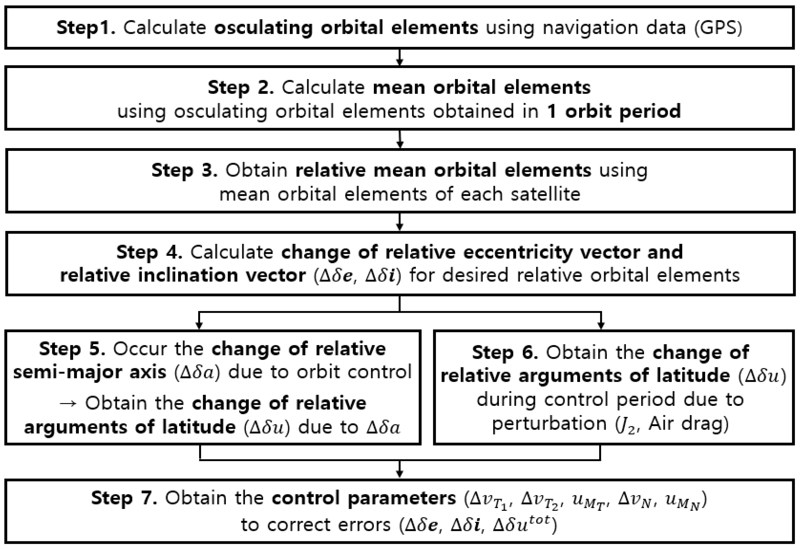
3.1. Relative Orbit Control Algorithm for the Along-Track Formation Maintenance
3.1.1. Calculations of the Mean Relative Orbital Elements (Steps 1, 2, and 3 in Figure 4)
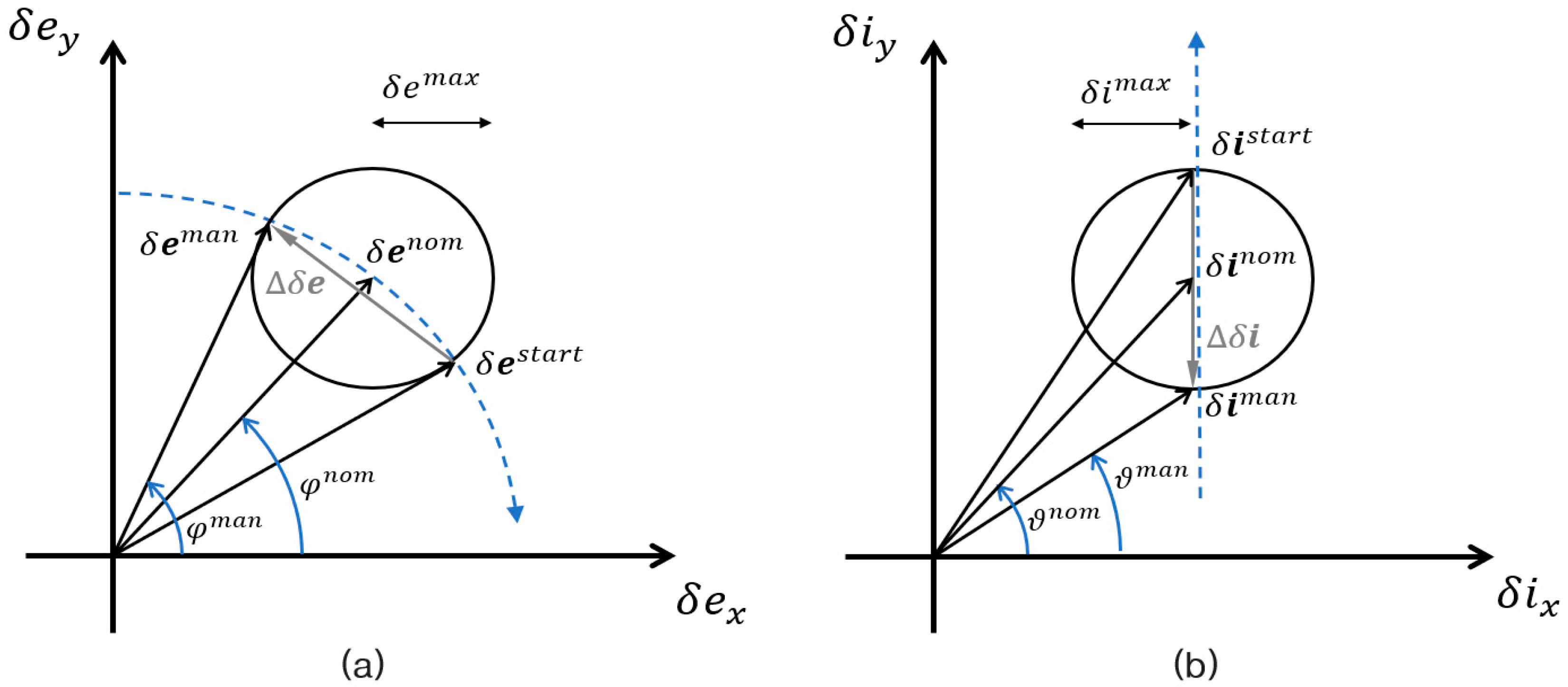
3.1.2. Calculation of the Control Value of Relative Eccentricity and Inclination ( and ) for Desired Relative Orbit Motion (Step 4 in Figure 4)
3.1.3. Calculations of the Control Value of the Relative Semimajor Axis () to Maintain the Desired Relative Mean Argument of Latitude (Steps 5 and 6 in Figure 4)
3.1.4. Calculations of Control Parameters (Step 6 in Figure 4)
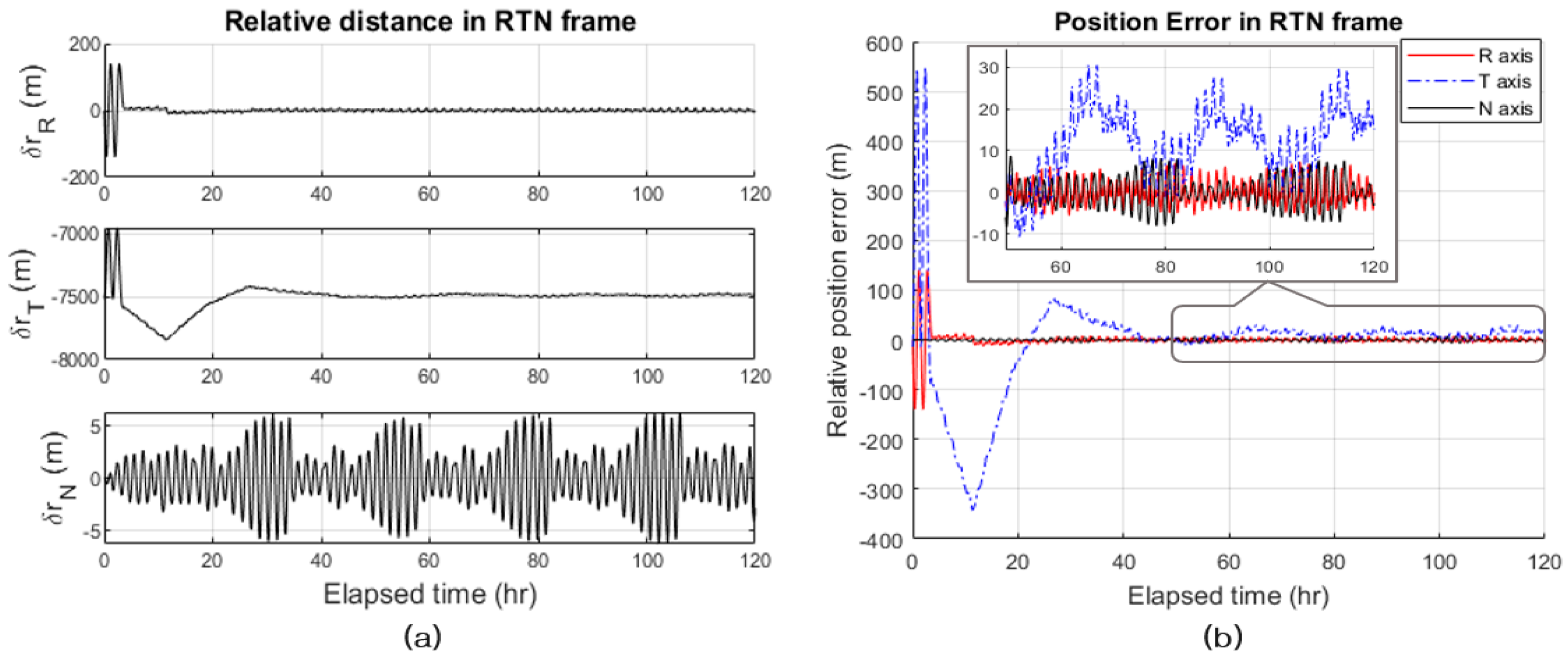
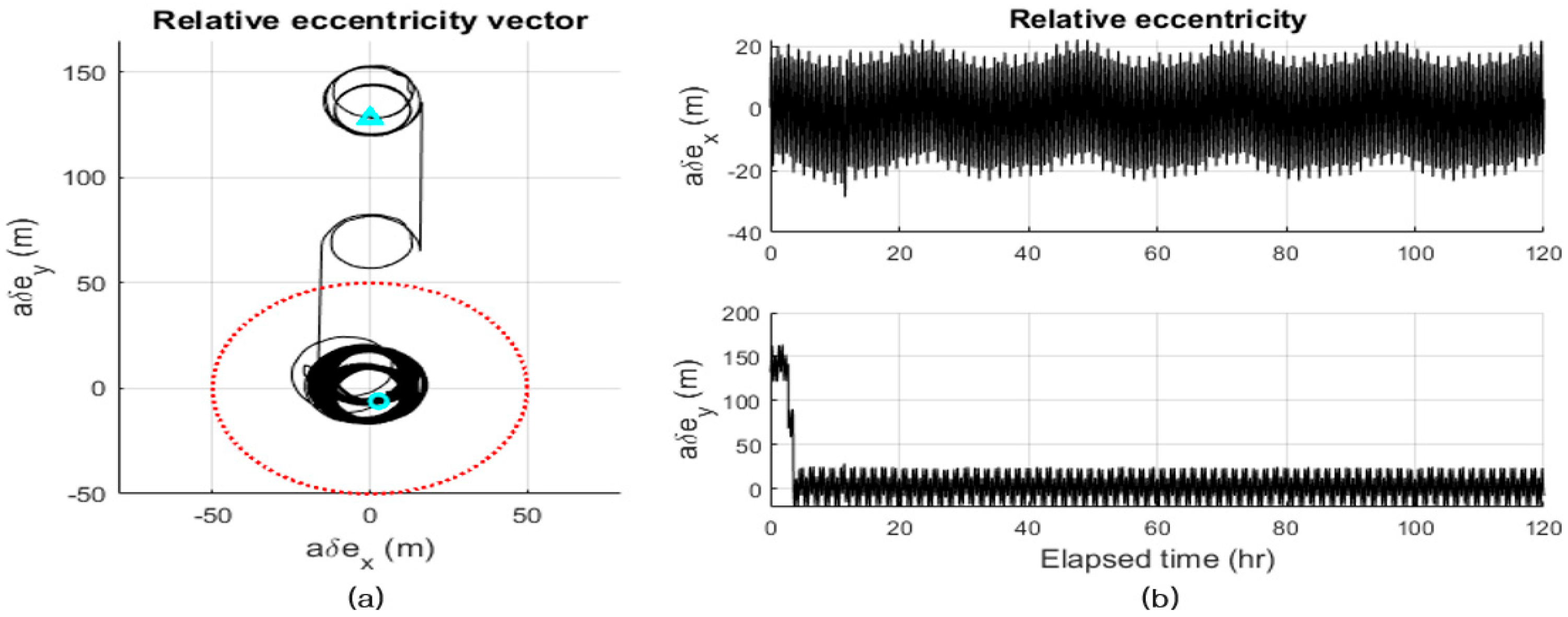
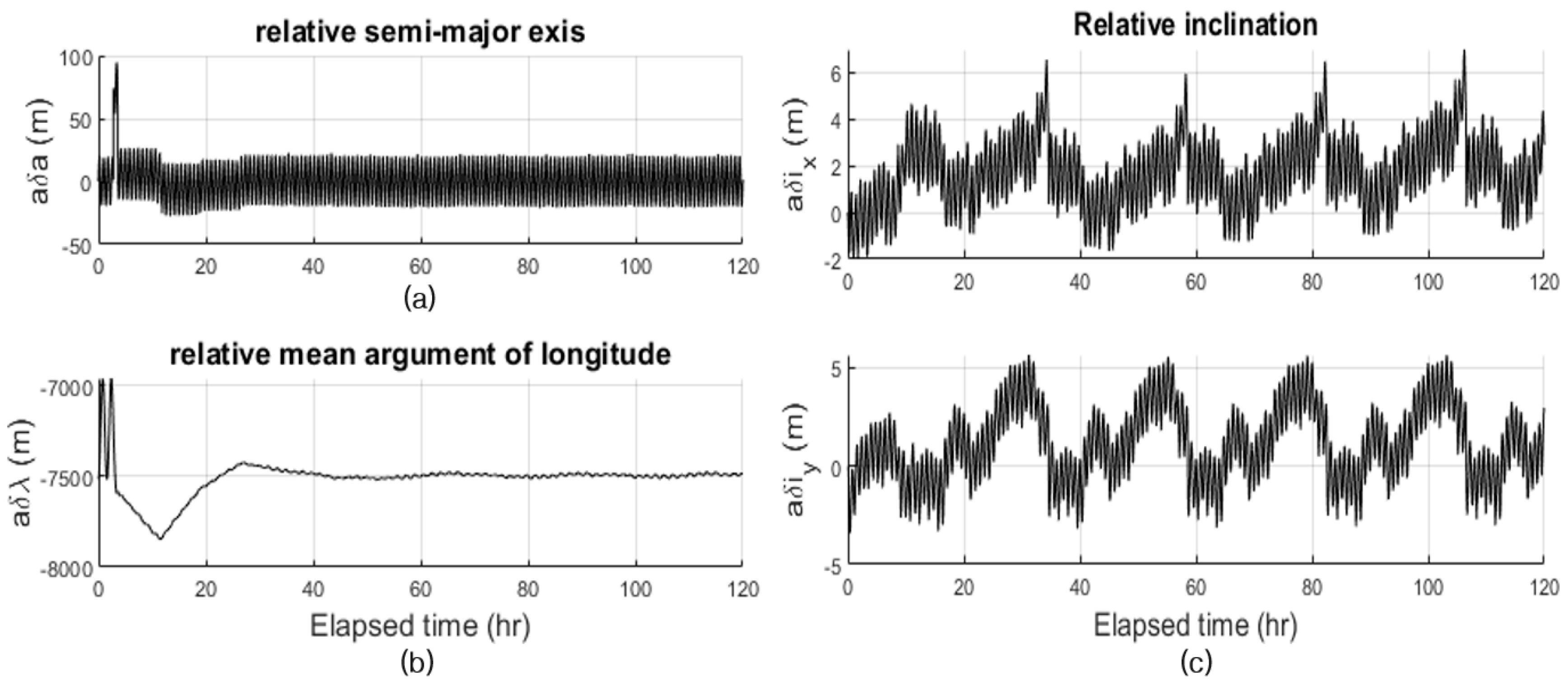
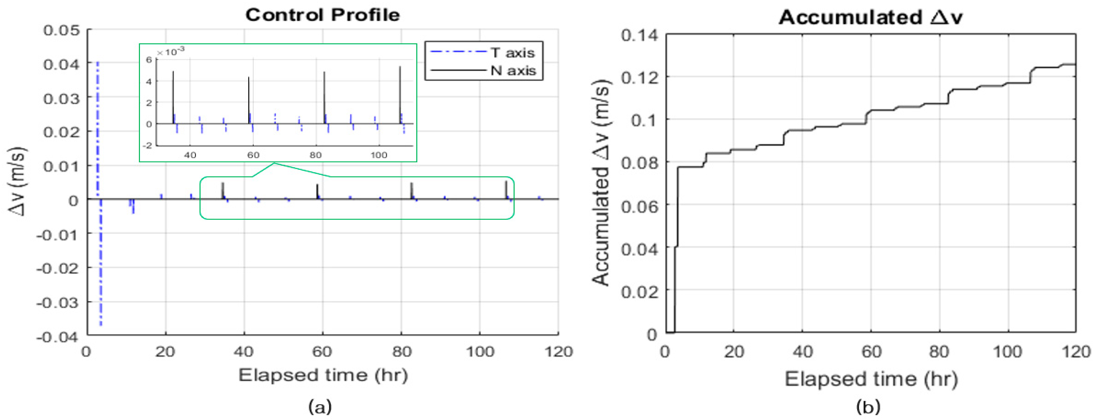
3.2. Numerical Simulations of Relative Orbit Control for the Along-Track Formation Maintenance
3.3. Performance Analysis of Thrusters for Orbit Control
4. Autonomous Attitude Control of Multistatic SAR Satellites for VHRSI
- (1)
- The antenna pointing error through attitude control must be within 0.01° (3σ).
- (2)
- The attitude stability during multistatic SAR imaging must be within 0.0007°/s (3σ).
- (3)
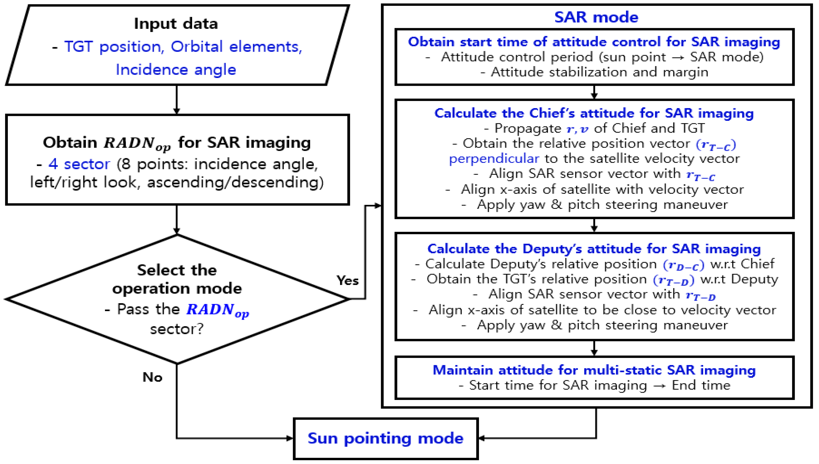
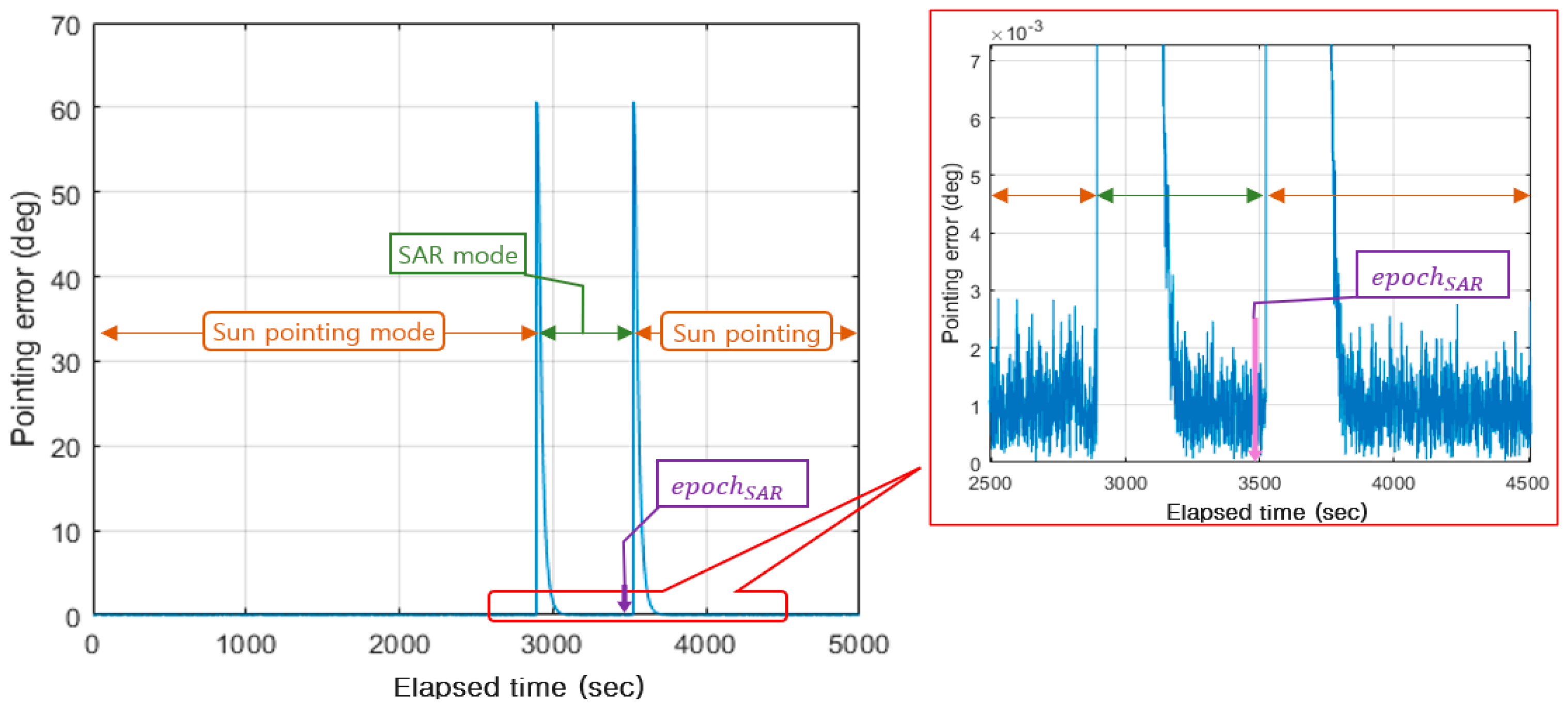
- The attitude control for the multistatic SAR imaging must be completed at least 0.7 s before . Because strip-map SAR imaging synthesizes received signals from the leading edge of the azimuth direction of the transmitted radar beam, SAR imaging starts before half the beam width from the target. Here, denotes a time point when the Doppler shift frequency of the chief satellite with respect to the ground target becomes zero.
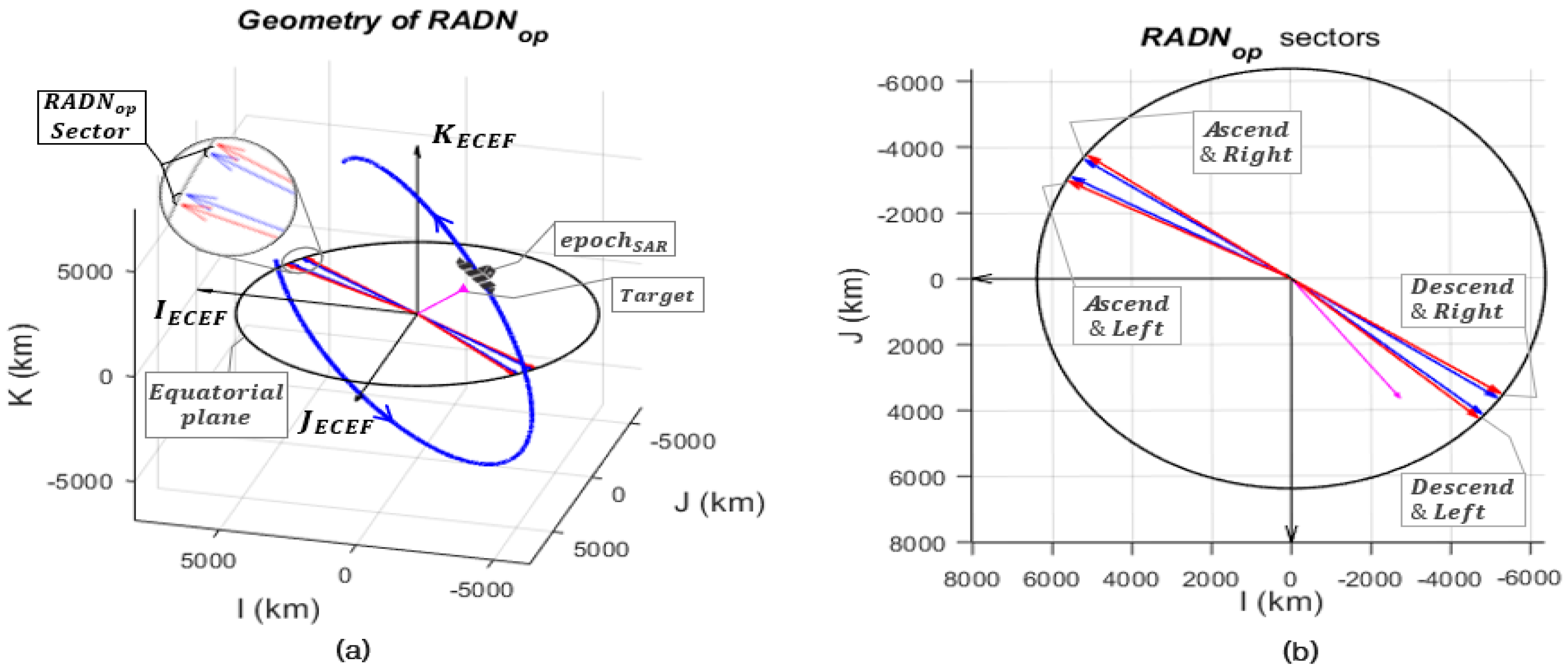
4.1. Concept of the Optimal RADN () Sectors
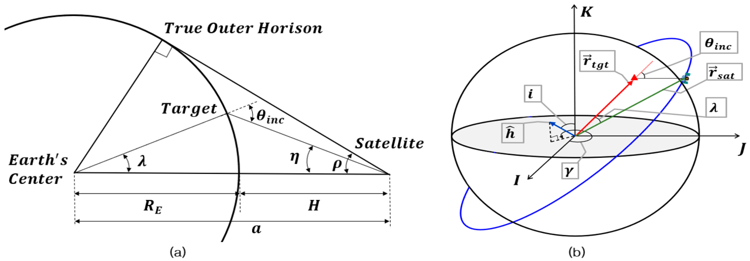
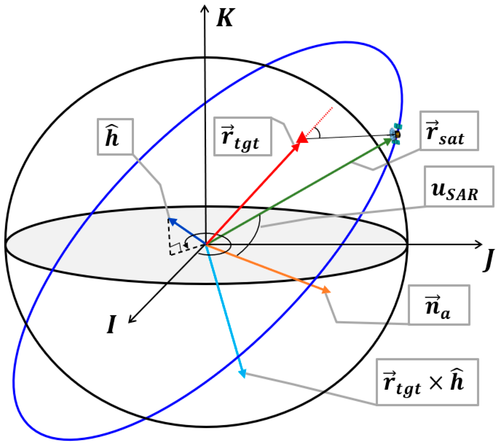
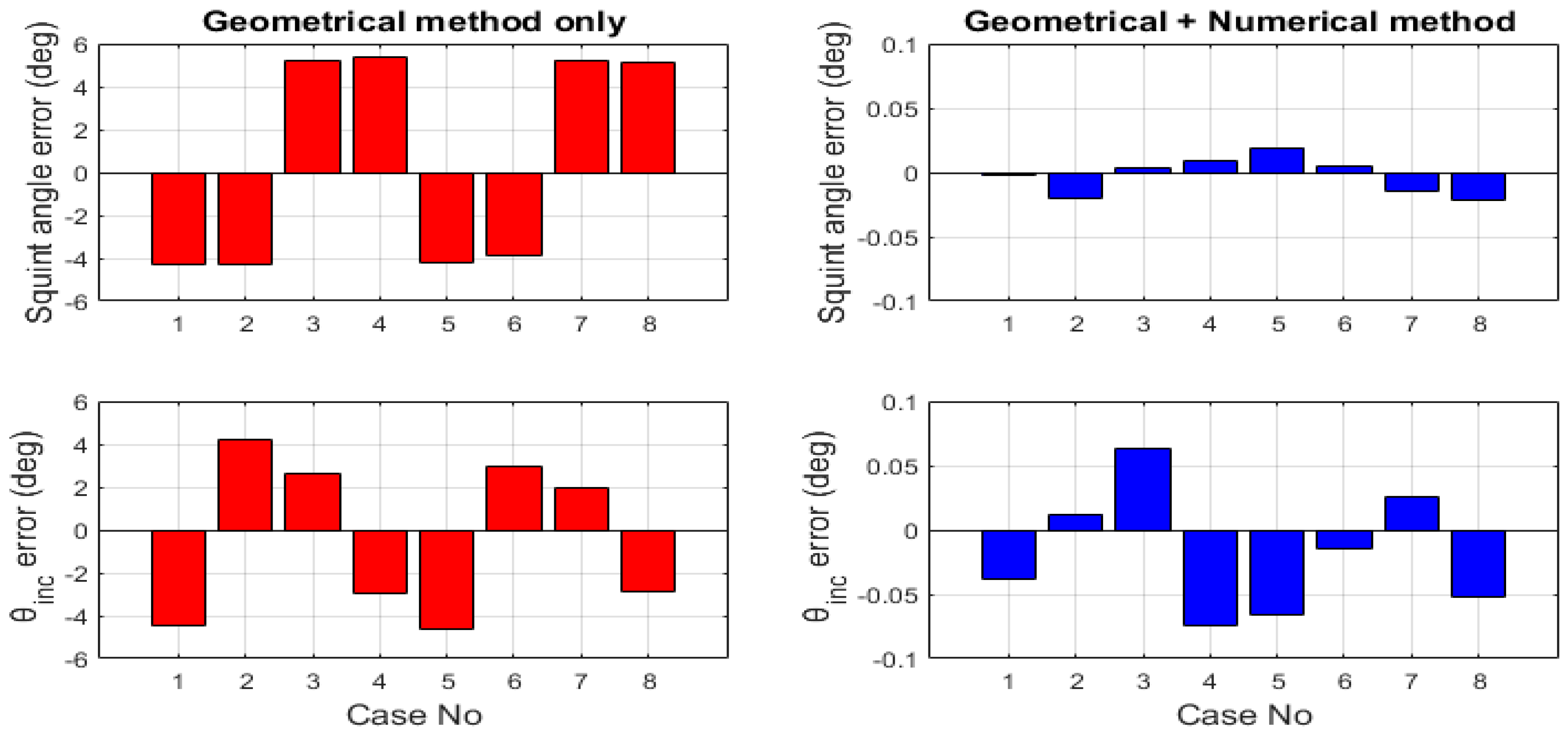
4.1.1. Calculation of Using the Geometric Method
4.1.2. Obtaining the Precise Using a Numerical Method
4.2. Attitude Control Strategy for Multistatic SAR Imaging
4.3. Design of the Attitude-Control Algorithm
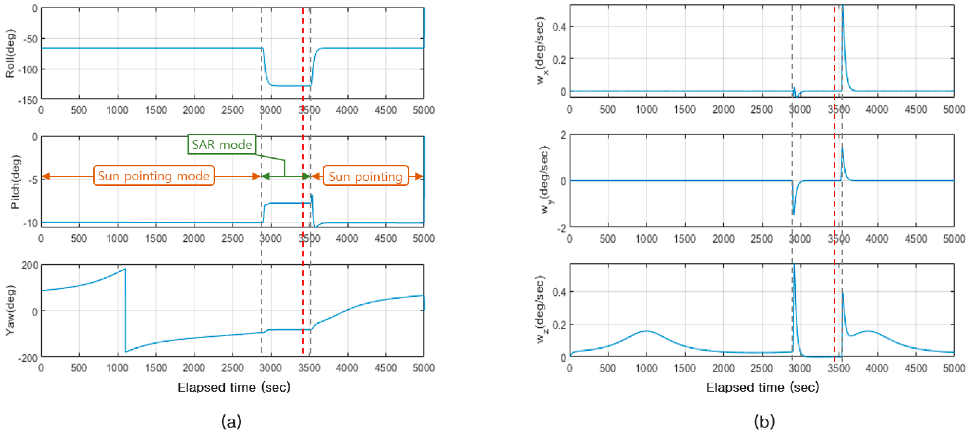
4.4. Numerical Simulations of Autonomous Attitude Control
5. Performance Verification and Image Analysis of a Multistatic SAR System for VHRSI
5.1. Performance Analysis of the Preliminary Design of a Multistatic SAR System
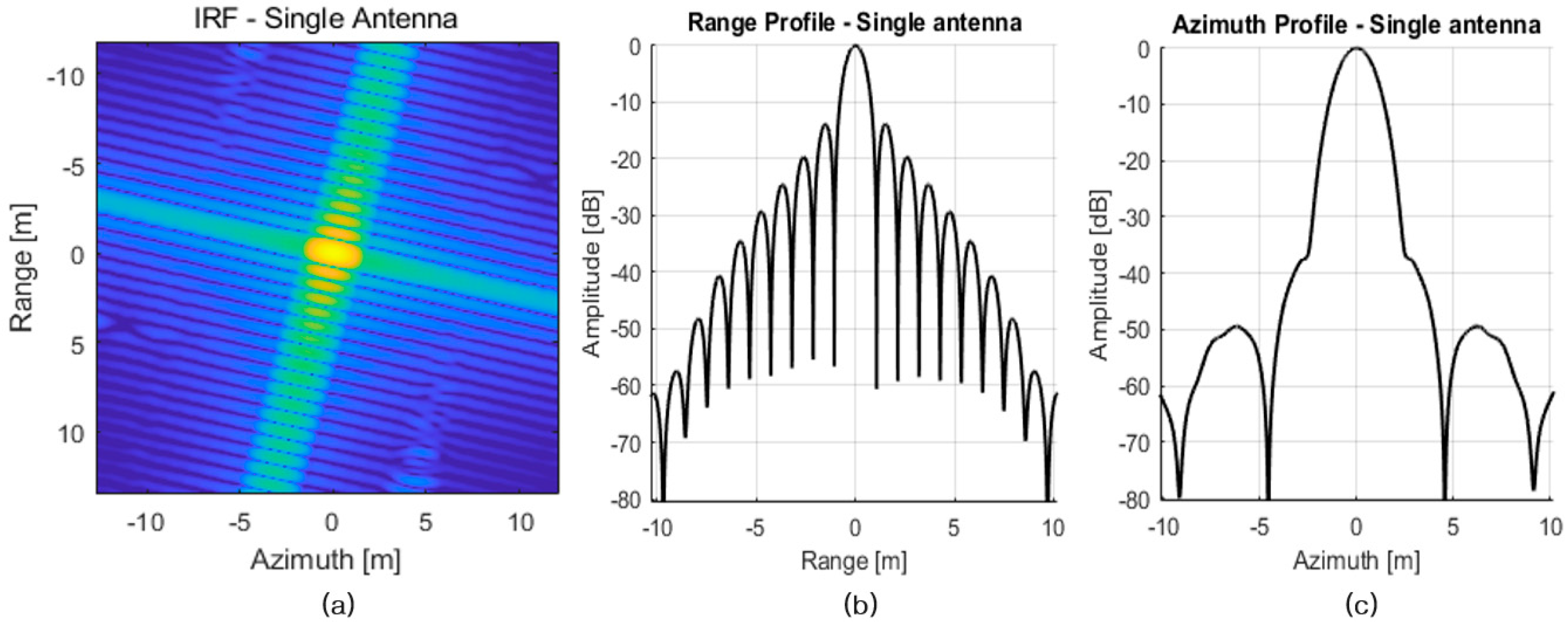
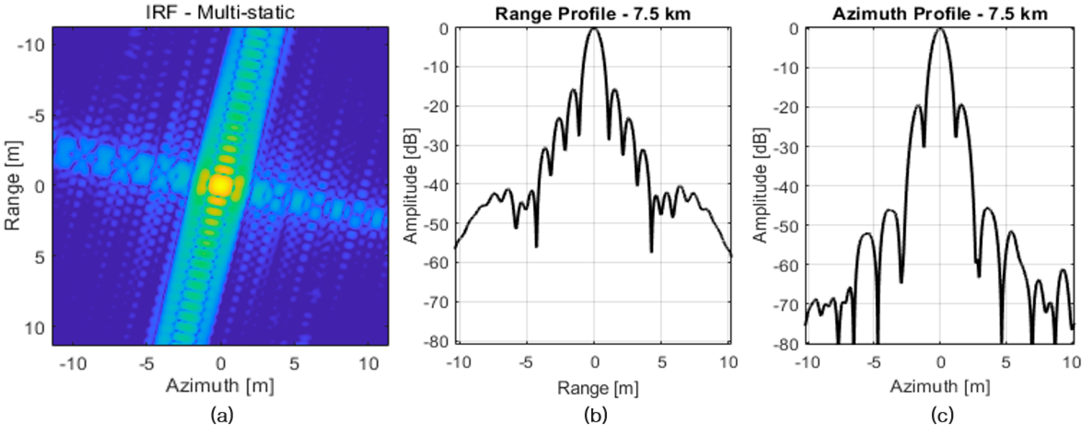
5.1.1. Case of the Designed Orbit Path without Navigation and Attitude Errors
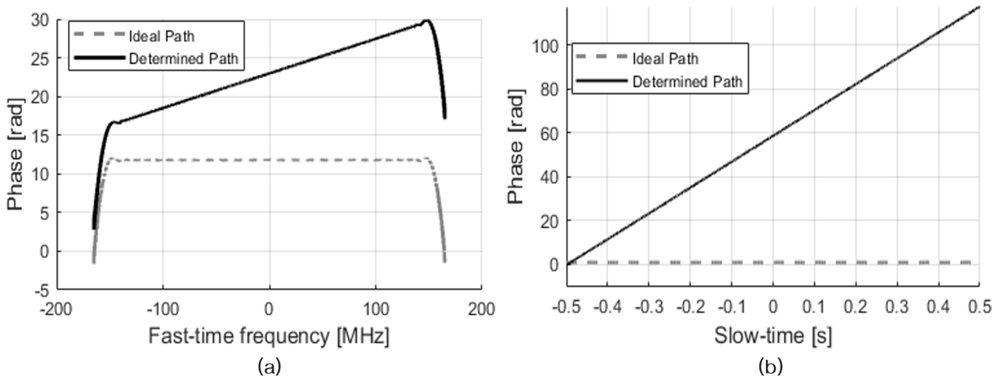
5.1.2. Case of the Determined Orbit Path with Navigation and Attitude Errors
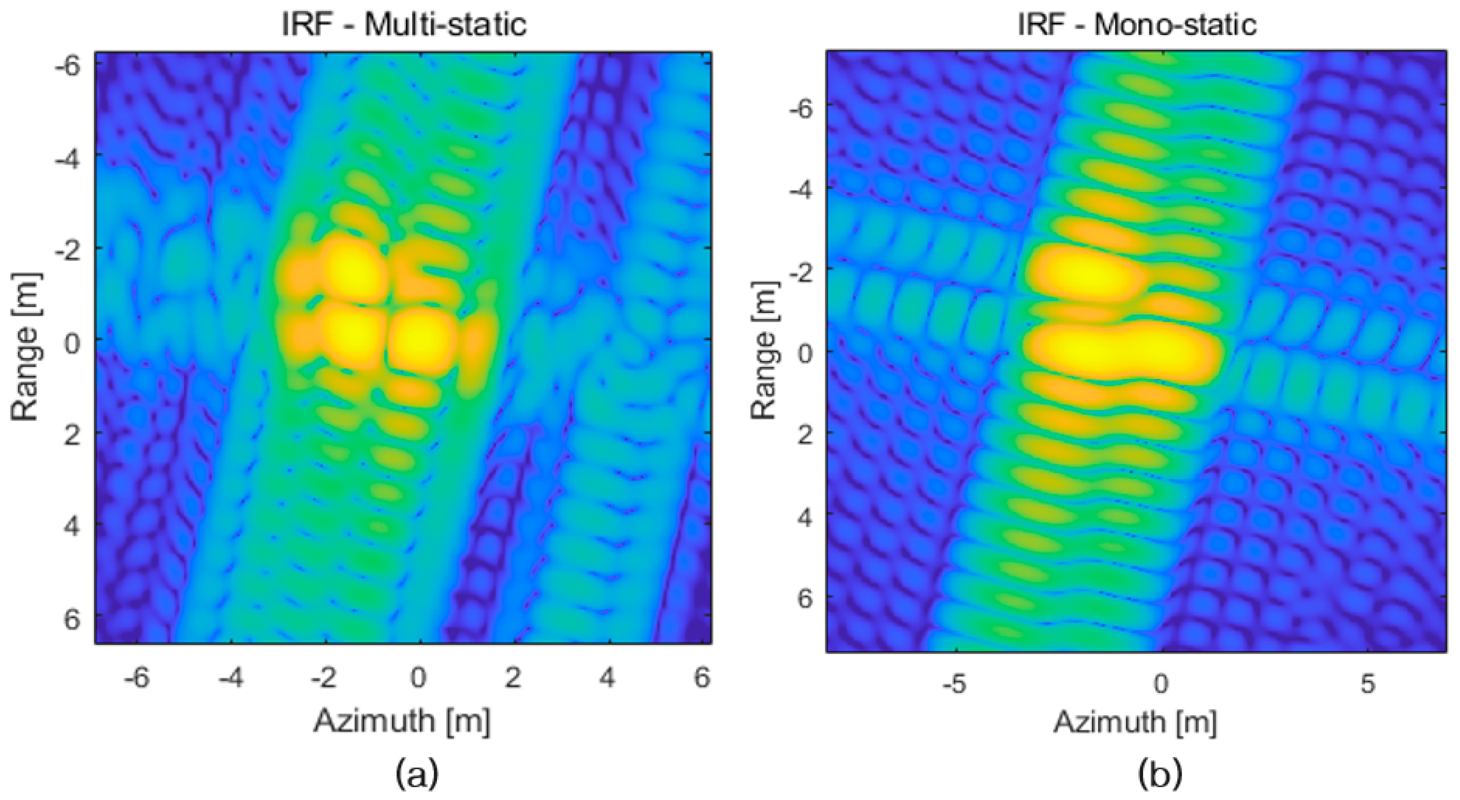
5.1.3. Analysis of the Target Image-Separation Phenomenon Due to Navigation and Attitude Errors
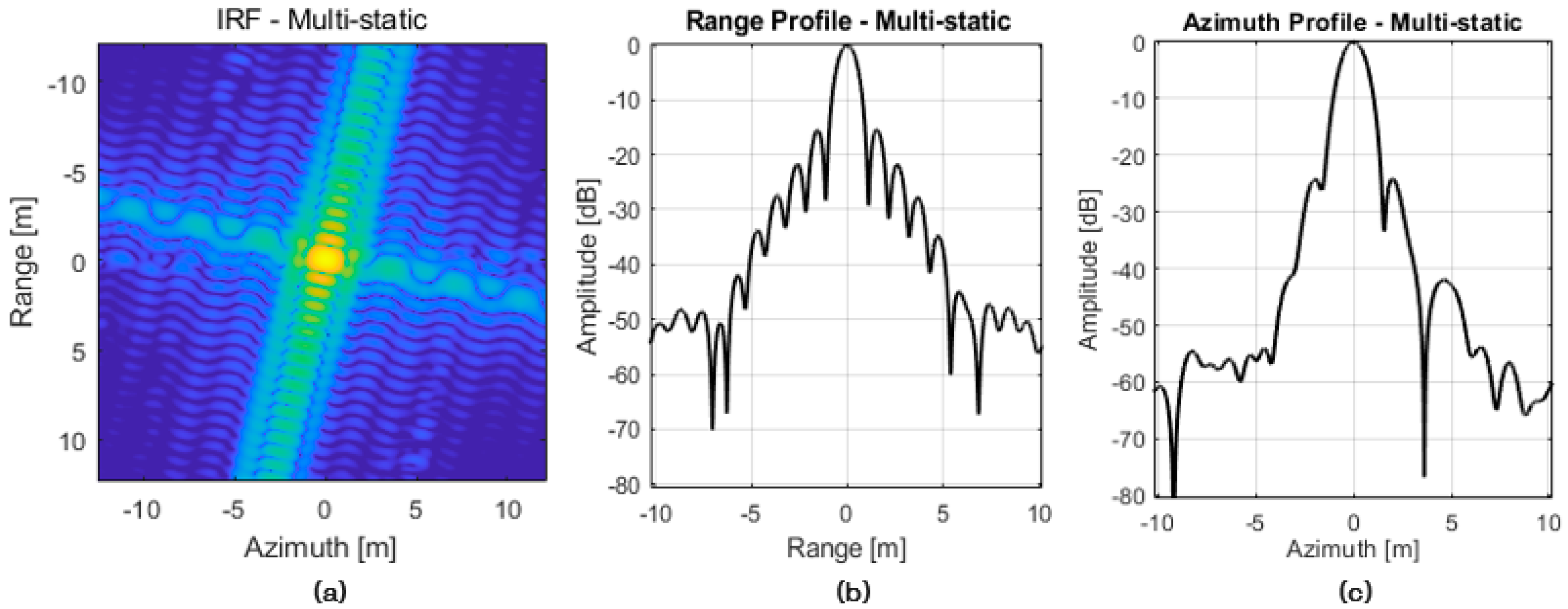
5.1.4. Multistatic SAR Imaging with a Phase-Correction Algorithm under the Determined Orbit Path
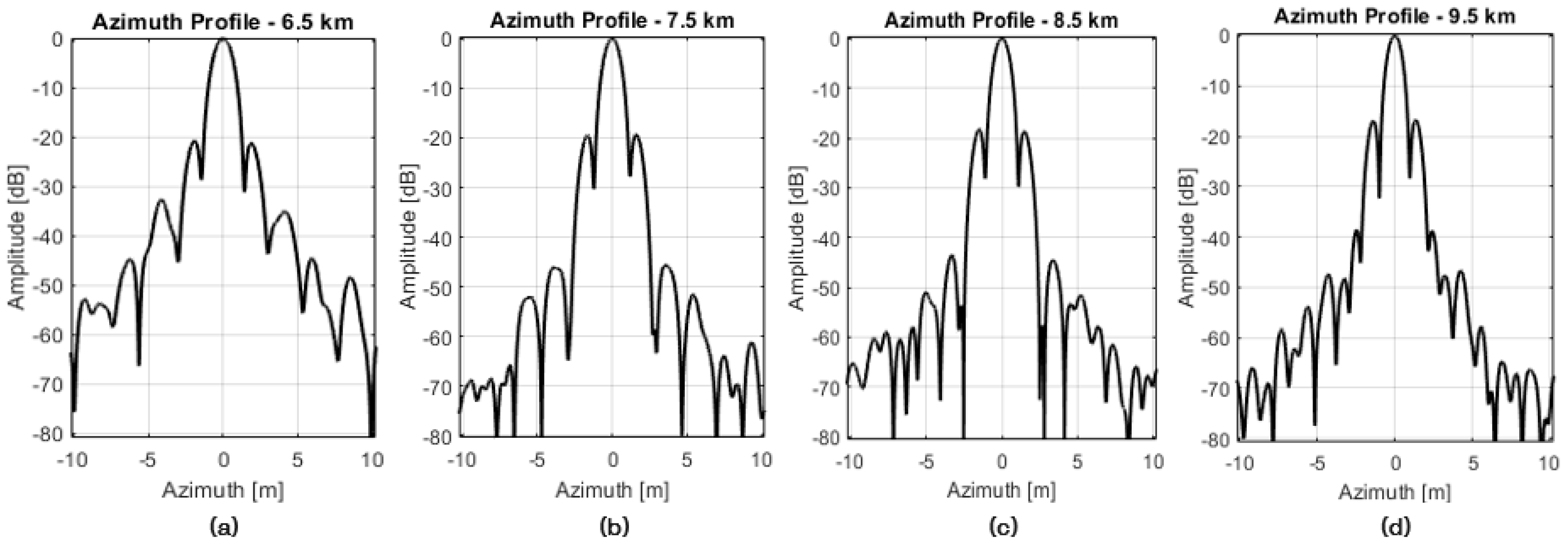
5.2. Design Change of the Multistatic SAR System to Satisfy the Spatial Resolution Requirement
5.3. Analysis of the Multistatic SAR Image with Respect to Navigation and Beam Pointing Errors
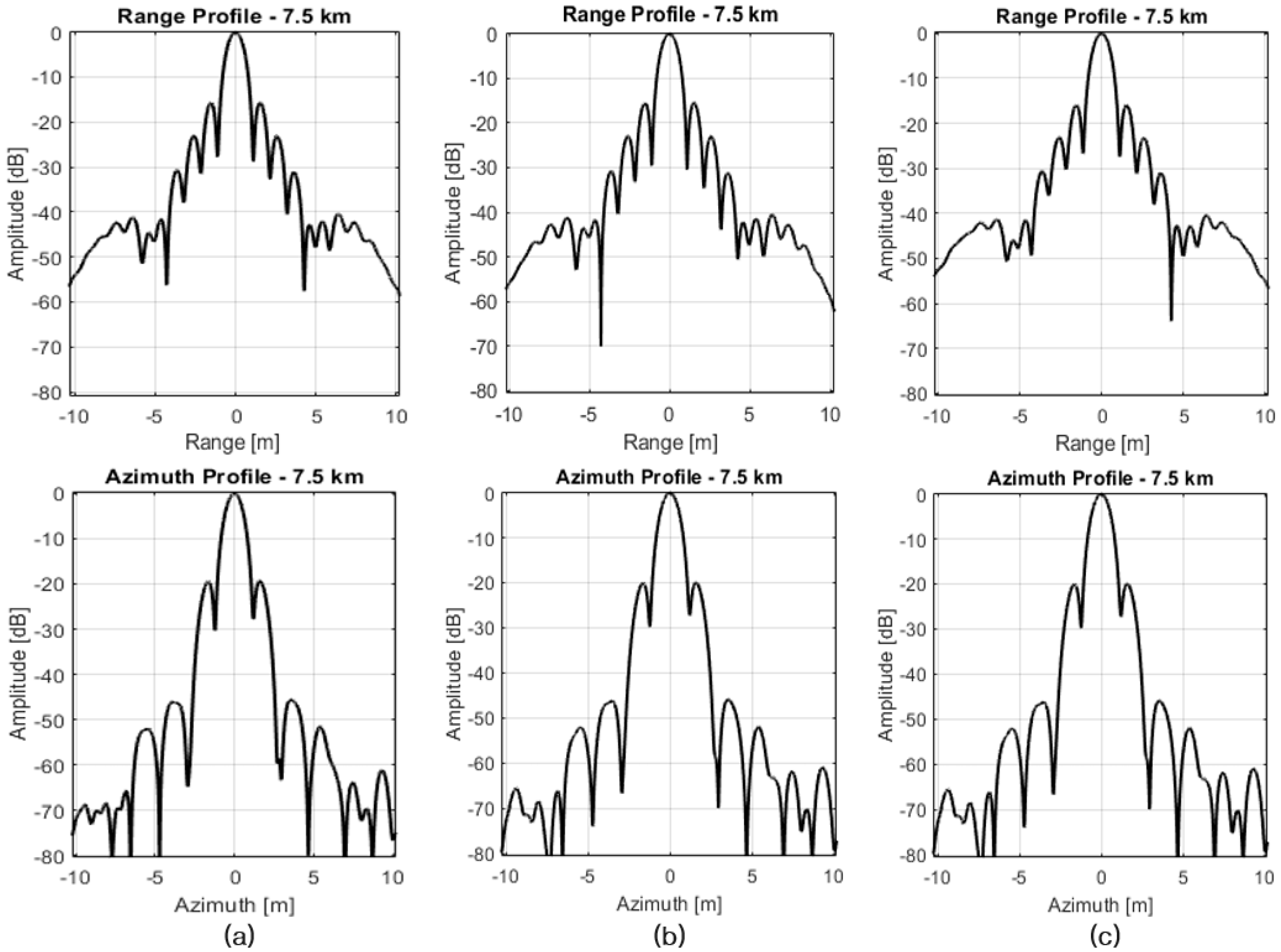
5.3.1. SAR Image Analysis According to the Relative Orbit Determination Error
5.3.2. SAR Image Analysis According to the Relative Orbit Control Error
5.3.3. SAR Image Analysis According to the Absolute Orbit Determination and Attitude Control Errors
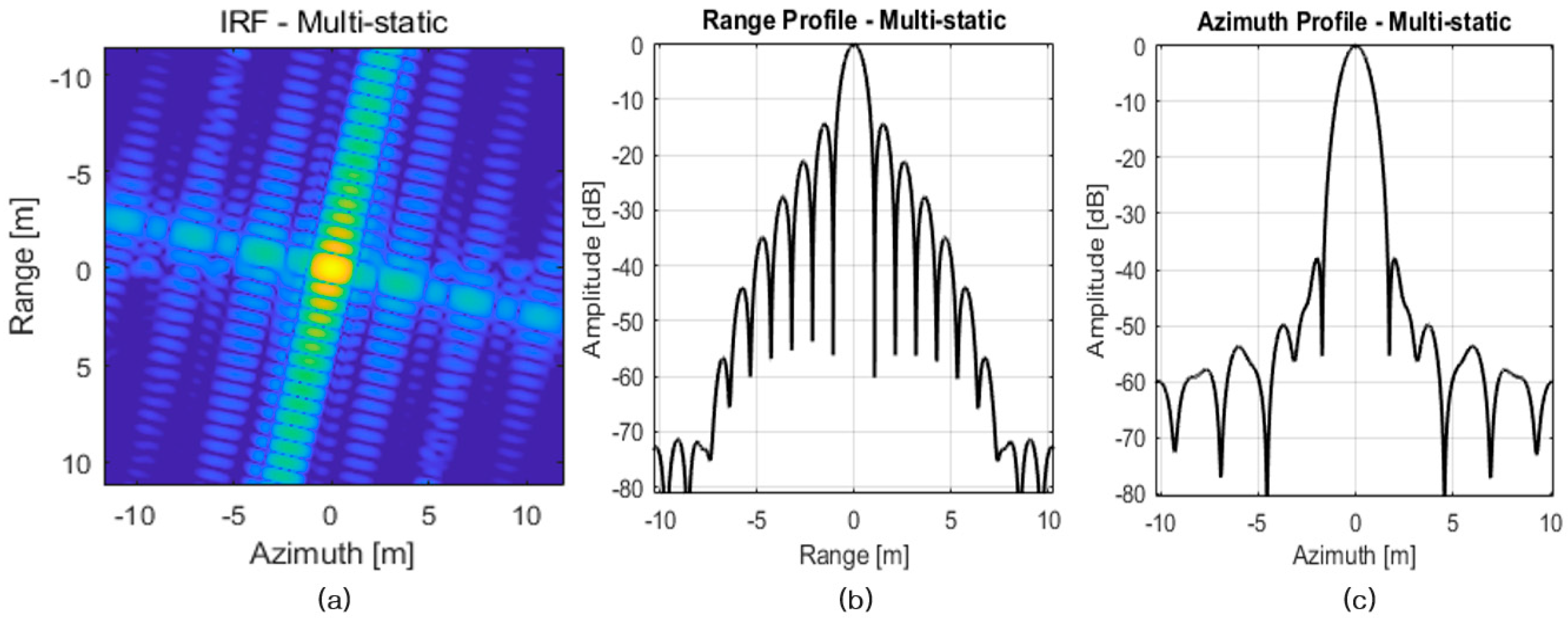
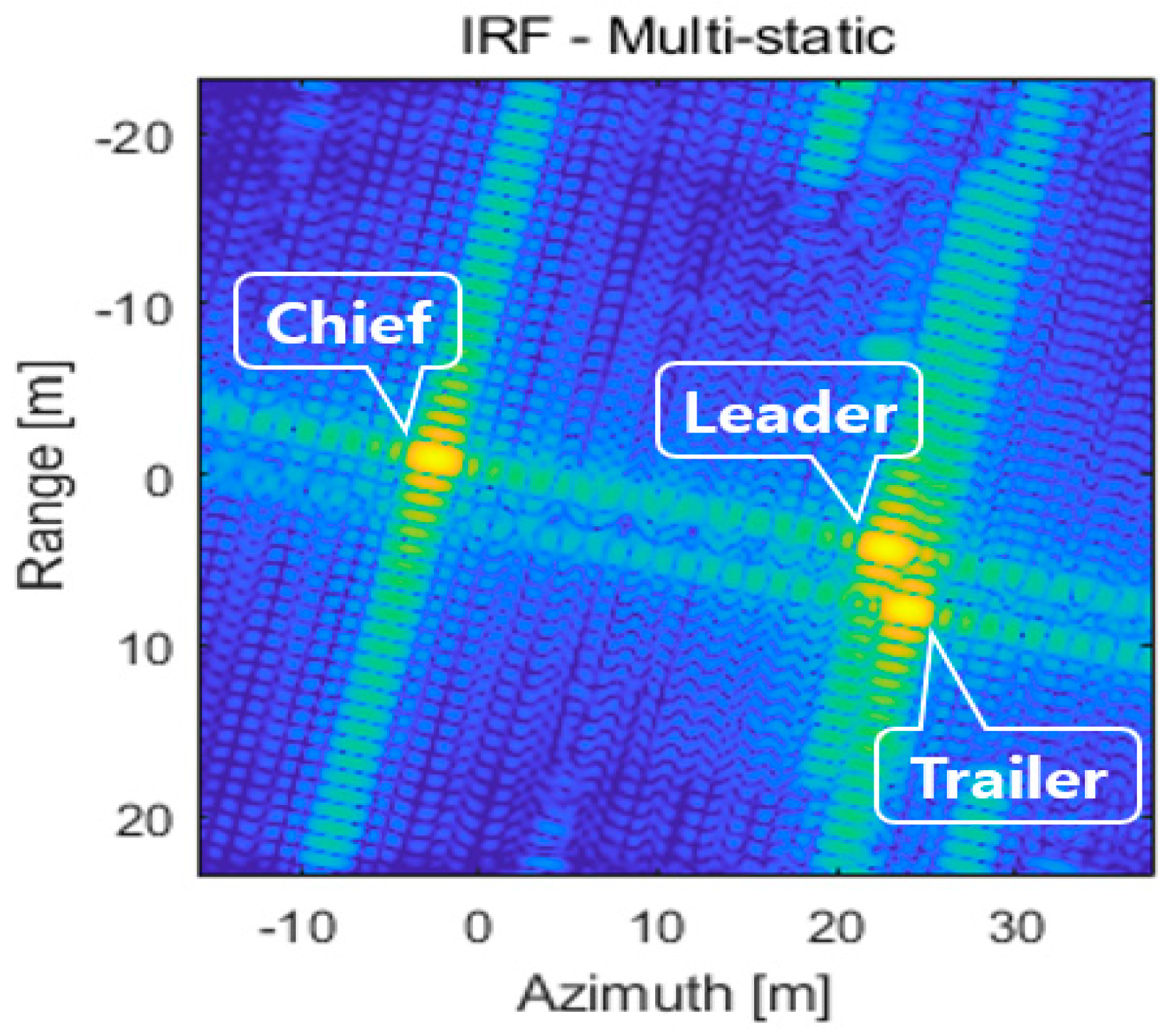
5.4. Performance Verification of the Multistatic SAR System through Near-Multi-Target Imaging Simulation
6. Conclusions
Author Contributions
Funding
Data Availability Statement
Conflicts of Interest
References
- D’Errico, M. Distributed Space Missions for Earth System Monitoring; Springer: Berlin/Heidelberg, Germany, 2013. [Google Scholar]
- Werninghaus, R.; Buckreuss, S. The TerraSAR-X mission and system design. IEEE Trans. Geosci. Remote Sens. 2010, 48, 606–614. [Google Scholar] [CrossRef] [Green Version]
- Naftaly, U.; Levy-Nathansohn, R. Overview of the TECSAR satellite hardware and mosaic mode. IEEE Geosci. Remote Sens. Lett. 2008, 5, 423–426. [Google Scholar] [CrossRef]
- Cumming, I.G.; Wong, F.H. Digital Processing of Synthetic Aperture Radar Data; Artech House: London, UK, 2005. [Google Scholar]
- Castillo, J.; Younis, M.; Krieger, G. A HRWS SAR System Design with Multi-beam Imaging Capabilities. In Proceedings of the 14th European Radar Conference, Nuremberg, Germany, 11–13 October 2017; pp. 179–182. [Google Scholar] [CrossRef]
- Javali, A.; Gupta, J.; Sahoo, A. A review on synthetic aperture radar for earth remote sensing: Challenges and opportunities. In Proceedings of the 2nd International Conference on Electronics and Sustainable Communication Systems (ICESC), Coimbatore, India, 4–6 August 2021; pp. 596–601. [Google Scholar] [CrossRef]
- Wiley, C.A. Synthetic aperture radars-a paradigm for technology evolution. IEEE Trans. Aerosp. Electron. Syst. 1985, 21, 440–443. [Google Scholar] [CrossRef]
- Park, T.Y.; Kim, S.Y.; Yi, D.W.; Jung, H.Y.; Lee, J.E.; Yun, J.H.; Oh, H.U. Thermal design and analysis of unfurlable CFRP skin based parabolic reflector for spaceborne SAR antenna. Int. J. Aeronaut. Space Sci. 2021, 22, 433–444. [Google Scholar] [CrossRef]
- Gens, R.; Van Genderen, J.L. Review article SAR interferometry-issues, techniques, applications. Int. J. Remote Sens. 1996, 17, 1803–1835. [Google Scholar] [CrossRef]
- Heer, C.; Fischer, C.; Schaefer, C. Spaceborne SAR Systems and Technologies. In Proceedings of the 2010 IEEE MTT-S international Microwave Symposium, San Diego, CA, USA, 23–28 May 2010; pp. 538–541. [Google Scholar] [CrossRef]
- Paek, S.W.; Balasubramanian, S.; Kim, S.; de Weck, O. Small-satellite synthetic aperture radar for continuous global biospheric monitoring: A review. Remote Sens. 2020, 12, 2546. [Google Scholar] [CrossRef]
- Grasso, M.; Renga, A.; Fasano, G.; Graziano, M.D.; Grassi, M.; Moccia, A. Design of an end-to-end demonstration mission of a Formation-Flying Synthetic Aperture Radar (FF-SAR) based on microsatellites. Adv. Space Res. 2021, 67, 3909–3923. [Google Scholar] [CrossRef]
- Peral, E.; Im, E.; Wye, L.; Lee, S.; Tanelli, S.; Rahmat-Samii, Y.; Horst, S.; Hoffman, J.; Yun, S.H.; Imken, T.; et al. Radar technologies for earth remote sensing from CubeSat platforms. Proc. IEEE 2018, 106, 404–418. [Google Scholar] [CrossRef]
- Sandau, R.; Roser, H.P.; Valenzuela, A. Small Satellite Missions for Earth Observation: New Developments and Trends; Springer: London, UK, 2010. [Google Scholar]
- Fang, T.; Deng, Y.; Liang, D.; Zhang, L.; Zhang, H.; Fan, H.; Yu, W. Multichannel sliding spotlight SAR imaging: First result of GF-3 satellite. IEEE Trans. Geosci. Remote Sens. 2022, 60, 1–16. [Google Scholar] [CrossRef]
- Tebaldini, S.; Flora, L.; Rocca, F. A Mimo Multi-Static SAR Satellite Formation for High Resolution 3D Imaging at Longer Wavelengths. In Proceedings of the IEEE International Geoscience and Remote Sensing Symposium, Brussels, Belgium, 11–16 July 2021; pp. 1086–1089. [Google Scholar] [CrossRef]
- Seker, I.; Lavalle, M. Tomographic performance of multi-static radar formations: Theory and simulations. Remote Sens. 2021, 13, 737. [Google Scholar] [CrossRef]
- Leng, X.; Ji, K.; Zhou, S.; Xing, X.; Zou, H. An adaptive ship detection scheme for spaceborne SAR imagery. Sensors 2016, 16, 1345. [Google Scholar] [CrossRef] [PubMed] [Green Version]
- Servidia, P.A.; Espana, M. On autonomous reconfiguration of SAR satellite formation flight with continuous control. IEEE Trans. Aerosp. Electron. Syst. 2021, 57, 3861–3873. [Google Scholar] [CrossRef]
- Obata, T.; Arai, M.; Asada, S.; Imaizumi, T.; Suzuki, Y. The autonomous system architecture of the small SAR satellite operation system and on-orbit autonomous operation experiences. In Proceedings of the 35th Annual AIAA/USU Conference on Small Satellites, Logan, UH, USA, 7–12 August 2021. Digital Commons. [Google Scholar]
- D’Amico, S. Autonomous Formation Flying in Low Earth Orbit. Ph.D. Thesis, Delft University of Technology, Delft, The Netherlands, 2015. [Google Scholar]
- Koenig, A.; D’Amico, S.; Lightsey, E.G. Formation Flying Orbit and Control Concept for the VISORS Mission. In Proceedings of the AIAA Scitech 2021 Forum, Virtual Event, 11–15 January 2021; p. 0423. [Google Scholar] [CrossRef]
- Hudson, B. Synthetic Aperture Radar Concept of Operations. UK: OPEN SOURCE SATELLITE. 2021. Available online: https://www.opensourcesatellite.org/ossat-download-synthetic-aperture-radar-concept-operations/ (accessed on 1 August 2022).
- Soleh, M.; Nasution, A.S.; Hidayat, A.; Gunawan, H.; Widipaminto, A. Analysis of antenna specification for very high resolution satellite data acquisition through direct receiving system (DRS). IJReSES 2018, 15, 113–130. [Google Scholar] [CrossRef] [Green Version]
- Singh, J. Spatial Content Understanding of Very High Resolution Synthetic Aperture Radar Images. Ph.D. Thesis, University of Siegen, Siegen, Germany, 2014. [Google Scholar]
- Irvine, J.M. National Imagery Interpretability Rating Scales (NIIRS): Overview and Methodology. In Proceedings of the Optical Science, Engineering and Instrumentation ‘97, San Diego, CA, USA, 27 July–1 August 1997. [Google Scholar] [CrossRef]
- MaCandless Jr, S.W.; Jackson, C.R. Principles of synthetic aperture radar. In Synthetic Aperture Radar Marine User’s Manual; Jackson, C.R., Apel, J.R., Eds.; United States Department of Commerce: Washington, DC, USA, 2004; pp. 1–24. [Google Scholar]
- Dawidowicz, B.; Samczynski, P.; Smolarczyk, M.; Kuzmiuk, M. Analysis of SAR Images Quality Degradation Factors. In Proceedings of the Photonics Applications in Astronomy, Communications, Industry, and High-Energy Physics Experiments IV, Mierzęcice, Poland, 30 May–5 June 2005. [Google Scholar] [CrossRef]
- ICEYE.com. SAR Product Guide; V.4.0. Available online: https://www.iceye-ltd.github.io/product-documentation/5.0/archive/archive/ (accessed on 15 December 2021).
- Saito, H. Compact X Band Synthetic Aperture Radar on 100kg Small Satellite. In Proceedings of the IAA Symposium on Small Satellites for Earth Observation, Berlin, Germany, 20–24 April 2015; pp. 1653–1660, Digital Commons. [Google Scholar] [CrossRef] [Green Version]
- Montenbruck, O.; Kahle, R.; D’Amico, S.; Ardaens, J.S. Navigation and control of the TanDEM-X formation. J. Sci. Astronaut. 2008, 56, 341–357. [Google Scholar] [CrossRef]
- Vallado, D.A.; McClain, W.D. Fundamentals of Astrodynamics and Applications, 4th ed.; Microcosm: Torrance, CA, USA, 2013. [Google Scholar]
- State of the Art Report, Small Spacecraft Technology; Ames Research Center, Small Spacecraft Systems Virtual Institute: Mountain View, CA, USA, 2021.
- Chun, Y.S. Analysis of SAR Image Quality Degradation Due to Pointing and Stability Error of Synthetic Aperture Radar Satellite. Ph.D. Thesis, Chungnam National University, Daejeon, Republic of Korea, 2009. [Google Scholar]
- Larson, W.J.; Werts, J.R. Space Mission Analysis and Design, 3rd ed.; Microcosm: Torrance, CA, USA, 2005. [Google Scholar]
- Scharf, D.P. Analytic yaw-pitch steering for side-looking SAR with numerical roll algorithm for incidence angle. IEEE Trans. Geosci. Remote Sens. 2012, 50, 3587–3594. [Google Scholar] [CrossRef]
- Chobotov, V.A. Spacecraft Attitude Dynamics and Control; Krieger Publishing Company: Malabar, FL, USA, 1991. [Google Scholar]
- Kok, I. Comparison and Analysis of Attitude Control Systems of a Satellite Using Reaction Wheel Actuators. Ph.D. Thesis, Lulea University of Technology, Lulea, Sweden, 2012. [Google Scholar]
- Markley, F.L.; Crassidis, J.L. Fundamentals of Spacecraft Attitude Determination and Control; Springer: New York, NY, USA, 2014. [Google Scholar]
- VECTRONIC aerospace.com. V.S.T. Star Tracker, 68M Performance. Available online: https://www.vectronic-aerospace.com/wp-content/uploads/2020/03/VAS-VST68M-DS2.pdf/ (accessed on 18 August 2022).
- NEWSPACE SYSTEMS.com. Reaction Wheel Performance. Available online: https://www.newspacesystems.com/wp-content/uploads/2022/07/NewSpace-Reaction-Wheel_V11.2.pdf/ (accessed on 18 August 2022).
- Rigling, B.D.; Moses, R.L. Polar format algorithm for bistatic SAR. IEEE Trans. Aerosp. Electron. Syst. 2004, 40, 1147–1159. [Google Scholar] [CrossRef]
- Doerry, A.W. Basics of Polar-Format Algorithm for Processing Synthetic Aperture Radar Images; Sandia National Laboratories (SNL): Livermore, CA, USA, 2012. [Google Scholar]


| Category | Specification |
|---|---|
| Level 3 (2.5~4.5 m) | - Detect individual houses in residential neighborhoods - Identify inland waterways navigable by barges |
| Level 4 (1.2~2.5 m) | - Detect basketball court, tennis court in urban areas - Identify buildings and large ships - Identify individual tracks, rail pairs, control towers |
| Level 5 (0.75~1.2 m) | - Identify tents (larger than two person) at established areas - Identify individual rail cars by type (e.g., gondola, flat, box) - Detect large animals (e.g., elephants, giraffes) in grasslands |
| Contents | Specification |
|---|---|
| Altitude | 570 km |
| Antenna size | 2.2 m 0.5 m |
| Carrier frequency | X-band (9.65 GHz) |
| Incidence angle | 25°~35° |
| Pulse bandwidth () | 400 MHz |
| Pulse repetition frequency (PRF) | 11 kHz |
| Aperture time | 1.4 s |
| Orbital Elements of the Chief Satellite | Relative Orbital Elements of the Deputy Satellite | ||
|---|---|---|---|
| 6378 + 570 km | 0 m | ||
| 0° | −7500 m | ||
| 0.0001 | 0 m | ||
| 0 | 0 m | ||
| 98.19° | 0 m | ||
| 189.89° | 0 m | ||
| Contents | Specifications | |
|---|---|---|
| Dynamic model | Gravity model | JGM-3 60 by 60 |
| Third body perturbation | Sun, Moon, Planets (DE405) | |
| Air drag model | MSISE00 | |
| Solar radiation pressure | Conical spherical model | |
| Parameters for orbit controls | Drag area | 1.0 m2 (chief)/1.5 m2 (deputy) |
| Mass | 100 kg | |
| Orbit determination error | 2 m, 0.02 m/s (1σ) | |
| Relative orbit determination error | 0.1 m, 0.001 m/s (1σ) | |
| direction error | 1° (3σ) | |
| control interval | In-plane: 5 orbit periods Out-of-plane: |
| Minimum | Maximum | |||||||
|---|---|---|---|---|---|---|---|---|
| Ascend/Descend | Ascending | Descending | Ascending | Descending | ||||
| Beam Direction | Left Looking | Right Looking | Left Looking | Right Looking | Left Looking | Right Looking | Left Looking | Right Looking |
| Case No | 1 | 2 | 3 | 4 | 5 | 6 | 7 | 8 |
| Contents | Specifications | |
|---|---|---|
| Satellite | Tensor of inertia | kg·m2 |
| Control rate | 1 Hz | |
| Maximum angular velocity | 2 | |
| Average disturbance torque | 0.001 mN·m (1σ) | |
| Star tracker | Accuracy | 5 arcsec (2σ) |
| Update rate | 5 Hz | |
| Reaction wheel | Maximum torque | 20 mN·m |
| Maximum angular momentum | 0.65 N·m·s | |
| Wheel speed range | ||
| Control accuracy | ||
| Skew angle () | 35° | |
| Rotation angle () | 45° |
| Leader Deputy | Chief | Trailer Deputy | |
|---|---|---|---|
| Total pointing error () | 0.00328° | 0.00332° | 0.00320° |
| Angular velocity error () | 0.00015°/s | 0.00016°/s | 0.00016°/s |
| 6.5 km | 7.5 km | 8.5 km | 9.5 km | |
|---|---|---|---|---|
| Azimuth resolution (m) | 1.125 | 0.962 | 0.891 | 0.815 |
| PSLR (dB) | −20.8 | −19.3 | −18.3 | −16.7 |
Disclaimer/Publisher’s Note: The statements, opinions and data contained in all publications are solely those of the individual author(s) and contributor(s) and not of MDPI and/or the editor(s). MDPI and/or the editor(s) disclaim responsibility for any injury to people or property resulting from any ideas, methods, instructions or products referred to in the content. |
© 2022 by the authors. Licensee MDPI, Basel, Switzerland. This article is an open access article distributed under the terms and conditions of the Creative Commons Attribution (CC BY) license (https://creativecommons.org/licenses/by/4.0/).
Share and Cite
Lee, S.; Park, S.-Y.; Kim, J.; Ka, M.-H.; Song, Y. Mission Design and Orbit-Attitude Control Algorithms Development of Multistatic SAR Satellites for Very-High-Resolution Stripmap Imaging. Aerospace 2023, 10, 33. https://doi.org/10.3390/aerospace10010033
Lee S, Park S-Y, Kim J, Ka M-H, Song Y. Mission Design and Orbit-Attitude Control Algorithms Development of Multistatic SAR Satellites for Very-High-Resolution Stripmap Imaging. Aerospace. 2023; 10(1):33. https://doi.org/10.3390/aerospace10010033
Chicago/Turabian StyleLee, Sangwon, Sang-Young Park, Jeongbae Kim, Min-Ho Ka, and Youngbum Song. 2023. "Mission Design and Orbit-Attitude Control Algorithms Development of Multistatic SAR Satellites for Very-High-Resolution Stripmap Imaging" Aerospace 10, no. 1: 33. https://doi.org/10.3390/aerospace10010033