Article

A Modal-Decay-Based Shock-Capturing Approach for High-Order Flux Reconstruction Method

School of Aeronautic Science and Engineering, Beihang University, Beijing 100191, China
*
Author to whom correspondence should be addressed.
Aerospace 2023, 10(1), 14; https://doi.org/10.3390/aerospace10010014
Submission received: 7 November 2022 / Revised: 11 December 2022 / Accepted: 21 December 2022 / Published: 24 December 2022

Abstract

:
The increasing demand for high-fidelity simulations of compressible turbulence on complex geometries poses a number of challenges for numerical schemes, and plenty of high-order methods have been developed. The high-order methods may encounter spurious oscillations or even blow up for strongly compressible flows, and a number of approaches have been developed, such as slope limiters and artificial viscosity models. In the family of artificial viscosity, which measures smoothness using the modal coefficients, the averaged modal decay (MDA) model employs all of the modes instead of only the highest mode as in the highest modal decay (MDH) model, which tends to underestimate the smoothness. However, the MDA approach requires high-order accuracy (usually P 4 ) to deliver a reliable estimation of smoothness. In this work, an approach used to extend the MDA model to lower orders, such as P 2 and P 3 , referred to as MDAEX, was proposed, where neighboring elements were incorporated to involve more information in the estimation process. A further controlling of the value of artificial viscosity was also introduced. The proposed model was applied to several typical benchmark cases and compared with other typical models. The results show that the MDAEX model recovers the expected accuracy better than the MDA model for P 2 and P 3 and captures flow structures well for shock-dominated flows.

1. Introduction

Currently, there is an increasing demand for high-fidelity simulations of compressible turbulence on complex geometries, which poses a number of challenges for numerical schemes. In this context, an ideal method should be able to achieve high-order accuracy for broadband solutions on unstructured meshes while retaining a good efficiency for modern computer hardware. High-order finite difference methods are well-known for their good accuracy and efficiency, but require block-structured grids of high quality, which is a challenging task for complex geometries [1]. Finite volume methods are naturally adapted for unstructured grids, but require extensive stencils for high-order accuracy [2]. In the last few decades, plenty of high-order methods, including discontinuous Galerkin (DG) [3], spectral difference (SD) [4] and flux reconstruction (FR) [5] or correction procedure via reconstruction (CPR) [6] methods, have been developed.
Despite the superior accuracy with smooth flows, the high-order methods tend to generate spurious oscillations or even blow up for strongly compressible flows. Various methods have been developed to address this issue [7], such as slope limiters, weighted essentially non-oscillatory (WENO) limiters and artificial viscosity models. Slope limiters rely on an indicator to identify troubled cells where the linear mode is limited, and discard components of higher order [8]. A major problem with slope limiters is their detrimental effect on the high-order accuracy [9,10]. For WENO limiters, troubled cells are identified first as well [11]. Instead of limiting the linear mode, WENO reconstruction is conducted for point-wise values or modal coefficients in troubled cells. In [12,13], only cell averages were used for reconstruction, requiring a large stencil for high orders. To relieve this issue, Hermite WENO (HWENO) limiters [14,15,16] were introduced, which use both cell averages and derivatives for reconstruction, reducing the size of the stencil. The rationale behind the HWENO limiter is that more information in the immediate neighborhood is involved, deriving a compact stencil. Zhong et al. [17] and Zhu et al. [18] proposed reconstructing the entire polynomials, i.e., the polynomials on each troubled cell and its immediate neighbors are used directly. The consequent method is compact and accurate. However, it is difficult to extend this method to higher order cases (typically higher than third order) due to the stability issue of extrapolation.
Another promising family of approaches for shock capturing is artificial viscosity models. In the context of finite difference methods, Cook et al. [19,20] proposed an artificial viscosity model based on high-order derivatives of dilation. After that, a number of improvements were made in order to apply the artificial viscosity model for wider use, such as supersonic reacting flows [21] and preparation for large eddy simulation with shocks [22,23]. Furthermore, this strategy was extended to the spectral volume method [24] and DG [25]. Note that computing higher-order derivatives is complex and expensive, especially for unstructured grids. Another strategy is to determine the amount of the added artificial viscosity by the entropy production [26,27]. Furthermore, Chaudhuri et al. [28] extended the method to viscous flows by reducing artificial dissipation in the viscous region. A third approach proposes the use of the decay rate of the modal coefficients to measure smoothness [29]. This method originates from the analogy to the Fourier expansion, i.e., the Pth mode scales as 1 / P 2 for a continuous function. Note that, in [29], only the highest mode was employed to estimate the smoothness, and the smoothness tended to be underestimated. In order to involve more information about the modal decay, an averaged modal decay model is presented to employ all of the modes (except the first mode, which indicates the cell average) to estimate the decay rate [30]. This approach is referred to as the MDA model. However, it has been recognized that modal decay approaches require high-order accuracy (usually P 4 ) to deliver a reliable estimation of smoothness, which limits the scope of the effective application of this approach. For low orders, such as P 2 or P 3 , the MDA model often behaves as overly dissipative.
In this work, we propose an approach used to extend the MDA model to low orders (i.e., P 3 ), where neighboring elements are incorporated to introduce more information on the solutions. Furthermore, artificial viscosity is supposed to scale as O ( h ) around discontinuities, and  O ( h P + 1 ) in smooth regions. Since the MDA model is able to deliver a specific value of the smoothness, the above scaling property is enforced in an explicit manner. The proposed model provides an approach used to apply the MDA model to low orders with a more reliable estimation of smoothness. This paper is organized in the following manner. Section 2 describes the governing equations and the numerical discretization methods used in this paper. Section 3 briefly introduces the modal-decay-based discontinuity sensor, including the MDH model, the MDA model and the extension of the MDA model to lower orders. Section 4 shows several benchmark test cases to demonstrate the performance of the propose method, followed by some conclusions in Section 5.

2. Numerical Methods

2.1. Governing Equations

The conservation law is given as
q t + · f · g = 0 ,
where q is the state variables, f is the convective flux and  g is the viscous flux. In this paper, g provides artificial diffusion for the purpose of stabilizing shocks, and takes the Laplacian form given by
g = μ w , w = q ,
where μ is the coefficient of artificial viscosity, which will be described in more detail below.

2.2. Flux Reconstruction Method

The conservation law is discretized by the high-order flux reconstruction (FR) scheme. Considering a one-dimensional case for simplicity, first, the computational domain Ω is divided into non-overlapping elements Ω h . A degree P polynomial defined on a set of N = P + 1 points (solution points, SPs) is used to represent the solution and the flux in the element. In this paper, the SPs were located at the Legendre–Gauss points. By adopting N p solution points, the 1-D Lagrange basis polynomial of N p 1 degree is
l i ( x ) = j = 1 , j i N p x x j x i x j , i = 1 , . . . , N p .
Once given the values at the SPs, the solution q in the element Ω h is approximated by q h , which is defined by:
q h ( x ) = i = 1 N p q h ( x i ) · l i ( x ) ,
where q h ( x i ) is the value of the solution at SP located by x i . The flux polynomial f ( x ) of order P can be expressed in a similar manner. Note that q h ( x ) and f ( x ) are both Pth-order piece-wise continuous polynomials and might not be continuous across the interfaces between the elements. The solution polynomial is then extrapolated to the interfaces, forming left and right interface states q L and q R on each element. Then, the common numerical flux f * can be calculated from f ( q L ) and f ( q R ) on the interface via an approximate Riemann solver such as the Roe method [31] for the inviscid flux and the CDG [32] method for the viscous flux.
In the FR approach, the discontinuous polynomial of flux is then made continuous by introducing correction functions, which are given by:
Δ f ( x ) = [ f L * f ( 1 ) ] g L ( x ) + [ f R * f ( 1 ) ] g R ( x ) ,
where f L * and f R * denote the common interface fluxes on left and right interfaces, f ( 1 ) and f ( 1 ) are extrapolated states of the flux polynomial f ( x ) on left and right interfaces and g L ( x ) and g R ( x ) are left and right correction functions that are order P + 1 polynomials and satisfy boundary conditions:
g L ( 1 ) = 1 , g L ( 1 ) = 0 ,
g R ( 1 ) = 0 , g R ( 1 ) = 1 .
Then the corrected continuous flux f C is given by
f C ( x ) = f ( x ) + Δ f ( x ) .
Finally, the divergence of the continuous flux is calculated at the solution points to update the solution. In this paper, the left and right Radau polynomials were chosen as correction functions g L and g R , respectively, which recover the standard DG scheme [5]. The strong stability preserving five-stage fourth-order Runge–Kutta (SSPRK54) [33] was adopted for explicit time integration in the numerical experiments in this paper.

3. Shock-Capturing Model

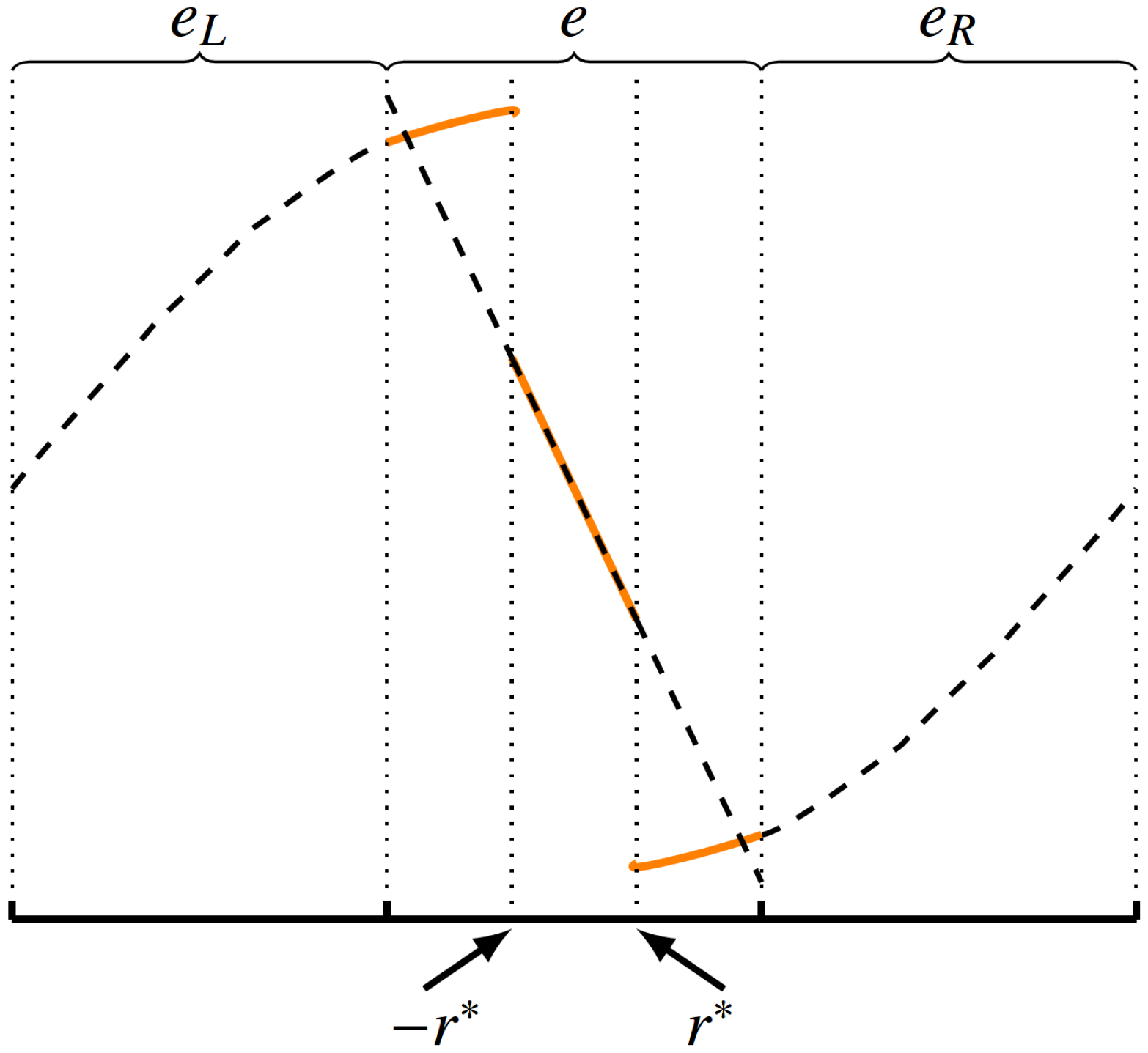
3.1. Modal-Decay-Based Discontinuity Sensor

To help understand the mechanism of the modal-decay-based discontinuity sensor, the continuous Fourier expansion of q ( r ) , r [ 1 , 1 ] is introduced as
q h ( r ) = m = N N q ¨ m exp ( i π m r ) ,
If q ( r ) C τ and is periodic, we have [7]
| q ¨ m | 1 m τ + 1 , | q ¨ m ( n ) | 1 m τ + 1 n .
In [29], a modal decay model was proposed to relate the strength of the discontinuity to the decay rate of the modal expansion coefficients. For this model, a truncated solution is first introduced as
q ˜ h = m = 0 N P 1 1 q ^ m φ m .
Then, the discontinuity sensor is defined as the energy fraction contained in the highest mode, i.e.,
S = q h q ˜ h L 2 2 q h L 2 2 ,
where · L 2 denotes the standard L 2 norm on element K. By invoking an analogy to the Fourier expansion, S should scale as 1 / P 4 if  q ( r ) C 1 and φ m is orthonormal. In principle, artificial viscosity is required when S > 1 / P 4 . This model is referred to as the highest modal decay (MDH) model due to its dependence on the highest mode only.
The MDH model shows, in a qualitative manner, how a large value of the sensor S indicates that a problem exists. However, it is still difficult to identify an accurate scaling with only the highest mode given the oscillatory modal coefficients [7] and the insufficient information. As a result, the MDH model often underestimates the smoothness. To overcome this issue, more information in the modal expansion should be used to determine the decay rate more accurately. This is the motivation behind the model proposed by Klöckner et al. [30].
In order to illustrate the idea, we return to the Fourier case again. Equation (10) is attributed to the following relation:
d d x exp ( i n x ) x ( π , π ) L m = n exp ( i n x ) x ( π , π ) L m , for m [ 1 , ) .
A polynomial analogy is also available, given as
d d r φ m r ( 1 , 1 ) L 2 3 n 2 φ m r ( 1 , 1 ) L 2 .
Therefore, we first assume that the modal coefficients scale as
| q ^ m | C m τ .
Taking the logarithm on both sides of Equation (15), we have
l o g | q ^ m | l o g ( C ) τ l o g ( m ) .
The decay rate τ is computed in a least-squared manner from the following problem:
m = 1 N P 1 ( l o g | q ^ m | ( l o g ( C ) τ l o g ( m ) ) ) 2 .
Note that the cell average is not included when determining the decay rate by Equation (17). Therefore, when the solution is constant with slight oscillations, the sensor would sense the oscillations and yield a decay rate of nearly zero. This is clearly undesirable as it would produce an overly large dissipation. To address this issue, a baseline modal decay needs to be introduced. Furthermore, the estimation method assumes that the modal coefficients decay monotonously, which is usually not the case. A skyline procedure is required to fix this. The detailed algorithm can be found in Algorithm 1. Since the smoothness is measured in an averaged sense, the model is called the averaged modal decay (MDA) model. The expected decay rate τ for different situations is given as
τ = 1 , q is discontinuous , 2 , q C 0 \ C 1 , 3 , q C 1 \ C 2 .
Algorithm 1: Discontinuity sensor of MDA
 1:  function S e n s o r M D A ( q h ( r , t ) )
 2:  Fix with baseline modal decay:
 3:  Construct a perfect modal decay as:
   b m = m P m = 1 N P 1 m 2 P , m = 1 , , N P 1 .
 4:  Modify the modal coefficients q ^ m as:
   | q ^ m | 2 | q ^ m | 2 + q h L K 2 2 | b m | 2 , m = 1 , , N P 1 .
 5:  Fix with skyline procedure:
 6:  Ensure the modal coefficients q ^ m to be monotone as:
     q ^ m max n = m i n ( m , N P 2 ) , , N P 1 | q ^ n | , m = 1 , 2 , , N P 1 .
 7:  Least-squared procedure:
 8:  Compute the decay rate τ in a least-squared manner from the following problem:
     m = 1 N P 1 ( l o g | q ^ m | ( l o g ( C ) τ l o g ( m ) ) ) 2 .
 9:  return τ
 10: end function

3.2. Extension to Arbitrary Orders

The MDA sensor relies on the available information in the polynomial expansion. Therefore, when the polynomial order is low, the estimation procedure tends to be inaccurate. For example, when the solution is nearly constant, the decay rate is close to P, where the smoothness tends to be underestimated for P < 4 . In order to improve the accuracy of the estimated decay rate, information from the neighboring cells should be involved.
Assume that the approximate solutions for the current element and its left and right neighbors are denoted as q h ( r , t ) , q L ( r , t ) and q R ( r , t ) , respectively. Then, we have
q e x ( r , t ) = γ L q L ( r , t ) + γ q h ( r , t ) + γ R q R ( r , t ) ,
where the weighted coefficients γ L , γ , γ R are given as
γ L = 1 , r r * . 0 , r > r * . γ R = 1 , r r * . 0 , r < r * . γ = 1 γ L γ R ,
where r * = 2 ( P * 1 ) 3 ( P m a x 1 ) + 1 3 , P * = m i n ( P m a x , P + 1 ) , P m a x = 5 . This means that r * | P = 1 = 0.5 , r * | P 4 = 1 .
The new modal coefficients of q e x are obtained by projection as
q e x ( r , t ) = m = 0 P e x q ^ m e x φ m ( r ) ,
and scale as
| q ^ m e x | C m τ .
To evaluate the smoothness, the extended polynomial q e x ( r , t ) is fed into Algorithm 1 instead. Note that P denotes the polynomial order for q h ( r , t ) , q L ( r , t ) and q R ( r , t ) , whereas P e x denotes the polynomial order for q e x ( r , t ) . An example of the extended MDA sensor is shown in Figure 1, which indicates a discontinuity in the original solution of the current element e for low polynomial orders P (typically P 3 ). In such cases, τ is close to P indicating moderate non-smoothness using the original MDA model. With the extended MDA sensor, the discontinuity is steepened artificially and thus detected correctly with a large enough P e x .

3.3. Localized Nonlinear Viscosity

The scaling of the artificial viscosity in [29,30] is of O ( h ) as long as the model is activated, which tends to cause excessive dissipation for small fluctuations and destroy the high-order accuracy. Therefore, it is essential for us to further decrease the artificial dissipation where the sensor is switched off. The viscosity is proposed here to be computed as
μ = μ m a x 1 , if τ < τ 0 , h P ( τ τ 0 ) τ 1 τ 0 , if τ 0 τ τ 1 , 0 , otherwise .
and μ m a x is given by
μ m a x = c m a x ( h / P ) max x G K | f ( q h ( x , t ) ) | .
This can ensure that the viscosity is O ( h ) around shocks, and approaches O ( h P + 1 ) when the flow turns smooth. Theoretically, τ 0 = 1 , whereas, in practice, τ 0 is chosen within [ 1 , τ 1 ) to enhance robustness. In this paper, τ 1 was fixed to 3.

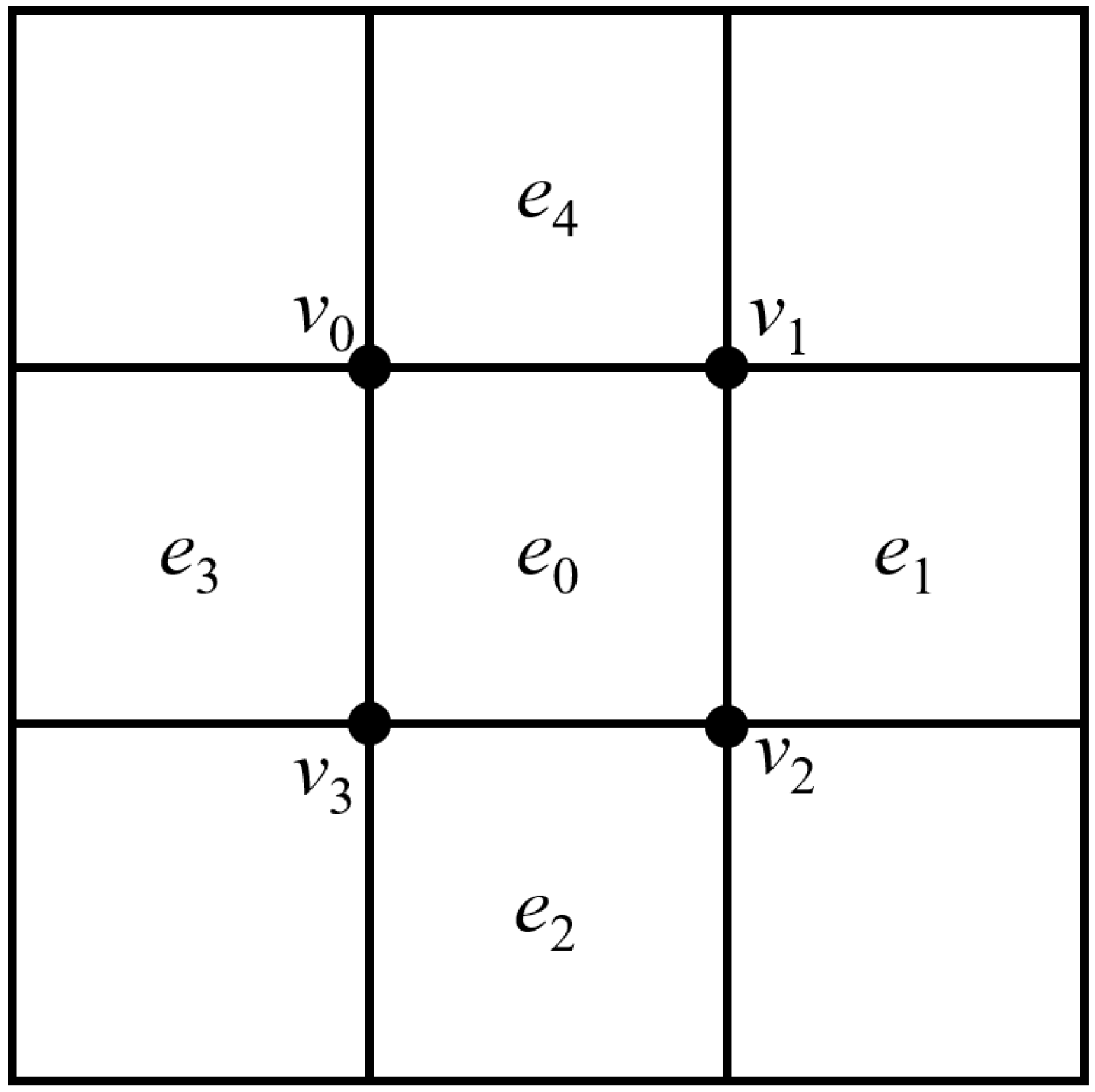
3.4. Multi-Dimensional Case

In this section, we propose a simple yet effective way to extend the above one-dimensional model to multi-dimensional cases. The idea is illustrated in the two-dimensional case and its extension to three-dimensions is straight-forward.
The extension to a 2D case is described (see Figure 2) as the following:
  • Step 1. Extrapolate the polynomials q 1 , q 2 , q 3 , q 4 of the four neighboring elements ( e 1 , e 2 , e 3 , e 4 ) onto the current element e 0 .
  • Step 2. Estimate a decay rate along each face of the current element using the one-dimensional approach. Take face ν 0 ν 1 as an example. The extrapolated q 1 , q 3 are reduced to this face to serve as the two neighboring solutions q L , q R in the 1D case. The same approach is applied to the remaining faces.
  • Step 3. Choose the smallest one of all of the decay rates to be the decay rate of the element e 0 .
  • Step 4. Compute the viscosity using Equation (23).
Remark 1.
In the above extension method, only q 1 , q 3 are employed to form the neighboring solutions for face ν 0 ν 1 . We note that this choice is not unique, and other approaches are also possible.

4. Numerical Results

In the following, we tested the performance of the proposed method using both smooth and non-smooth cases. The results were compared with other models, including MDH, MDA and the dilation-based (DB) model [34]. Note that the proposed method was termed as MDAEX in this work.

4.1. Convergence Tests with Smooth Problems

4.1.1. One-Dimensional Linear Transport

In this section, the one-dimensional linear transport case was conducted to test the accuracy of the proposed model for the smooth flow. The computational domain is [0, 2] and the exact solution is q ( x , t ) = s i n ( π ( x t ) ) . The numerical error is evaluated at t = 4.0 . The results are given in Table 1 and compared with typical artificial viscosity models, as well as the linear cases where no shock capturing is applied. Note that a super-convergent ( 2 P + 1 )th order of accuracy can be observed for P 1 and P 2 in linear cases. It can be observed that the original MDA model achieves a comparable accuracy only when the polynomial order is higher than P 3 . The MDAEX model, on the other hand, recovers the same accuracy to the linear case away from coarse resolution.

4.1.2. Two-Dimensional Isentropic Vortex Convection

The accuracy of the proposed method was further examined with the two-dimensional isentropic vortex convection in this section. The computational domain is [ 10 , 10 ] × [ 10 , 10 ] with periodic boundary conditions. The center of the initial vortex was set at ( x 0 , y 0 ) = ( 0 , 0 ) and the vortex was convected for one period. The initial field is given following the procedures in [35], which avoid the interruption of initial oscillation led by periodic conditions. The results are given in Table 2, where the number N stands for the number of cells along each edge. As can be seen, the results are similar to those in the one-dimensional case. MDAEX is able to recover the expected accuracy for all cases given a sufficient resolution, behaving superior to its counterpart MDA.

4.2. Shock-Dominated Problems
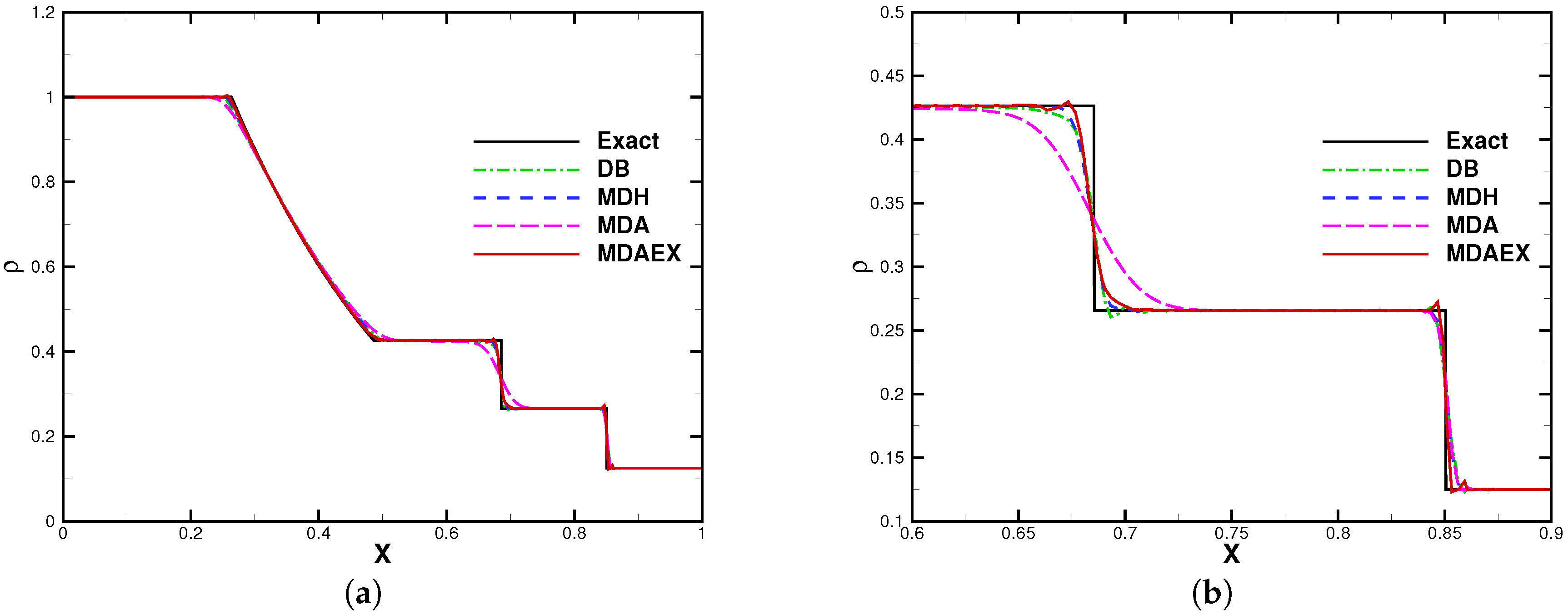
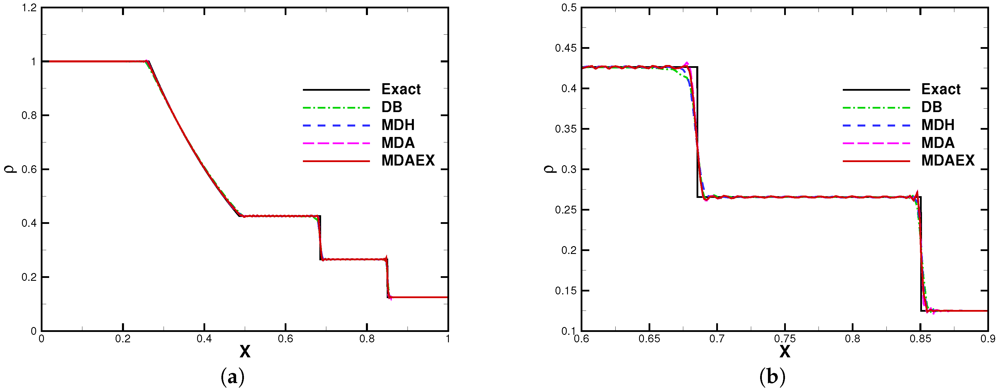
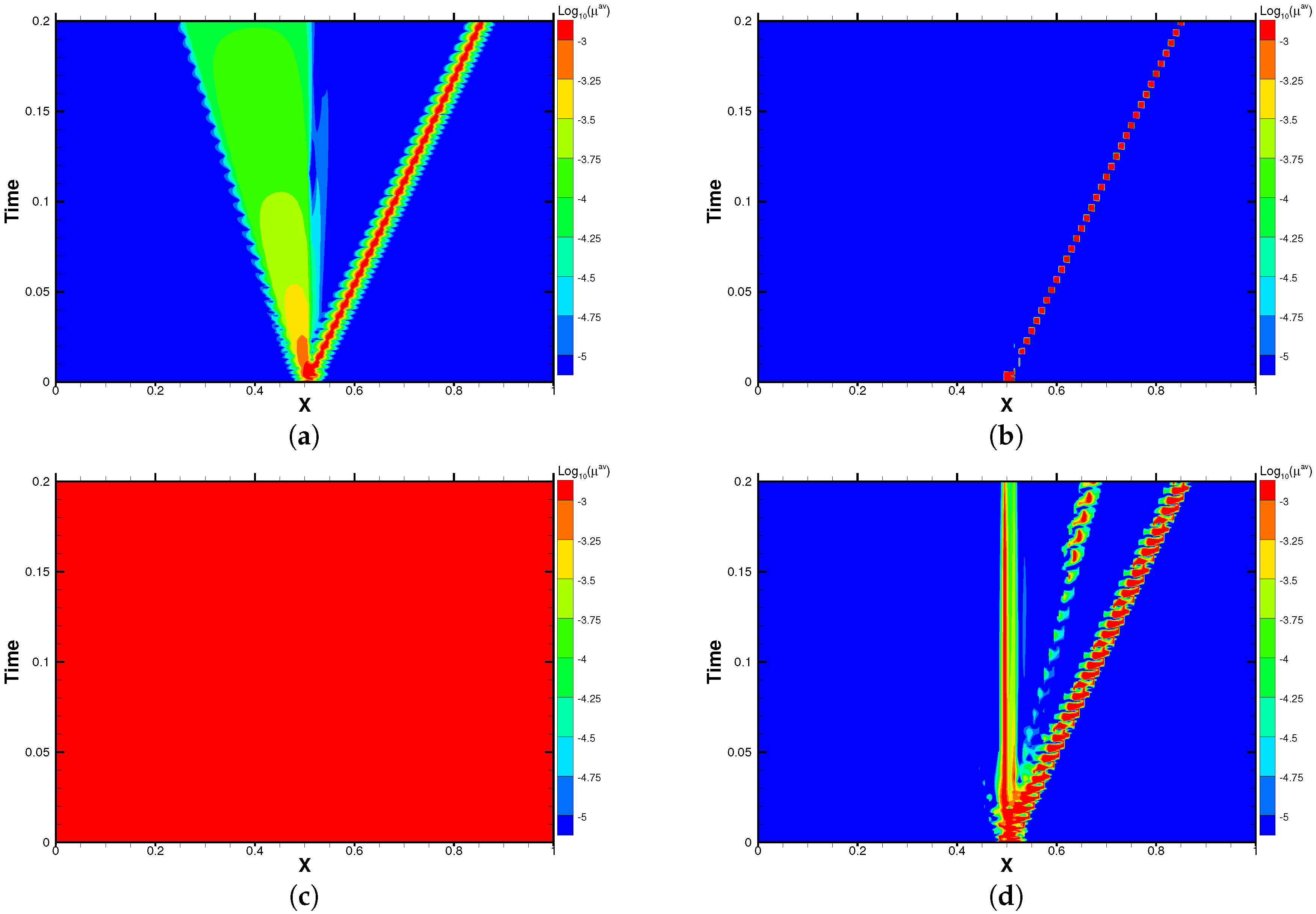
4.2.1. Sod Problem

The computational domain of the Sod problem was chosen to be [ 0 , 1 ] discretized with 100 uniform elements. The initial domain is given by
( ρ , u , p ) = ( 1 , 0 , 1 ) , x < 0.5 , ( 0.125 , 0 , 0.1 ) , x > 0.5 .
To compare dissipative features of aforementioned models, the density profiles at t = 0.2 are presented in Figure 3, Figure 4, Figure 5 and Figure 6, which show that MDAEX is able to produce reasonable results for all accuracy orders despite slight oscillations. The development of artificial viscosity for P 2 is compared in Figure 7, where the difference is more noticeable. At this polynomial order, MDA is completely unable to identify different structures. Furthermore, DB is very dissipative whereas MDH is not dissipative enough. The dissipation of MDAEX is somewhere between DB and MDH. Note that, though MDAEX pollutes less of the region than DB, the max viscosity is larger, which helps to explain the slightly more dissipative result in Figure 4. We believe that the feature of controlling viscosity distribution is more important since the maximum viscosity can be adjusted by empirical parameters. This feature may be profitable in the simulation of more complex flows, which should be conducted in future work.

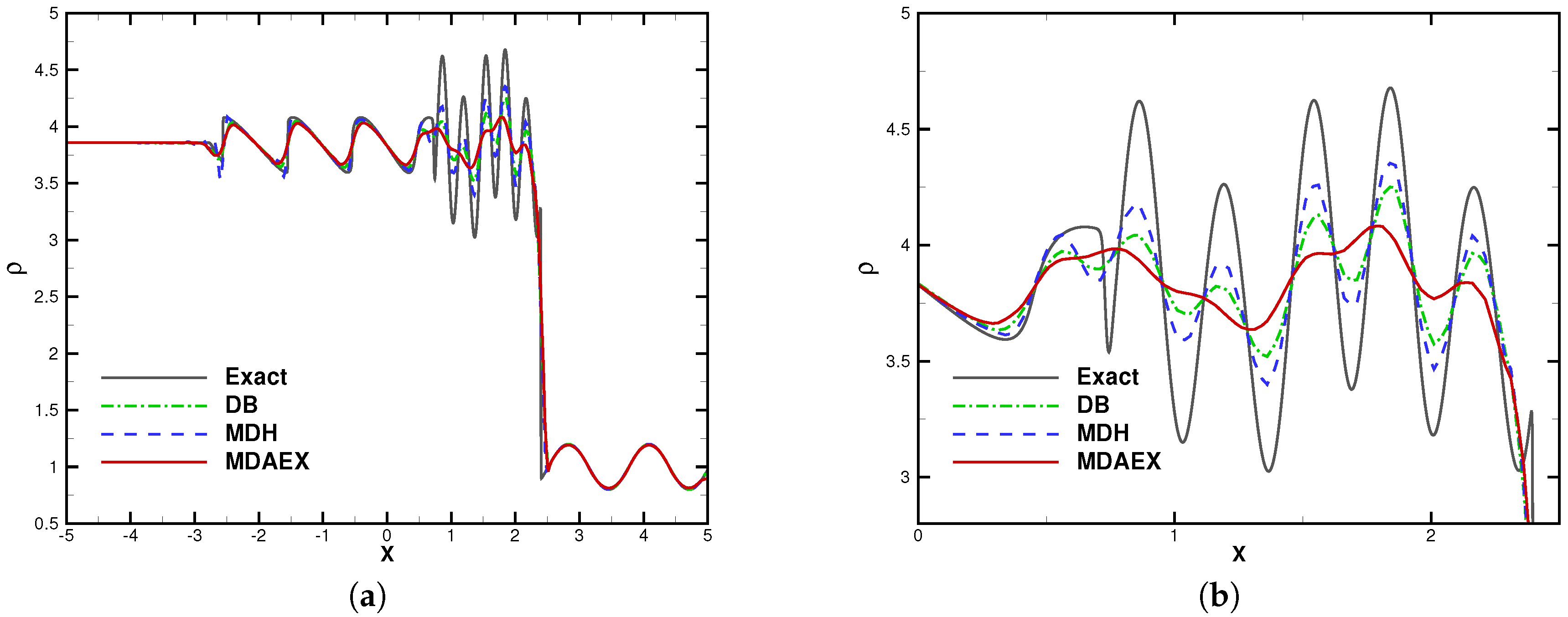
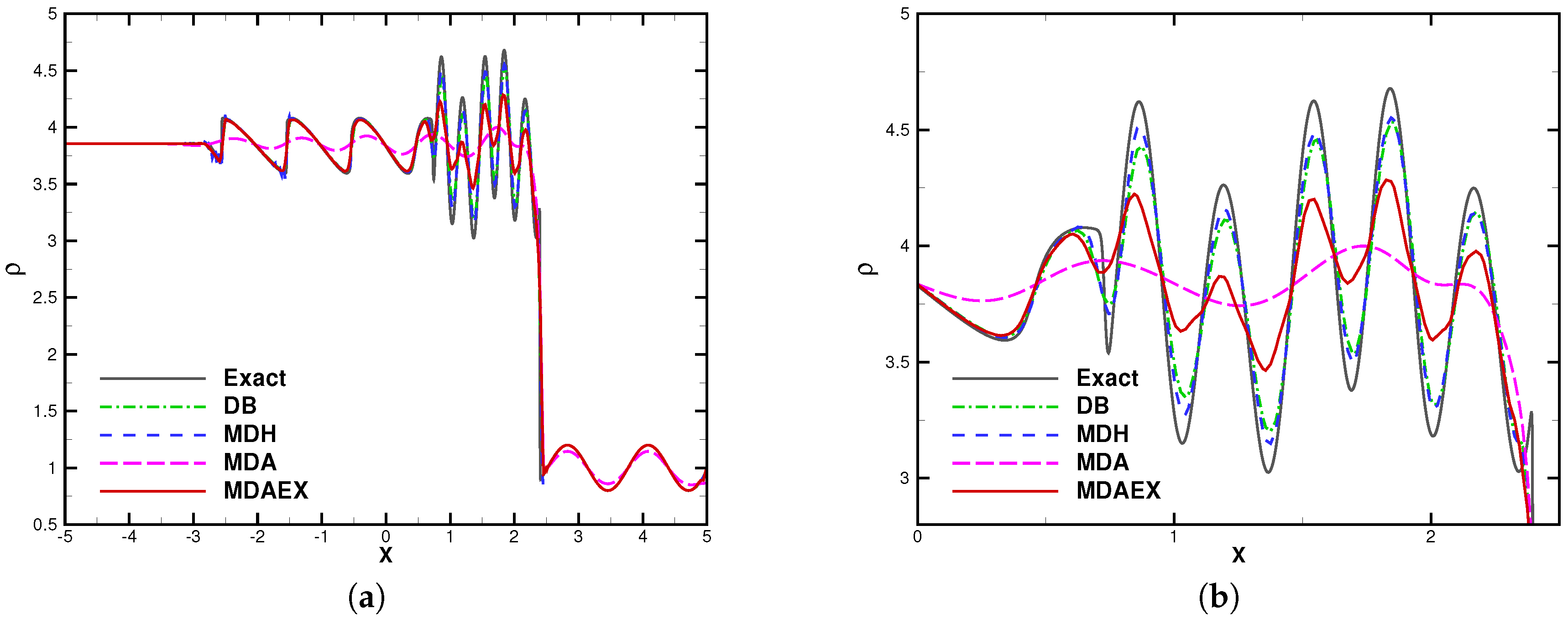
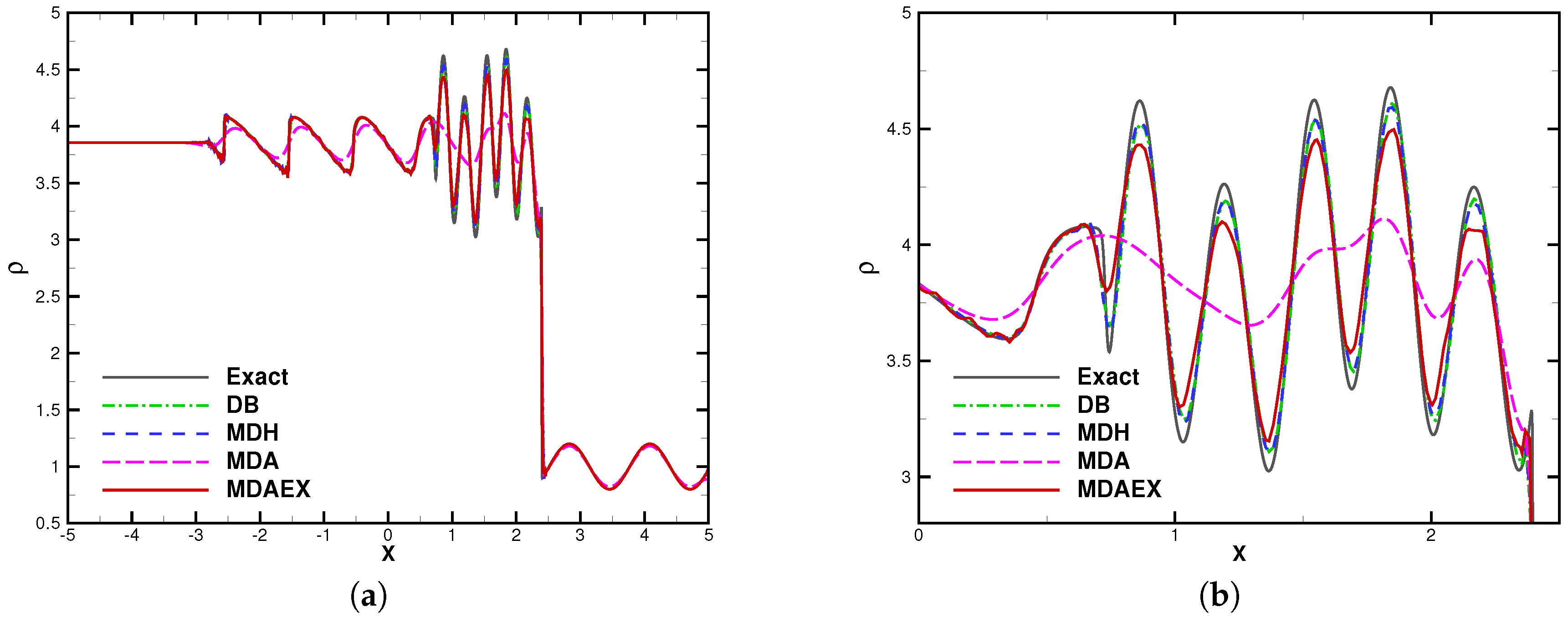
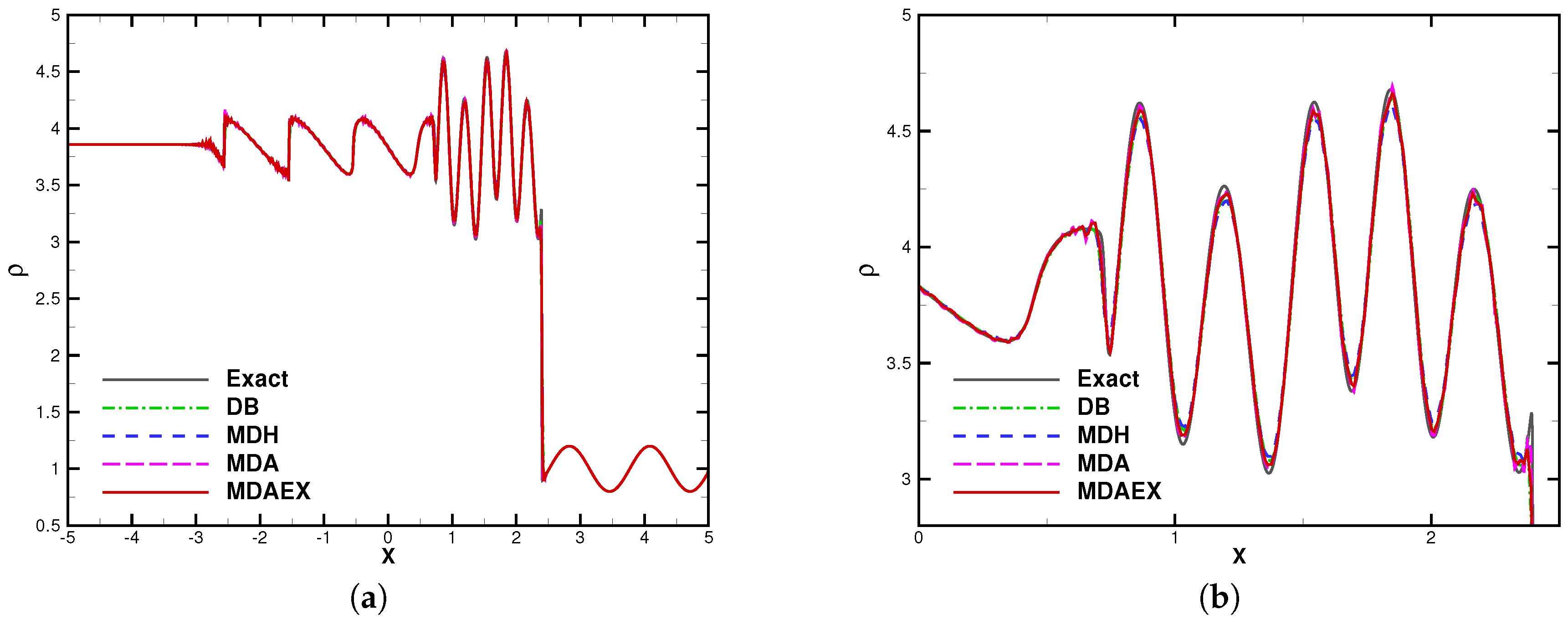
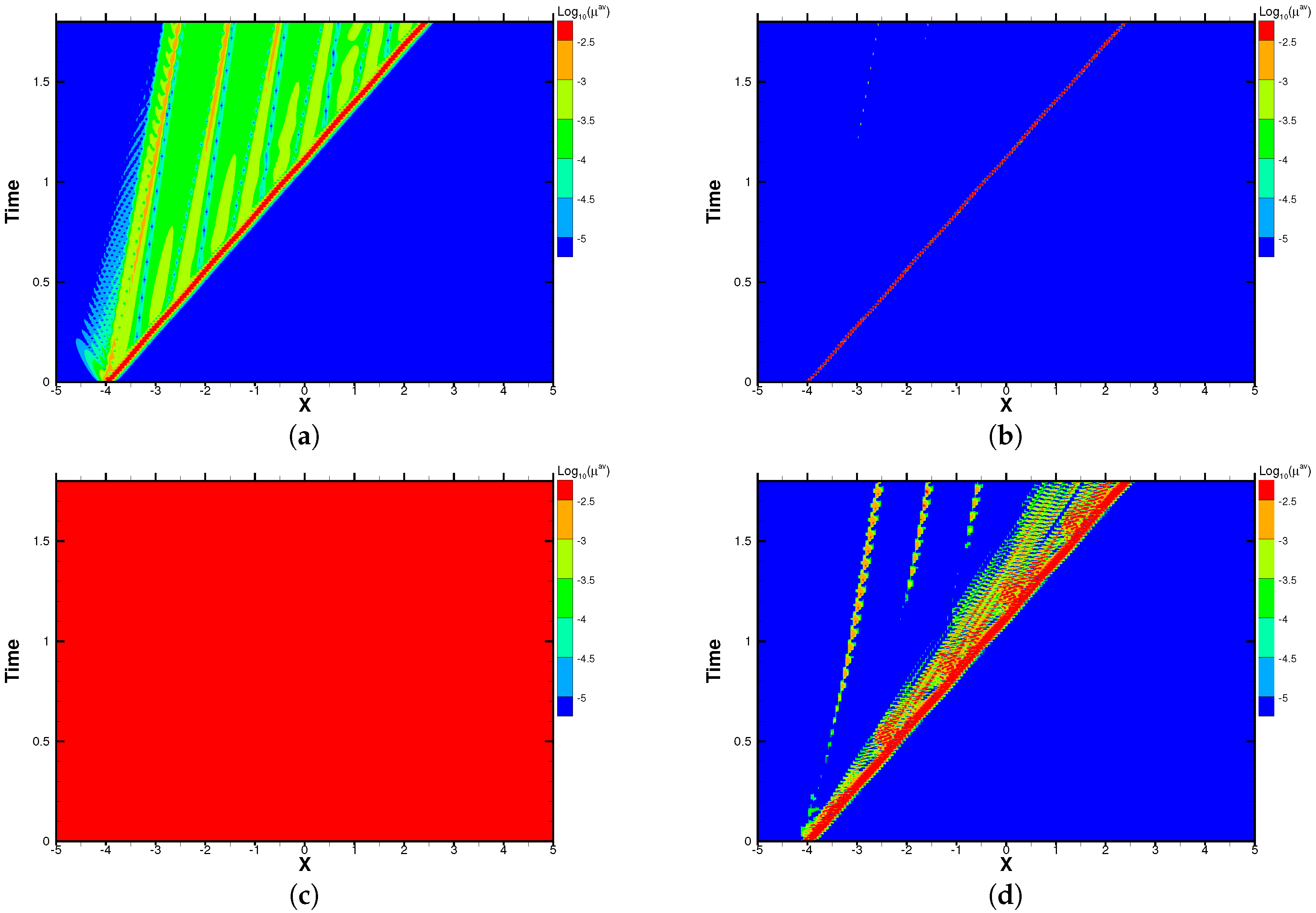
4.2.2. Shu–Osher Problem

The Shu–Osher problem is considered as a one-dimensional model of a shock/turbulence interaction, including shocklets and fluctuations simultaneously. Consequently, shock-capturing methods are required to suppress oscillations without causing too much dissipation for fluctuations. The computational domain was set to [ 5 , 5 ] with the initial condition given by
( ρ , u , p ) = ( 3.857143 , 2.629369 , 10.333333 ) , x < 4 , ( 1.0 + 0.2 s i n ( 5 x ) , 0 , 1 ) , x > 4 .
The number of elements was fixed to 200 for all of the computations. The computation was stopped at t = 1.8 and the results are shown in Figure 8, Figure 9, Figure 10 and Figure 11. In the region of entropy waves, MDAEX is dissipative for P 1 and similar to DB and MDH for P 2 , with fewer peaks of fluctuations, which is consistent with the history of viscosity shown in Figure 12. Furthermore, as can be seen in Figure 12, MDA ceases to be effective whereas MDAEX captures the typical structures well.

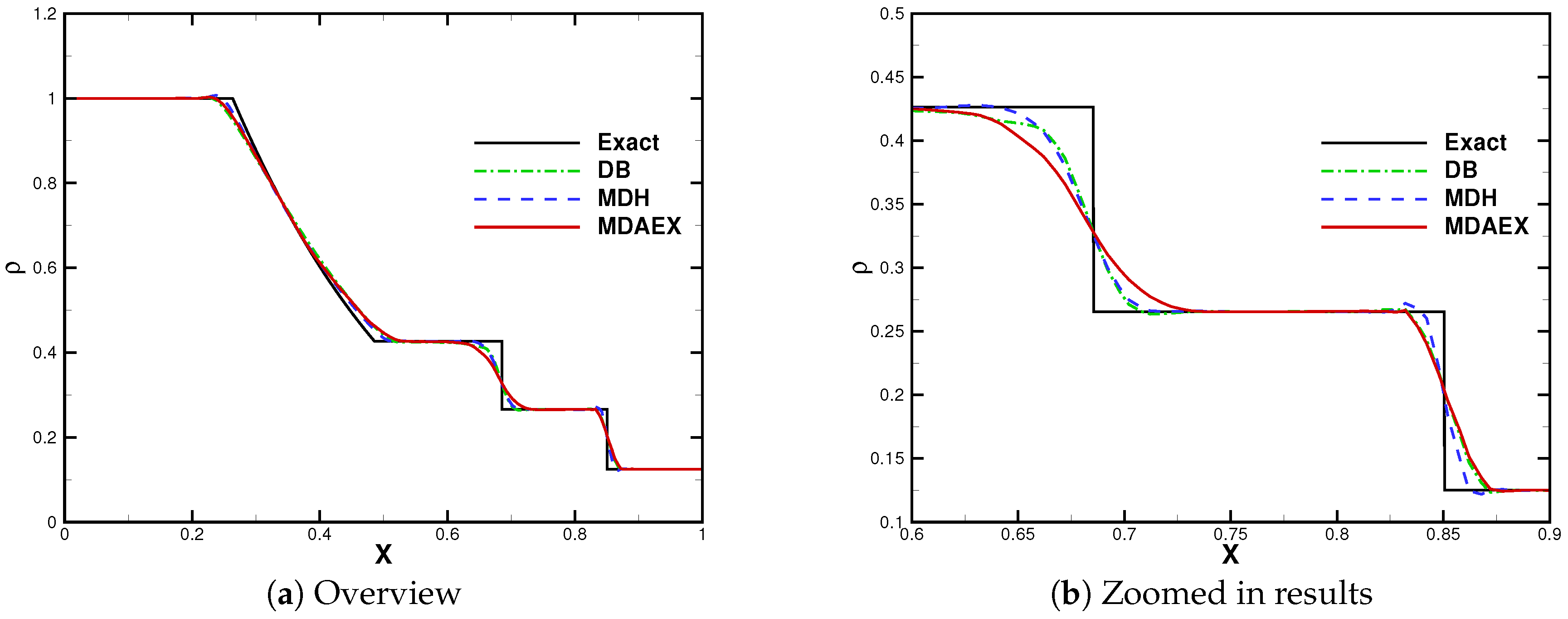
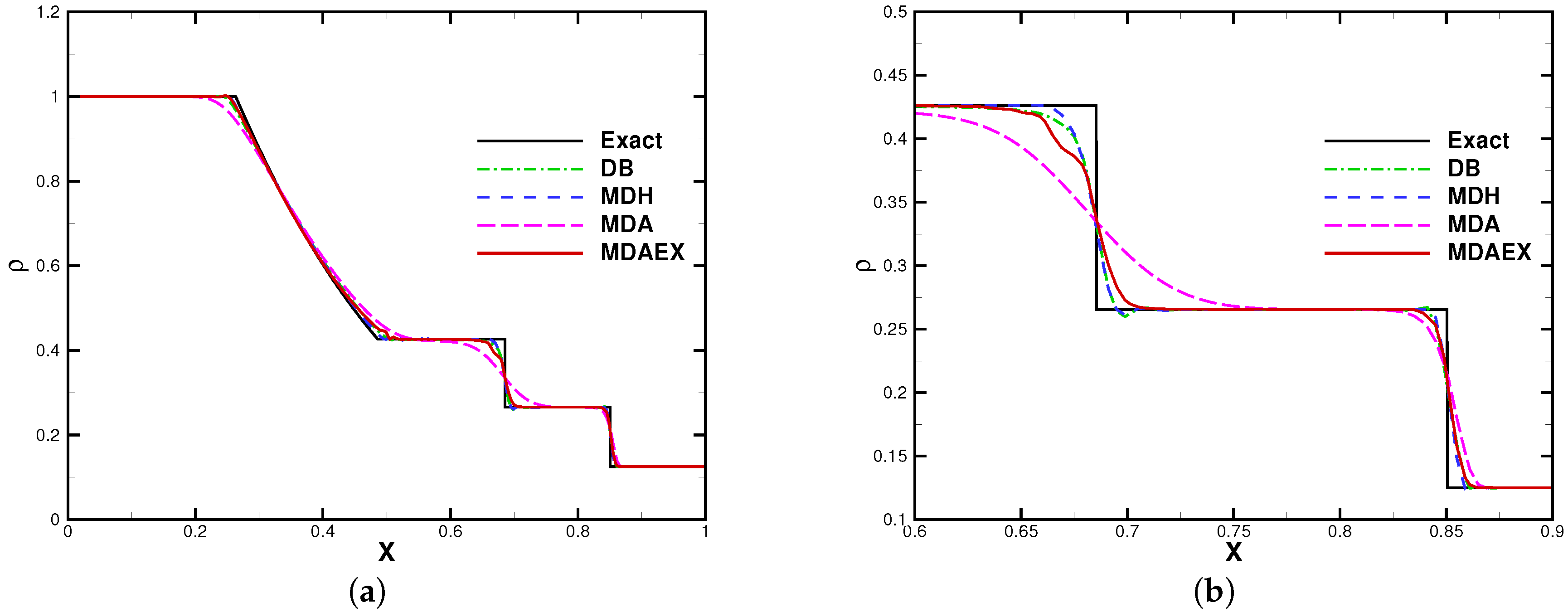
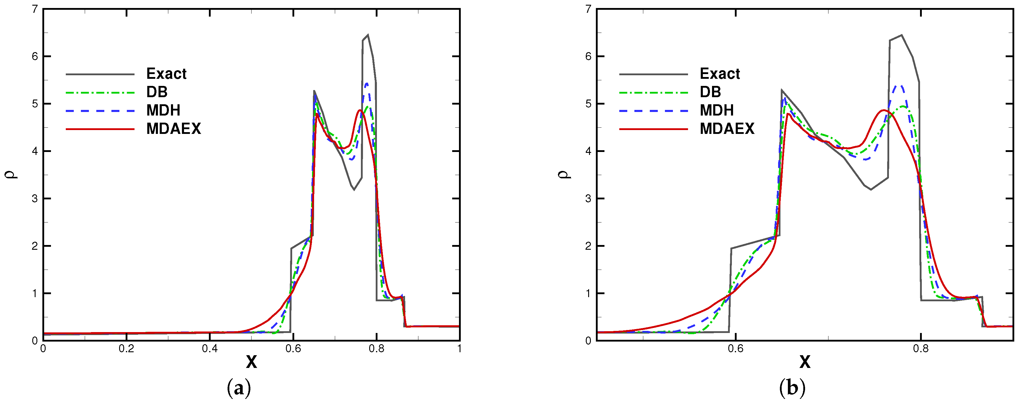
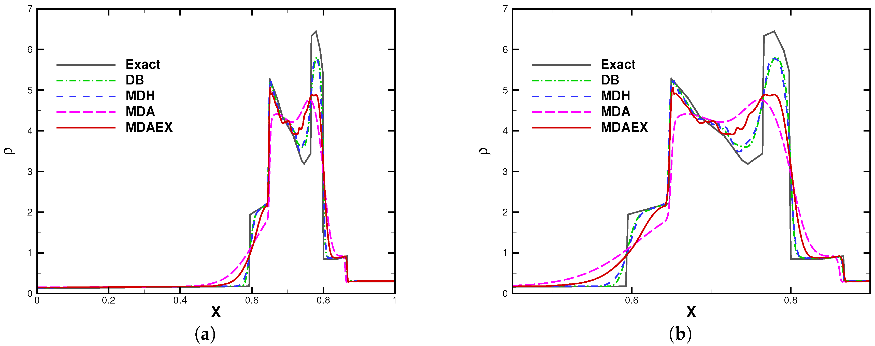
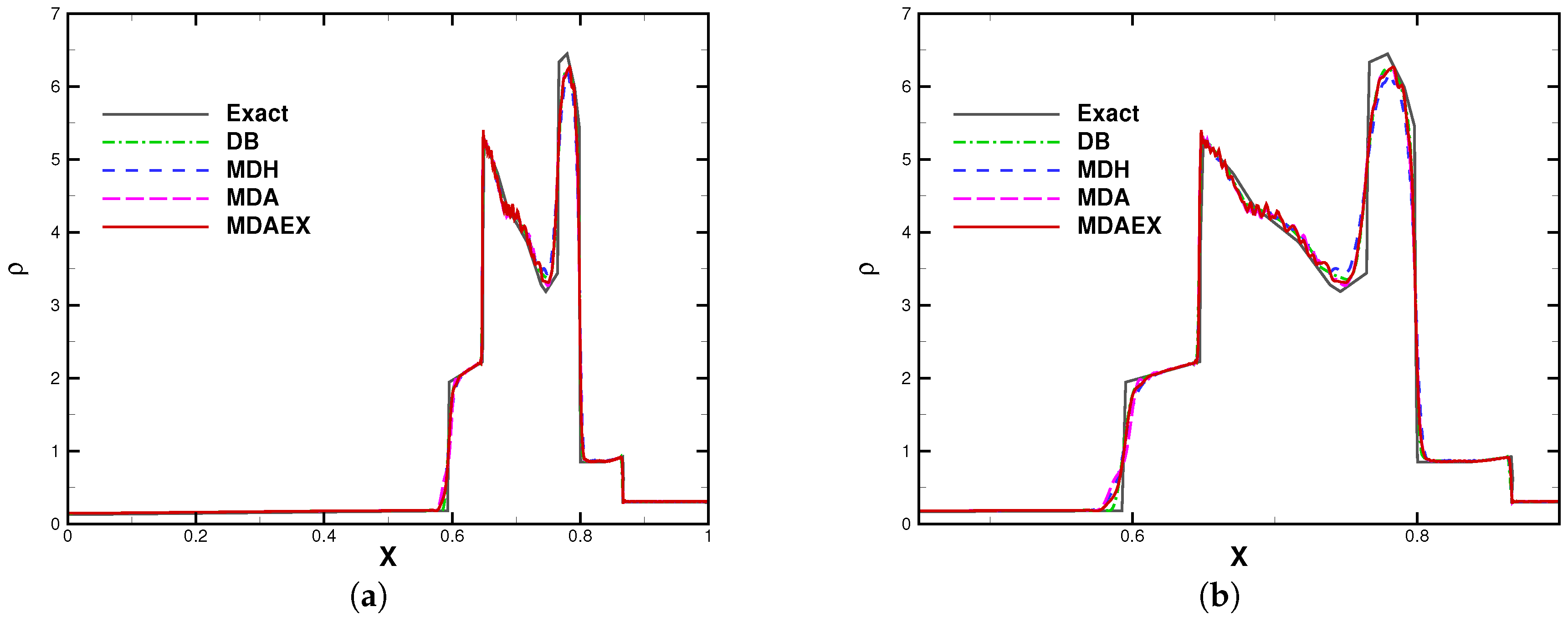
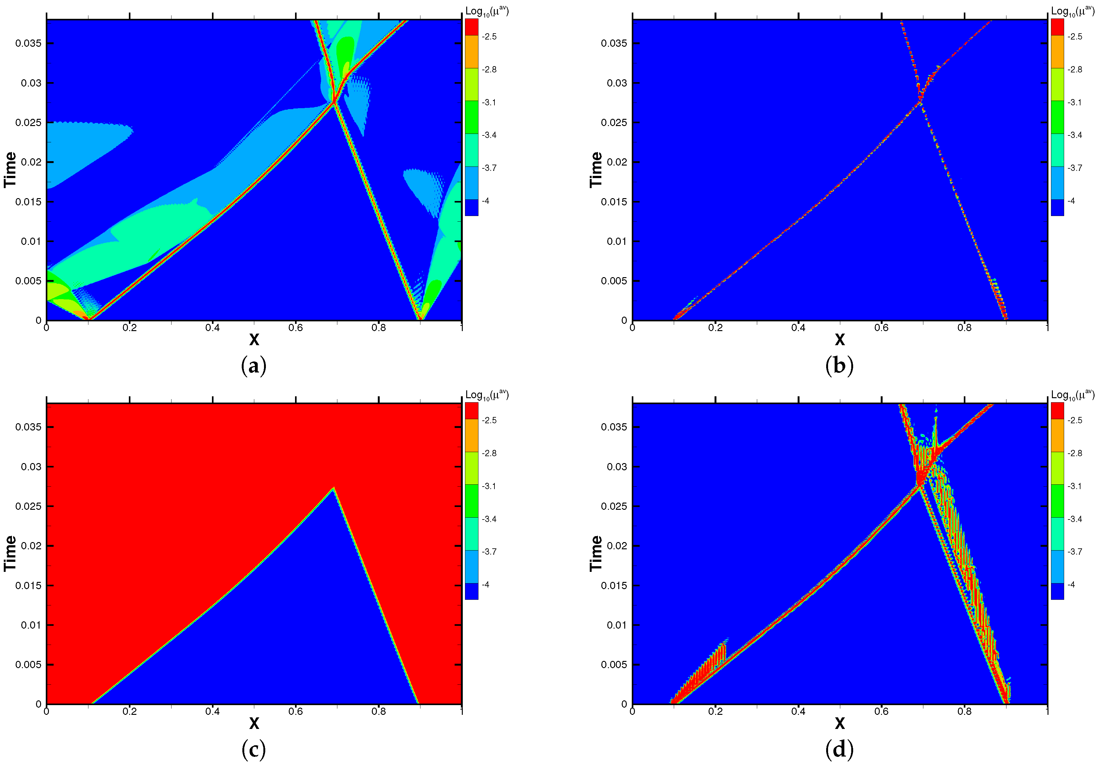
4.2.3. Blast Wave Problem

The blast wave problem involves very strong shocks, providing a good test case for shock-capturing approaches. The domain was chosen to be [ 0 , 1 ] with reflecting conditions applied on both boundaries. The initial condition is given as
( ρ , u , p ) = ( 1 , 0 , 1000 ) , x < 0.1 , ( 1 , 0 , 0.01 ) , 0.1 x 0.9 , ( 1 , 0 , 100 ) , x > 0.9 .
The number of elements was fixed to 300 for all of the computations. The solution is compared at t = 0.038 in Figure 13, Figure 14, Figure 15 and Figure 16. The reference solution was obtained with the fifth-order finite difference WENO scheme using 20,000 grid points. It can be observed that MDAEX is able to produce reasonable results from P 1 to P 4 . Furthermore, MDAEX is able to capture the complicated flow structures in a sharp manner, as shown in Figure 17.

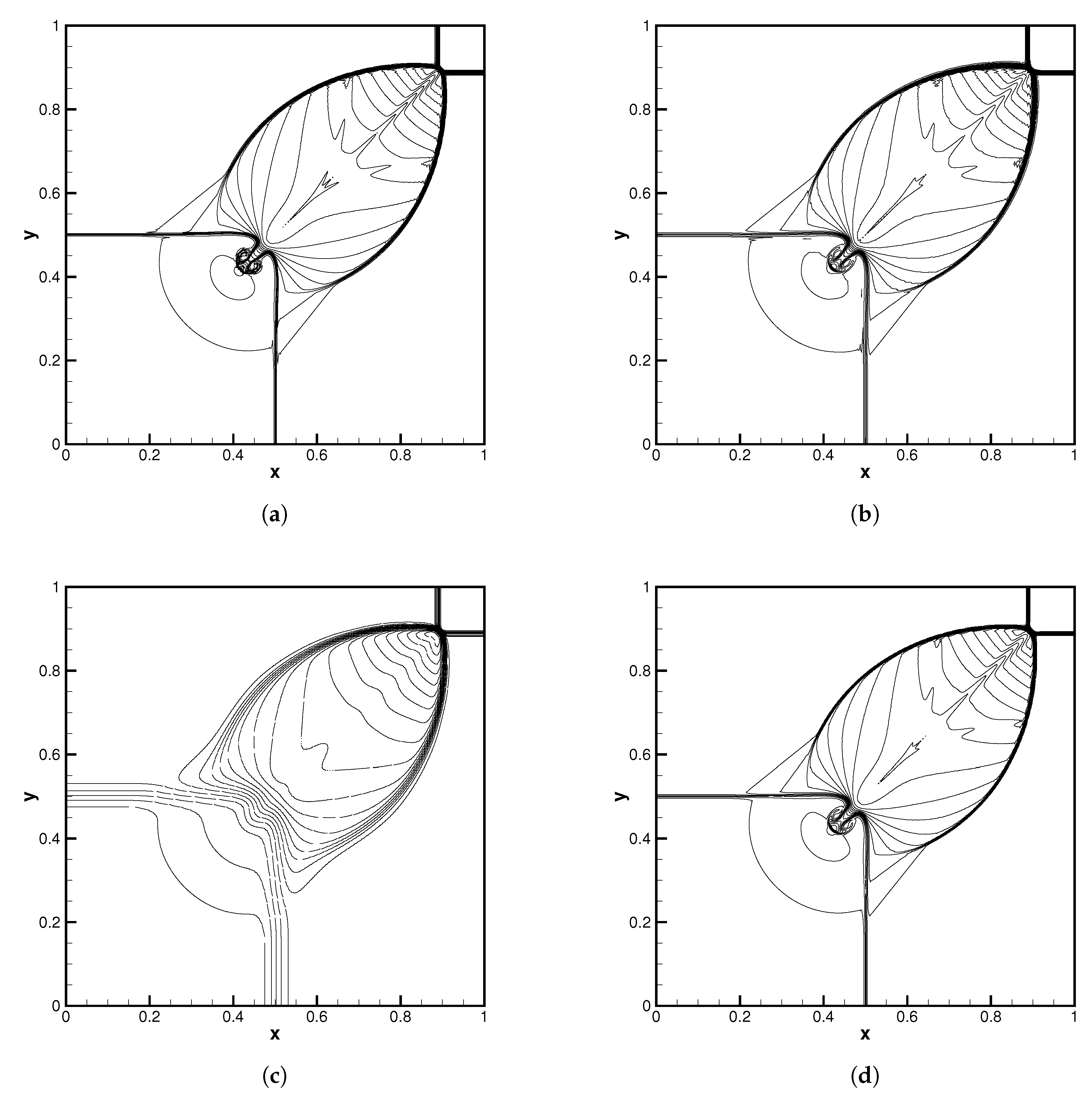
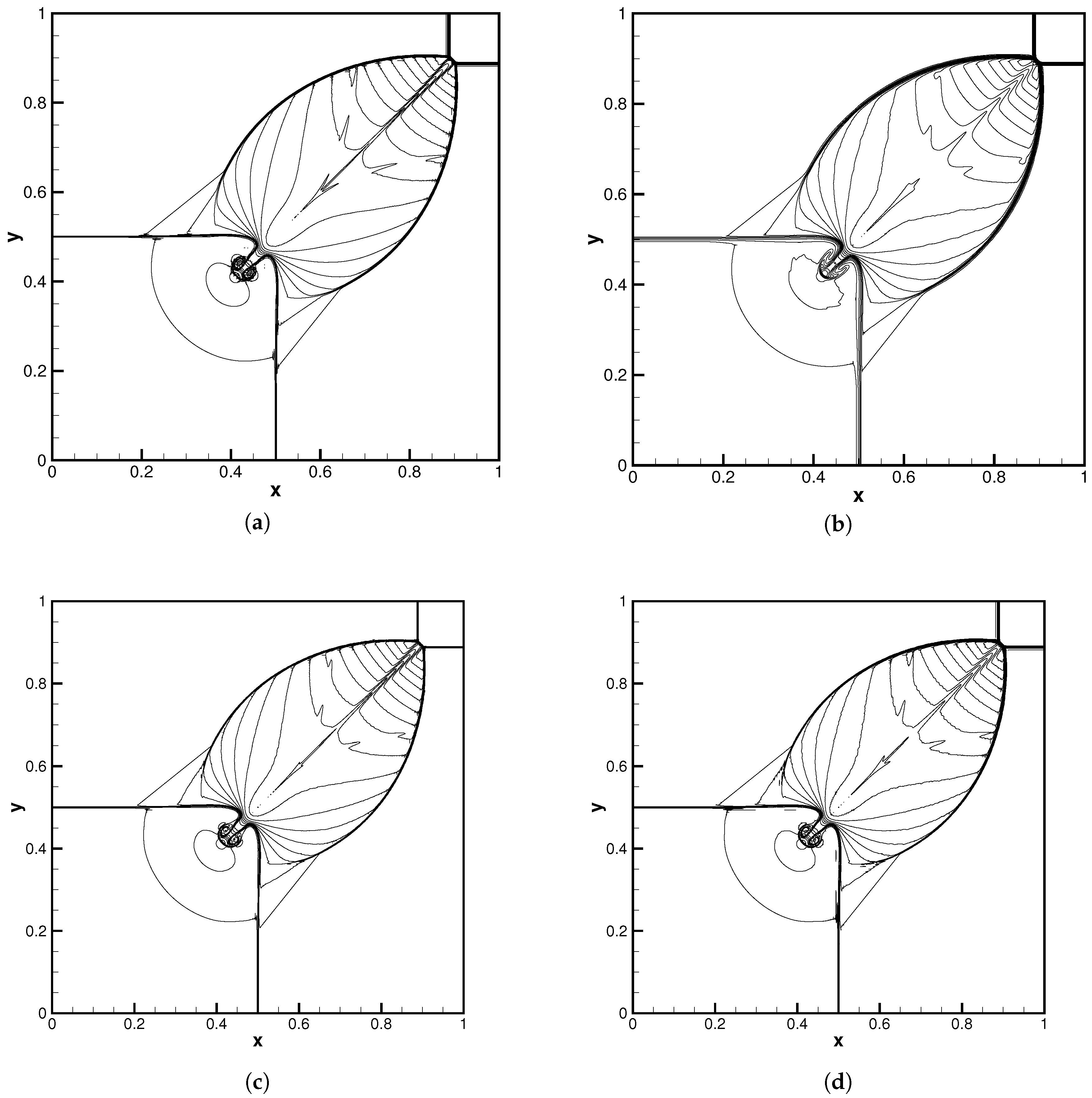
4.2.4. Two-Dimensional Riemann Problem

In this section, we considered a two-dimensional Riemann problem [36]. The computational domain is [ 0 , 1 ] × [ 0 , 1 ] , which is uniformly divided by quadrilateral elements. The number of elements along each edge was fixed to 160. For this case, the initial condition (known as Case 12) is given as
( ρ , u , v , p ) = ( 0.5313 , 0 , 0 , 0.4 ) , 0.5 < x < 1 , 0.5 < y < 1 , ( 1 , 0.7276 , 0 , 1 ) , 0 < x < 0.5 , 0.5 < y < 1 , ( 0.8 , 0 , 0 , 1 ) , 0 < x < 0.5 , 0 < y < 0.5 , ( 1 , 0 , 0.7276 , 1 ) , 0.5 < x < 1 , 0 < y < 0.5 .
The density contours at t = 0.25 are presented in Figure 18, Figure 19 and Figure 20. In P 2 , MDA behaves as overly dissipative, whereas MDAEX is able to produce a more reasonable result, which is similar to MDH but with less oscillation and dissipation. For P 3 , MDAEX is also among the least dissipative models. Note that all models produce reasonable results for P 4 .

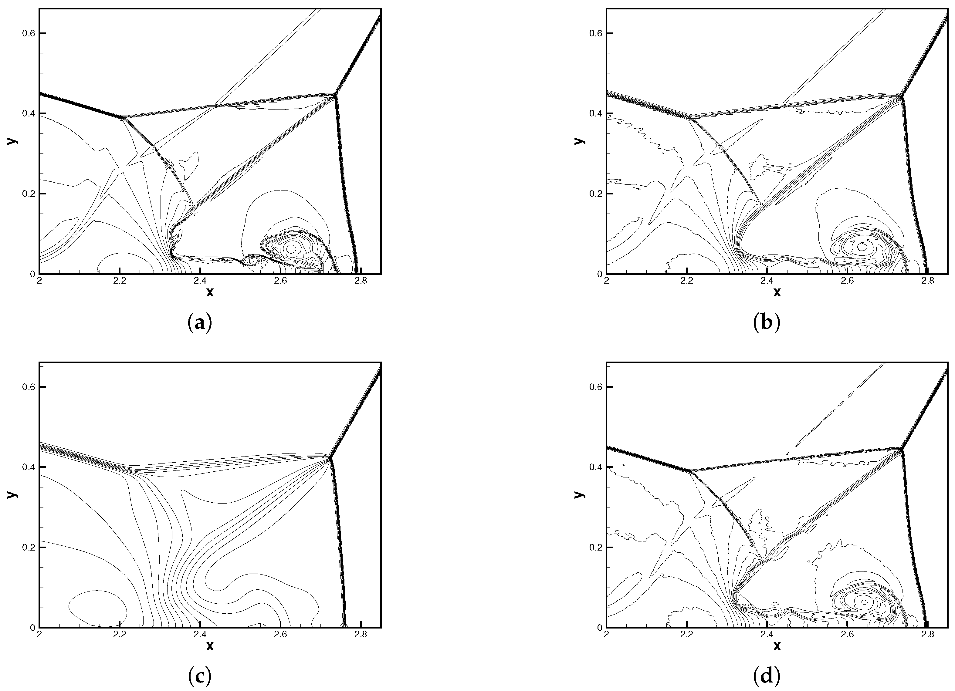
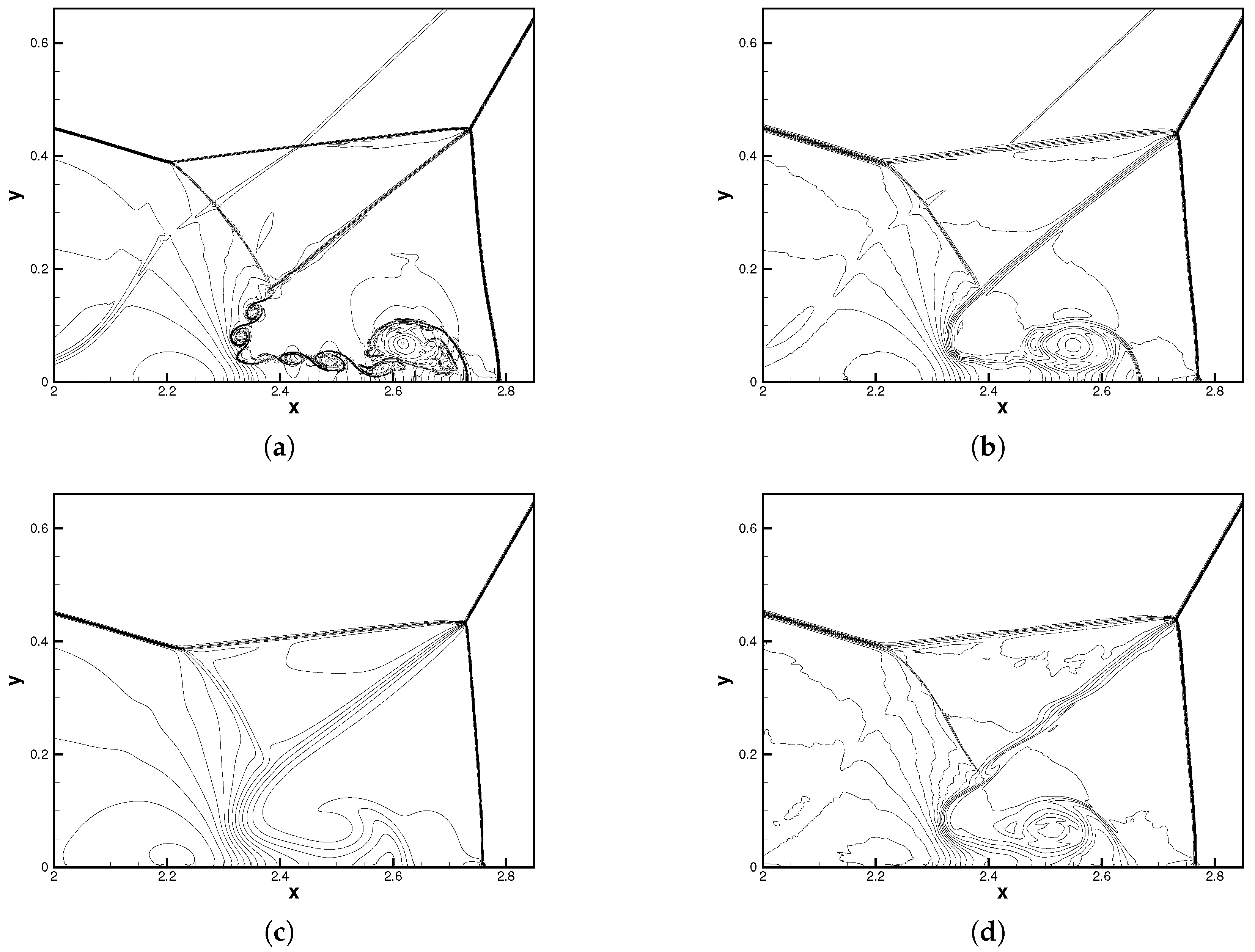
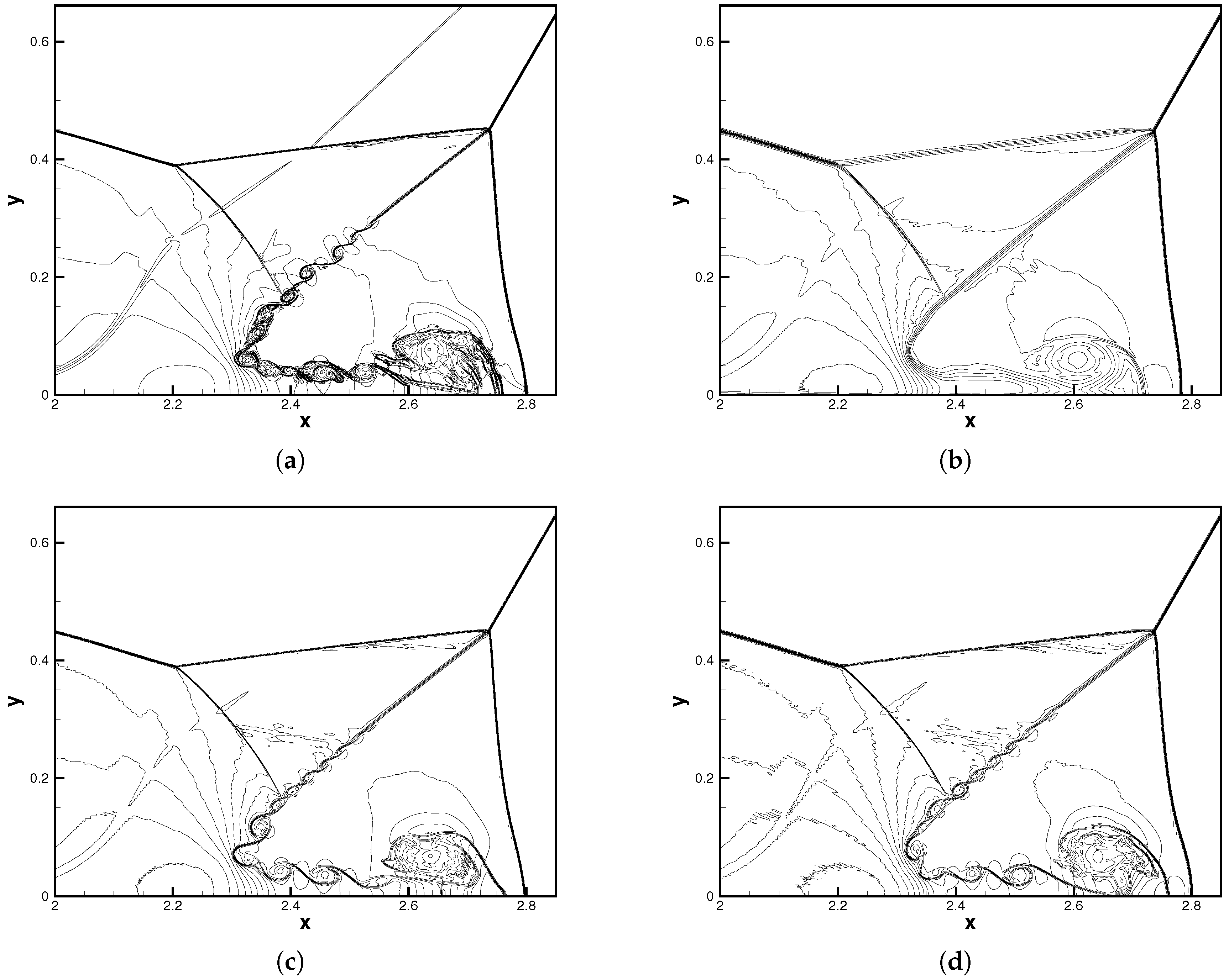
4.2.5. Double Mach Problem

The double Mach problem is a benchmark test case for shock-capturing methods. The computational domain is [ 0 , 4 ] × [ 0 , 1 ] . The left boundary was set to be the post condition of the shock, and the right boundary was extrapolation. The initial condition was formed by a Mach 10 shock making a 60 angle with the x-direction and intersecting with the x-axis at x = 1 / 6 . The upper boundary was prescribed to describe the motion of the Mach 10 shock. The inviscid wall condition spanned the region 1 / 6 < x < 4 of the bottom boundary, and the rest of it was set to the post-shock condition. The computation was conducted on a grid divided by 816 × 204 quadrilateral elements. Density contours at t = 0.2 are plotted in Figure 21, Figure 22 and Figure 23. It can be seen that DB is among the least dissipative models in this case. MDAEX is slightly less dissipative than MDH at P 2 and P 3 and similar to DB and MDA at P 4 . Note that the localized viscosity approach in Equation (23) significantly reduces numerical dissipation around the switch-off point of the viscosity model. Compared to the MDA model, the MDAEX model performs generally well among the three modal-decay-based models, especially at P 2 and P 3 .

5. Conclusions

In this paper, a modal-decay-based artificial viscosity model with a flux reconstruction method was proposed. The amount of added artificial viscosity was determined according to the decay rate of the expansion modes. Sufficient information is critical for an accurate estimation of the decay rate. Therefore, in order to ensure the performance of this type of model, especially for low orders ( P 2 and P 3 ), the information used to estimate the decay rate was augmented by combining the polynomials of the current element with its neighbors. Furthermore, in order to avoid excessive dissipation for the complex flow region, the scaling of the artificial viscosity was modified to ensure that the viscosity is of O ( h P + 1 ) close to the switch-off point of the model.
The proposed model (MDAEX) was applied to typical benchmark cases and compared with other typical models, including DB, MDH and MDA. Convergence tests with smooth flows show that MDAEX is able to recover the expected accuracy away from the coarsest grids for all of the polynomial orders considered in this paper. For shock-dominated flows, MDAEX was observed to capture delicate flow structures better for P 2 in terms of both the solutions and the distribution of artificial viscosity. For the proposed test cases, the MDAEX model serves as a more reasonable modal-decay-type model than the original MDA model in P 2 and P 3 -order. We note, however, that the behavior of the model for more complicated cases requires further investigation, which constitutes our future work.

Author Contributions

Conceptualization, C.Y. and J.Y.; formal analysis, L.M.; investigation, L.M. and J.Y.; resources, C.Y.; writing—original draft preparation, L.M. and J.Y.; writing—review and editing, L.M. and J.Y.; visualization, L.M.; supervision, C.Y. All authors have read and agreed to the published version of the manuscript.

Funding

This research was funded by the National Natural Science Foundation of China grant number No.11972064 and No.11721202.

Data Availability Statement

The data presented in this study are available on request from the corresponding author.

Conflicts of Interest

The authors declare no conflict of interest.

Abbreviations

The following abbreviations are used in this manuscript:
MDAaveraged modal decay
MDHhighest modal decay
MDAEXextended MDA
DBdilation-based
DGdiscontinuous Galerkin
SDspectral difference
FRflux reconstruction
CPRcorrection procedure via reconstruction
WENOweighted essentially non-oscillatory
HWENOHermite WENO
SPssolution points
SSPRK54strong stability preserving five-stage fourth-order Runge–Kutta

References

  1. Deng, X.; Mao, M.; Tu, G.; Liu, H.; Zhang, H. Geometric conservation law and applications to high-order finite difference schemes with stationary grids. J. Comput. Phys. 2011, 230, 1100–1115. [Google Scholar] [CrossRef]
  2. Friedrich, O. Weighted essentially non-oscillatory schemes for the interpolation of mean values on unstructured grids. J. Comput. Phys. 1998, 144, 194–212. [Google Scholar] [CrossRef]
  3. Cockburn, B.; Karniadakis, G.E.; Shu, C.W. Discontinuous Galerkin Methods: Theory, Computation and Applications; Springer Science & Business Media: Berlin/Heidelberg, Germany, 2012; Volume 11. [Google Scholar]
  4. Liu, Y.; Vinokur, M.; Wang, Z. Spectral difference method for unstructured grids I: Basic formulation. J. Comput. Phys. 2006, 216, 780–801. [Google Scholar] [CrossRef]
  5. Huynh, H.T. A flux reconstruction approach to high-order schemes including discontinuous Galerkin methods. In Proceedings of the 18th AIAA Computational Fluid Dynamics Conference, Miami, FL, USA, 25–28 June 2007; Volume 1, pp. 698–739. [Google Scholar] [CrossRef]
  6. Haga, T.; Gao, H.; Wang, Z.J. A High-Order Unifying Discontinuous Formulation for the Navier-Stokes Equations on 3D Mixed Grids. Math. Model. Nat. Phenom. 2011, 6, 28–56. [Google Scholar] [CrossRef] [Green Version]
  7. Hesthaven, J.S. Numerical Methods for Conservation Laws: From Analysis to Algorithms; SIAM: Philadelphia, PA, USA, 2017. [Google Scholar]
  8. Cockburn, B.; Shu, C.W. The Runge–Kutta discontinuous Galerkin method for conservation laws V: Multidimensional systems. J. Comput. Phys. 1998, 141, 199–224. [Google Scholar] [CrossRef]
  9. Burbeau, A.; Sagaut, P.; Bruneau, C.H. A problem-independent limiter for high-order Runge–Kutta discontinuous Galerkin methods. J. Comput. Phys. 2001, 169, 111–150. [Google Scholar] [CrossRef]
  10. Krivodonova, L. Limiters for high-order discontinuous Galerkin methods. J. Comput. Phys. 2007, 226, 879–896. [Google Scholar] [CrossRef]
  11. Qiu, J.; Shu, C.W. A comparison of troubled-cell indicators for Runge–Kutta discontinuous Galerkin methods using weighted essentially nonoscillatory limiters. SIAM J. Sci. Comput. 2005, 27, 995–1013. [Google Scholar] [CrossRef] [Green Version]
  12. Qiu, J.; Shu, C.W. Runge–Kutta discontinuous Galerkin method using WENO limiters. SIAM J. Sci. Comput. 2005, 26, 907–929. [Google Scholar] [CrossRef]
  13. Zhu, J.; Qiu, J.; Shu, C.W.; Dumbser, M. Runge–Kutta discontinuous Galerkin method using WENO limiters II: Unstructured meshes. J. Comput. Phys. 2008, 227, 4330–4353. [Google Scholar] [CrossRef]
  14. Qiu, J.; Shu, C.W. Hermite WENO schemes and their application as limiters for Runge–Kutta discontinuous Galerkin method: One-dimensional case. J. Comput. Phys. 2004, 193, 115–135. [Google Scholar] [CrossRef]
  15. Qiu, J.; Shu, C.W. Hermite WENO schemes and their application as limiters for Runge–Kutta discontinuous Galerkin method II: Two dimensional case. Comput. Fluids 2005, 34, 642–663. [Google Scholar] [CrossRef]
  16. Zhu, J.; Qiu, J. Hermite WENO schemes and their application as limiters for Runge-Kutta discontinuous Galerkin method, III: Unstructured meshes. J. Sci. Comput. 2009, 39, 293–321. [Google Scholar] [CrossRef]
  17. Zhong, X.; Shu, C.W. A simple weighted essentially nonoscillatory limiter for Runge–Kutta discontinuous Galerkin methods. J. Comput. Phys. 2013, 232, 397–415. [Google Scholar] [CrossRef]
  18. Zhu, J.; Zhong, X.; Shu, C.W.; Qiu, J. Runge–Kutta discontinuous Galerkin method using a new type of WENO limiters on unstructured meshes. J. Comput. Phys. 2013, 248, 200–220. [Google Scholar] [CrossRef]
  19. Cook, A.W.; Cabot, W.H. A high-wavenumber viscosity for high-resolution numerical methods. J. Comput. Phys. 2004, 195, 594–601. [Google Scholar] [CrossRef] [Green Version]
  20. Cook, A.W.; Cabot, W.H. Hyperviscosity for shock-turbulence interactions. J. Comput. Phys. 2005, 203, 379–385. [Google Scholar] [CrossRef]
  21. Fiorina, B.; Lele, S.K. An artificial nonlinear diffusivity method for supersonic reacting flows with shocks. J. Comput. Phys. 2007, 222, 246–264. [Google Scholar] [CrossRef] [Green Version]
  22. Kawai, S.; Lele, S.K. Localized artificial diffusivity scheme for discontinuity capturing on curvilinear meshes. J. Comput. Phys. 2008, 227, 9498–9526. [Google Scholar] [CrossRef]
  23. Mani, A.; Larsson, J.; Moin, P. Suitability of artificial bulk viscosity for large-eddy simulation of turbulent flows with shocks. J. Comput. Phys. 2009, 228, 7368–7374. [Google Scholar] [CrossRef]
  24. Premasuthan, S.; Liang, C.; Jameson, A. Computation of flows with shocks using the spectral difference method with artificial viscosity, I: Basic formulation and application. Comput. Fluids 2014, 98, 111–121. [Google Scholar] [CrossRef]
  25. Moro, D.; Nguyen, N.C.; Peraire, J. Dilation-based shock capturing for high-order methods. Int. J. Numer. Methods Fluids 2016, 82, 398–416. [Google Scholar] [CrossRef]
  26. Guermond, J.L.; Pasquetti, R.; Popov, B. Entropy viscosity method for nonlinear conservation laws. J. Comput. Phys. 2011, 230, 4248–4267. [Google Scholar] [CrossRef]
  27. Zingan, V.; Guermond, J.L.; Morel, J.; Popov, B. Implementation of the entropy viscosity method with the discontinuous Galerkin method. Comput. Methods Appl. Mech. Eng. 2013, 253, 479–490. [Google Scholar] [CrossRef]
  28. Chaudhuri, A.; Jacobs, G.B.; Don, W.S.; Abbassi, H.; Mashayek, F. Explicit discontinuous spectral element method with entropy generation based artificial viscosity for shocked viscous flows. J. Comput. Phys. 2017, 332, 99–117. [Google Scholar] [CrossRef] [Green Version]
  29. Persson, P.O.; Peraire, J. Sub-cell shock capturing for discontinuous Galerkin methods. In Proceedings of the 44th AIAA Aerospace Sciences Meeting and Exhibit, Reno, NV, USA, 9–12 January 2006; p. 112. [Google Scholar]
  30. Klöckner, A.; Warburton, T.; Hesthaven, J.S. Viscous shock capturing in a time-explicit discontinuous Galerkin method. Math. Model. Nat. Phenom. 2011, 6, 57–83. [Google Scholar] [CrossRef]
  31. Roe, P. Efficient construction and utilization of approximate Riemann solutions. Comput. Methods Appl. Sci. Eng. 1984, 6, 499–518. [Google Scholar]
  32. Peraire, J.; Persson, P.O. The compact discontinuous galerkin (CDG) method for elliptic problems. SIAM J. Sci. Comput. 2007, 30, 1806–1824. [Google Scholar] [CrossRef] [Green Version]
  33. Gottlieb, S. On high order strong stability preserving Runge-Kutta and multi step time discretizations. J. Sci. Comput. 2005, 25, 105–128. [Google Scholar] [CrossRef] [Green Version]
  34. Yu, J.; Hesthaven, J.S. A study of several artificial viscosity models within the discontinuous galerkin framework. Commun. Comput. Phys. 2020, 27, 1309–1343. [Google Scholar]
  35. Spiegel, S.C.; Huynh, H.; DeBonis, J.R. A survey of the isentropic Euler vortex problem using high-order methods. In Proceedings of the 22nd AIAA Computational Fluid Dynamics Conference, Dallas, TX, USA, 22–26 June 2015; p. 2444. [Google Scholar]
  36. Lax, P.D.; Liu, X.D. Solution of two-dimensional Riemann problems of gas dynamics by positive schemes. SIAM J. Sci. Comput. 1998, 19, 319–340. [Google Scholar] [CrossRef]
Figure 1. Illustration of the extended MDA sensor. The black dashed line is the original solution. The orange solid line is the modified solution in the current element e .
Aerospace 10 00014 g001
Figure 2. Illustration of quadrilateral elements for the two-dimensional shock-capturing model.
Aerospace 10 00014 g002
Figure 3. Density solution for the Sod problem with 100 elements at t = 0.2 , P 1 . (a) Overview; (b) zoomed in results.
Aerospace 10 00014 g003
Figure 4. Density solution for the Sod problem with 100 elements at t = 0.2 , P 2 . (a) Overview; (b) zoomed in results.
Aerospace 10 00014 g004
Figure 5. Density solution for the Sod problem with 100 elements at t = 0.2 , P 3 . (a) Overview; (b) zoomed in results.
Aerospace 10 00014 g005
Figure 6. Density solution for the Sod problem with 100 elements at t = 0.2 , P 4 . (a) Overview; (b) zoomed in results.
Aerospace 10 00014 g006
Figure 7. Temporal history of artificial viscosity for the one-dimensional Sod problem with 100 P 2 elements for t [ 0 , 0.2 ] . (a) DB; (b) MDH; (c) MDA; (d) MDAEX.
Aerospace 10 00014 g007
Figure 8. Density solution for the one-dimensional Shu–Osher problem with 200 elements at t = 1.8 , P 1 . (a) Overview; (b) zoomed in results.
Aerospace 10 00014 g008
Figure 9. Density solution for the one-dimensional Shu–Osher problem with 200 elements at t = 1.8 , P 2 . (a) Overview; (b) zoomed in results.
Aerospace 10 00014 g009
Figure 10. Density solution for the one-dimensional Shu–Osher problem with 200 elements at t = 1.8 , P 3 . (a) Overview; (b) zoomed in results.
Aerospace 10 00014 g010
Figure 11. Density solution for the one-dimensional Shu–Osher problem with 200 elements at t = 1.8 , P 4 . (a) Overview; (b) zoomed in results.
Aerospace 10 00014 g011
Figure 12. Temporal history of artificial viscosity for the one-dimensional Shu–Osher problem with 200 P2 elements for t [ 0 , 1.8 ] . (a) DB; (b) MDH; (c) MDA; (d) MDAEX.
Aerospace 10 00014 g012
Figure 13. Density solution for the blast wave problem with 300 elements at t = 0.038 , P 1 . (a) Overview; (b) zoomed in results.
Aerospace 10 00014 g013
Figure 14. Density solution for the blast wave problem with 300 elements at t = 0.038 , P 2 . (a) Overview; (b) zoomed in results.
Aerospace 10 00014 g014
Figure 15. Density solution for the blast wave problem with 300 elements at t = 0.038 , P 3 . (a) Overview; (b) zoomed in results.
Aerospace 10 00014 g015
Figure 16. Density solution for the blast wave problem with 300 elements at t = 0.038 , P 4 . (a) Overview; (b) zoomed in results.
Aerospace 10 00014 g016
Figure 17. Temporal history of artificial viscosity the blast wave problem with 300 P 2 elements for t [ 0 , 0.038 ] . (a) DB; (b) MDH; (c) MDA; (d) MDAEX.
Aerospace 10 00014 g017
Figure 18. Density solution for the two-dimensional Riemann problem (Case 12) with 160 × 160   P 2 elements at t = 0.25 . Thirty-one equally spaced contours from 0.515 to 1.665. (a) DB; (b) MDH; (c) MDA; (d) MDAEX.
Aerospace 10 00014 g018
Figure 19. Density solution for the two-dimensional Riemann problem (Case 12) with 160 × 160   P 3 elements at t = 0.25 . Thirty-one equally spaced contours from 0.515 to 1.665. (a) DB; (b) MDH; (c) MDA; (d) MDAEX.
Aerospace 10 00014 g019
Figure 20. Density solution for the two-dimensional Riemann problem (Case 12) with 160 × 160   P 4 elements at t = 0.25 . Thirty-one equally spaced contours from 0.515 to 1.665. (a) DB; (b) MDH; (c) MDA; (d) MDAEX.
Aerospace 10 00014 g020
Figure 21. Density solution for the double Mach problem with 816 × 204   P 2 elements at t = 0.2 . Thirty-three equally spaced contours from 1.75 to 22.7. (a) DB; (b) MDH; (c) MDA; (d) MDAEX.
Aerospace 10 00014 g021
Figure 22. Density solution for the double Mach problem with 816 × 204   P 3 elements at t = 0.2 . Thirty-three equally spaced contours from 1.75 to 22.7. (a) DB; (b) MDH; (c) MDA; (d) MDAEX.
Aerospace 10 00014 g022
Figure 23. Density solution for the double Mach problem with 816 × 204   P 4 elements at t = 0.2 . Thirty-three equally spaced contours from 1.75 to 22.7. (a) DB; (b) MDH; (c) MDA; (d) MDAEX.
Aerospace 10 00014 g023
Table 1. L 2 errors and accuracy orders of shock-capturing models for the one-dimensional linear transport.
NLinear DB MDH MDA MDAEX
L2 ErrorOrderL2 ErrorOrderL2 ErrorOrderL2 ErrorOrderL2 ErrorOrder
P 1 102.85 × 10 2 5.61 × 10 1 6.79 × 10 1 6.93 × 10 1
203.76 × 10 3 2.923.55 × 10 1 0.665.66 × 10 1 0.26 6.70 × 10 1 0.05
404.77 × 10 4 2.981.46 × 10 1 1.283.16 × 10 1 0.84 4.88 × 10 1 0.46
805.98 × 10 5 2.994.70 × 10 2 1.631.74 × 10 1 0.86 2.58 × 10 1 0.92
1607.49 × 10 6 3.001.31 × 10 2 1.848.79 × 10 2 0.99 7.49 × 10 6 15.07
3209.37 × 10 7 3.003.39 × 10 3 1.954.22 × 10 2 1.06 9.37 × 10 7 3.00
P 2 101.17 × 10 4 3.49 × 10 1 1.17 × 10 4 6.82 × 10 1 6.52 × 10 1
203.77 × 10 6 4.961.45 × 10 1 1.273.77 × 10 6 4.966.07 × 10 1 0.175.33 × 10 1 0.29
401.19 × 10 7 4.994.69 × 10 2 1.631.19 × 10 7 4.994.43 × 10 1 0.453.16 × 10 1 0.75
803.71 × 10 9 5.001.31 × 10 2 1.843.71 × 10 9 5.002.75 × 10 1 0.693.71 × 10 9 26.34
1601.16 × 10 10 5.003.39 × 10 3 1.951.16 × 10 10 5.001.55 × 10 1 0.831.16 × 10 10 5.00
3203.81 × 10 12 4.928.54 × 10 4 1.993.81 × 10 12 4.928.21 × 10 2 0.913.81 × 10 12 4.92
P 3 102.24 × 10 6 2.16 × 10 1 2.24 × 10 6 4.83 × 10 1 2.24 × 10 6
201.45 × 10 7 3.957.59 × 10 2 1.511.45 × 10 7 3.953.23 × 10 1 0.581.45 × 10 7 3.95
409.11 × 10 9 3.992.25 × 10 2 1.759.11 × 10 9 3.991.91 × 10 1 0.769.11 × 10 9 3.99
805.70 × 10 10 4.005.96 × 10 3 1.925.70 × 10 10 4.001.05 × 10 1 0.875.70 × 10 10 4.00
1603.59 × 10 11 3.991.51 × 10 3 1.983.59 × 10 11 3.995.48 × 10 2 0.933.59 × 10 11 3.99
3202.69 × 10 12 3.743.80 × 10 4 1.992.69 × 10 12 3.742.81 × 10 2 0.972.69 × 10 12 3.74
P 4 104.54 × 10 7 1.43 × 10 1 4.54 × 10 7 4.54 × 10 7 4.54 × 10 7
201.45 × 10 8 4.974.64 × 10 2 1.621.45 × 10 8 4.971.45 × 10 8 4.971.45 × 10 8 4.97
404.56 × 10 10 4.991.31 × 10 2 1.834.56 × 10 10 4.994.56 × 10 10 4.994.56 × 10 10 4.99
801.48 × 10 11 4.953.38 × 10 3 1.951.48 × 10 11 4.951.48 × 10 11 4.951.48 × 10 11 4.95
1605.76 × 10 13 4.688.54 × 10 4 1.995.76 × 10 13 4.685.75 × 10 13 4.685.75 × 10 13 4.68
Table 2. L 2 errors and accuracy orders of shock-capturing models for the two-dimensional isentropic vortex convection.
NLinear DB MDH MDA MDAEX
L2 ErrorOrderL2 ErrorOrderL2 ErrorOrderL2 ErrorOrderL2 ErrorOrder
P 1 404.10 × 10 3 1.70 × 10 2 1.52 × 10 2 3.25 × 10 2
805.51 × 10 4 2.905.18 × 10 3 1.715.28 × 10 3 1.53 2.81 × 10 2 0.21
1606.41 × 10 5 3.107.98 × 10 4 2.706.41 × 10 5 6.36 1.83 × 10 2 0.62
3208.95 × 10 6 2.841.02 × 10 4 2.968.95 × 10 6 2.84 5.65 × 10 3 1.69
6401.59 × 10 6 2.491.29 × 10 5 2.991.59 × 10 6 2.49 4.48 × 10 4 3.65
P 2 202.45 × 10 3 1.03 × 10 2 1.83 × 10 2 3.27 × 10 2 3.30 × 10 2
402.24 × 10 4 3.451.68 × 10 3 2.624.99 × 10 3 1.883.18 × 10 2 0.042.86 × 10 2 0.21
803.18 × 10 5 2.811.88 × 10 4 3.163.18 × 10 5 7.292.96 × 10 2 0.101.41 × 10 2 1.02
1605.97 × 10 6 2.421.90 × 10 5 3.315.97 × 10 6 2.422.54 × 10 2 0.221.59 × 10 3 3.15
3201.10 × 10 6 2.431.86 × 10 6 3.351.10 × 10 6 2.431.92 × 10 2 0.401.10 × 10 6 10.49
P 3 207.31 × 10 4 3.57 × 10 3 1.92 × 10 2 3.07 × 10 2 3.24 × 10 2
403.24 × 10 5 4.501.35 × 10 4 4.723.24 × 10 5 9.212.74 × 10 2 0.161.93 × 10 2 0.75
806.70 × 10 7 5.602.65 × 10 6 5.686.70 × 10 7 5.602.20 × 10 2 0.326.70 × 10 7 14.81
1601.32 × 10 8 5.667.25 × 10 8 5.191.32 × 10 8 5.661.52 × 10 2 0.541.32 × 10 8 5.66
3204.99 × 10 10 4.732.18 × 10 9 5.064.99 × 10 10 4.739.13 × 10 3 0.734.99 × 10 10 4.73
P 4 201.16 × 10 4 5.51 × 10 4 1.80 × 10 2 4.69 × 10 4 8.93 × 10 3
401.04 × 10 6 6.806.89 × 10 6 6.321.04 × 10 6 14.071.04 × 10 6 8.811.04 × 10 6 13.06
806.10 × 10 8 4.102.11 × 10 7 5.036.10 × 10 8 4.106.10 × 10 8 4.106.10 × 10 8 4.10
1602.87 × 10 9 4.417.57 × 10 9 4.802.87 × 10 9 4.412.87 × 10 9 4.412.87 × 10 9 4.41
3201.89 × 10 10 3.932.89 × 10 10 4.711.89 × 10 10 3.931.89 × 10 10 3.931.89 × 10 10 3.93
Disclaimer/Publisher’s Note: The statements, opinions and data contained in all publications are solely those of the individual author(s) and contributor(s) and not of MDPI and/or the editor(s). MDPI and/or the editor(s) disclaim responsibility for any injury to people or property resulting from any ideas, methods, instructions or products referred to in the content.

