Grassland Growth in Response to Climate Variability in the Upper Indus Basin, Pakistan

Abstract

Grasslands in the upper Indus basin provide a resource base for nomadic livestock grazing which is one of the major traditional livelihood practices in the area. The study presents climate patterns, grassland phenology, productivity and spatio-temporal climate controls on grassland growth using satellite data over the upper Indus basin of the Himalayan region, Pakistan. Phenology and productivity metrics of the grasses were estimated using a combination of derivative and threshold methods applied on fitted seasonal vegetation indices data over the period of 2001–2011. Satellite based rainfall and land surface temperature data are considered as representative explanatory variables to climate variability. The results showed distinct phenology and productivity patterns across four bioclimatic regions: (i) humid subtropical region (HSR)—late start and early end of season with short length of season and low productivity (ii) temperate region (TR)—early start and late end of season with higher length of season and moderate productivity (iii) sub alpine region (SAR)—late start and late end of season with very high length of season and the most productive grasses, and (iv) alpine region (AR)—late start and early end of season with small length of season and least productive grasses. Grassland productivity is constrained by temperature in the alpine region and by rainfall in the humid sub-tropical region. Spring temperature, winter and summer rainfall has shown significant and varied impact on phenology across different altitudes. The productivity is being influenced by summer and annual rainfall in humid subtropical regions, spring temperature in alpine and sub-alpine regions and both temperature and rainfall are contributing in temperate regions. The results revealing a strong relationship between grassland dynamics and climate variability put forth strong signals for drawing more scientific management of rangelands in the area.

1. Introduction

Grasslands occupy around half of the Hindu Kush Himalayan region, which provides a resource base for nomadic livestock grazing as well as associated ecosystem services such as maintaining biodiversity and avoiding the erosion that might result from cropping systems. The quality of grasslands is declining, primarily due to human-induced modifications such as agriculture, extensive livestock grazing, and invasive species, and they are further threatened by the potential effects of a changing climate. The high altitude grasslands in mountainous areas including the Himalayas are thought to be especially critical in terms of susceptibility to climate change [1,2]. The upper Indus basin (UIB) is a particularly complex area of the Hindu Kush Himalayas because of the high climatic variability on a relatively small scale [3]. The pastoralists must adapt to the changes in climatic conditions to ensure sustainable grazing plans, but they need support including providing information on vegetation and climate patterns in the area. Unless the local dynamics of the grassland ecosystem are understood and used as guidelines for development policies, interventions are likely to be random activities that comprise development by trial and error [4]. There are few studies on rangeland conditions and their relationship with climate factors and change in the Himalayas and the studies that have been done were mostly qualitative and based on focus group discussions and interviews [5]. A systematic assessment is needed to understand the grasslands dynamics in the region as a basis for devising appropriate policies for management.

Globally, a significant amount of work has been done on the use of satellite-based products for assessment of vegetation conditions and their related dynamics. Considering its vastness and the inaccessibility of the Hindu Kush Himalayan region, satellite-based measurements offer the only viable methodology for making assessments over anything but very small areas. With reference to vegetation assessment studies, NDVI (normalized difference vegetation index) derived from remote sensing instruments is used as a proxy to measure vegetation biomass and associated dynamics [6,7] Annual production and net carbon dioxide flux are generally assumed to relate directly to NDVI integrated over the growing season [8] and NDVI has shown consistent correlation with vegetation biomass and dynamics in various ecosystems worldwide (e.g., [9,10,11,12,13,14,15,16] Several studies have used remote sensing along with process models to analyze patterns and timing of anomalies in net primary productivity [17,18].

In the nomadic livestock grazing (transhumance) system, the migration cycle is primarily dictated by the local climatic conditions and seasonal forage availability. Phenological parameters such as onset of greenness and length of growing season can be affected by short-term climate fluctuations such as temperature and rainfall, as well as anthropogenic activities, such as groundwater extraction and urbanization. In the longer term, annual phenology may change as a result of climate change and large scale anthropogenic disturbance [18,19,20]. Thus, differentiation of annual, inter-annual, and long-term phenological patterns is an important component in monitoring and modelling of global ecosystems [21] and may lead to better understanding of how vegetation cover changes over time [16].

In this context, our research aims to provide an understanding on ongoing climatic conditions and their impact on the grassland growth dynamics in the UIB. The specific questions addressed are: (1) what are the significant spatial patterns and temporal variability of grassland phenological calendars and productivity across the basin? (2) how are the spatial and temporal patterns of grassland calendars and production controlled as a function of climate?

2. Materials and Methods

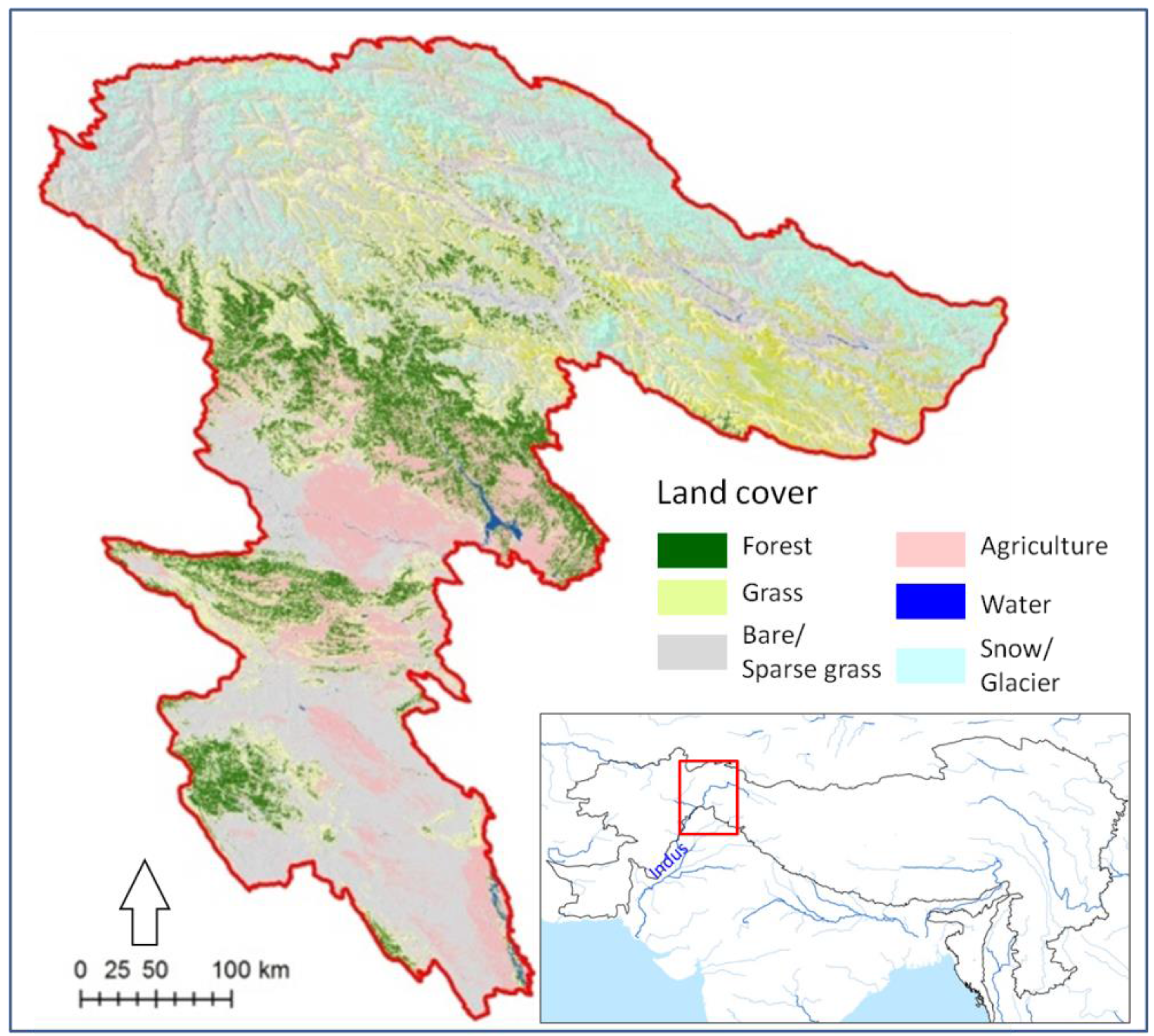
2.1. Study Area

Geographically, the study area lies between 31°N to 37°N and 69°E to 78°E with a total area of ~17 million∙ha, and is comprised of two provinces of Pakistan: Khyber Pakhtunkhwa (KP) and Gilgit-Balitistan (GB) (Figure 1). The area has diverse topography with alluvial plains, low hills, and high mountains of HKH. The vertical profile of the area ranges from 125 m in the south to about 8000 m in the north. The northern part of the UIB has a typically continental steppe climate, and precipitation is concentrated in winter and spring [22]. At high elevations in the Hindu Kush, snowfall is much heavier and consequently large glaciers are a prominent feature of the landscape. Temperature in the valley areas varies between 30 °C in July to as low as 0 °C in January. In south, the climate becomes more typical of the Indian subcontinent, although a considerable proportion of the annual precipitation still comes from frontal cloud zones during the winter months. The combination of a short but powerful summer monsoon with frequent winter cloud zones gives a bimodal rainfall regime. In accordance with ecological regions in Pakistan [23], major grassland regimes in the study area are characterized with four bioclimatic regions (Table S1).

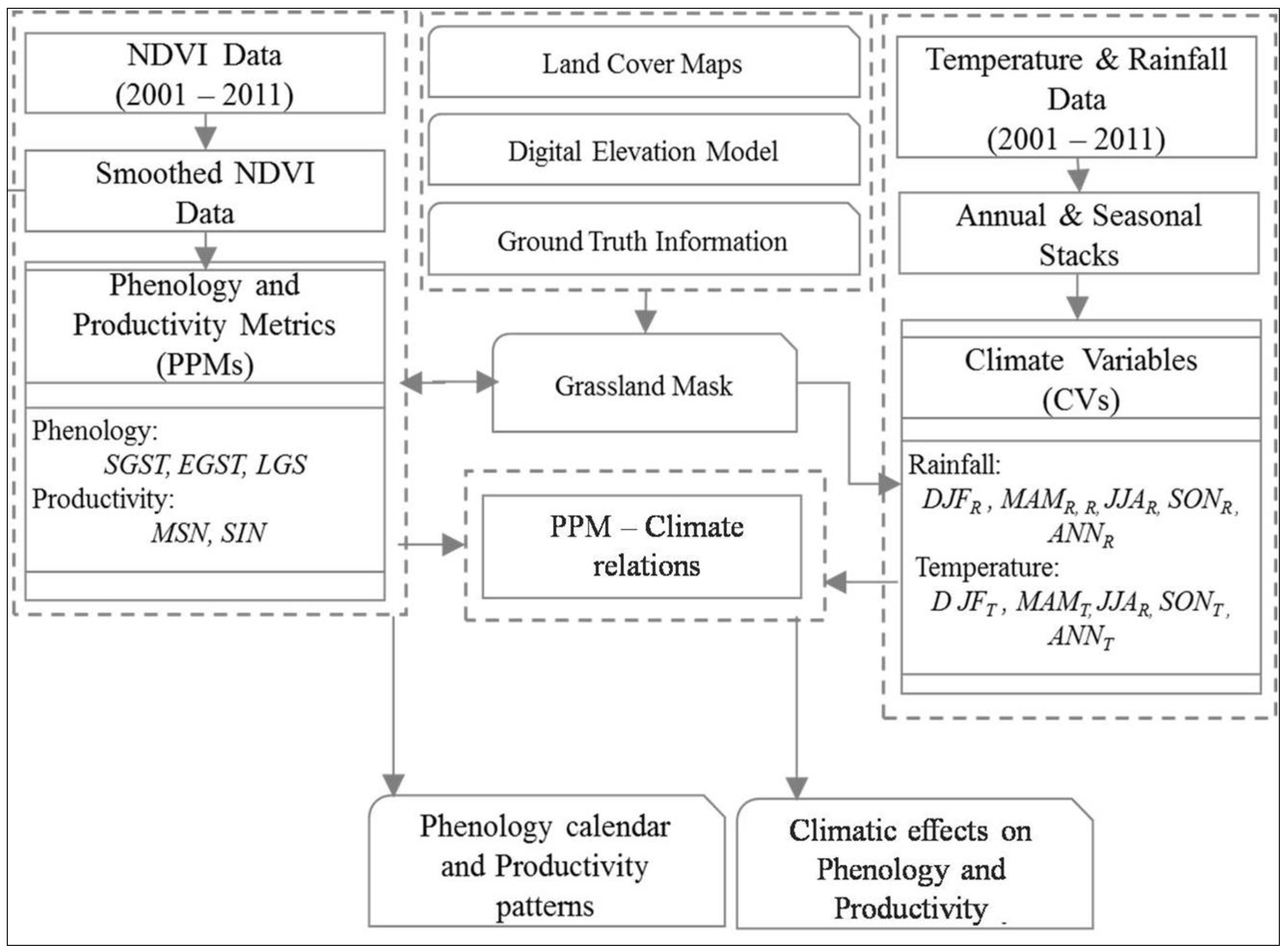
2.2. Methods Summary

A brief flow chart of methods are illustrated in Figure 2 (for details please see supplementary material). Normalised Difference Vegetation Index (NDVI) data, from moderate resolution sensor (MODIS) images taken at 16-day intervals and 250 m spatial resolution provided in a standard product (MOD13Q1, Level 3 Product), were used to extract phenology and productivity metrics (PPMs) of the grasslands: start of growing season (SGS), end of growing season (EGS) and length of growing season (LGS), seasonally integrated NDVI (SIN), and maximum seasonal NDVI (MSN) [24] (Table S2). The selected metrics were chosen to reveal spatio-temporal response patterns of grasslands to climatic variables [11,25,26,27,28]. Grassland was masked to avoid the contribution of numerous vegetation types present in the area. In the region, altitude is considered as a proxy to micro-climatic zones—therefore, altitudinal gradient was stratified into 10 classes of 500 m elevation intervals (ranges from <500 m to >4500 m) to minimize the effect of spatial variance. Land Surface Temperature (LST), from the MODIS MOD11C3 product, which provides monthly estimates of LST with a spatial resolution of 0.05° × 0.05° (~5.6 km at the equator), and Tropical Rainfall Measurement Mission (TRMM) data (3B43 product) were used to derive ten the climate variables (CVs)—seasonal and annual temperature, and rainfall. The PPMs and CVs were aggregated to give a spatial average per elevation zone [24,29]. The year-to-year response of PPMs to CVs was evaluated through the regression models [29]. For summarizing the results and discussion, the elevation zones were broadly categorized into four bioclimatic regions—that are: Humid subtropical region (HSR), Temperate region (TR), Subalpine region (SAR), Alpine region (AR).

Figure 1. Map of the Upper Indus basin (study area) showing land cover and location within the Hindu Kush Himalayan region.

Figure 1. Map of the Upper Indus basin (study area) showing land cover and location within the Hindu Kush Himalayan region.

Figure 2. Summary of methodology (see Supplementary 1 for detailed methods).

Figure 2. Summary of methodology (see Supplementary 1 for detailed methods).

3. Results

3.1. Relationship between Phenology Metrics and Temperature

Predominantly, the topography of the area is characterized with latitudinal and elevation gradient. The rainfall and temperature had large variability among season and across the elevation gradient. Valleys in mountainous areas were warmer ranging between 15 °C to 30 °C as compared to 0 °C to −15 °C on the mountains. Rainfall was relatively low in all elevation zones in autumn; in the humid subtropical region, it was highest in summer, whereas in the upper part of the temperate region it was lower in summer than in winter or spring; and in the sub alpine and alpine regions, it was highest in spring. Generally, temperature exhibited high spatial variability and low temporal variability while rainfall exhibited low spatial variability and high temporal variability (Table 1 and Table 2, Figure 3). The Humid Sub tropical zone was found with high rainfall and high temperature and high rainfall variability consisting of three seasons. On a relative scale, the temperate zone has medium rainfall and temperature with less variability of rainfall and temperature between peak and lean seasons. The alpine zone was found contrastingly with high rainfall and low temperature but with high degree of variation in Min–Max rainfall and temperature. This characteristic climatic variability delineated using satellite data across the elevation regimes broadly agrees with reported bioclimatic thresholds [23].

Figure 3. Distribution of bioclimatic zones against seasonal temperature and precipitation conditions in the study area.

Figure 3. Distribution of bioclimatic zones against seasonal temperature and precipitation conditions in the study area.

Functional relationship between NDVI-based phenology and productivity metrics and the ten climate variables has been examined to elaborate inter-annual variation in vegetation dynamics across the ten elevation zones. In understanding physical meanings of these linear correlations, it is important to consider consequent classes, coefficient of correlation (R), and the corresponding CVs. In addition, plant responses to climate variables may also be specific. Statistically significant correlations (p < 0.05) derived from linear regression analyses of phenology and productivity metrics with climate variables are shown in (Tables S3–S7).

The start of growing season showed a significant positive correlation with spring temperature in the humid subtropical region and winter temperature in the temperate region, and a negative correlation with spring temperature in the sub alpine and alpine regions (Table S3). The end of growing season only showed one significant correlation—with summer temperature in the lower zone of the humid subtropical region (Table S4). The lack of significant relationships especially over EGS could be due to the seasonal averages used for the relationship. We expect that the seasonal minimas of temperature and rainfall, which explain temperature and moisture stress, could have resulted in better explanation of EGS. The length of growing season showed a significant negative correlation with summer temperature in the humid subtropical region, winter temperature in the temperate region—while a positive correlation is observed with annual temperature in the humid subtropical region, temperate region, subalpine, and alpine regions and also with spring temperature in the subalpine and alpine regions. (Table S5).

The maximum seasonal NDVI showed a significant negative correlation with spring and summer temperature in the temperate region and annual temperature in the humid subtropical region and temperate regions (Table S6). The seasonally integrated NDVI showed a significant negative correlation with winter, spring, summer, and annual temperatures in the temperate zone, and a significant positive correlation with spring and annual temperature in the subalpine and alpine regions, and summer temperature in the higher alpine zone (Table S7).

3.2. Relationship between Phenology Metrics and Rainfall

There was only a small amount of correlation between growing season and rainfall. The start of growing season showed a significant positive correlation with winter rainfall and negative correlation with spring rainfall in the humid subtropical while in the subalpine region a positive correlation with winter rainfall (Table S7). The end of growing season only showed significant positive correlation with summer rainfall in the subalpine region (Table S4). The length of growing season showed significant positive correlation with summer rainfall in the subalpine region and negative correlation with winter rainfall in the alpine region (Table S5).

The maximum seasonal NDVI showed a significant positive correlation with winter rainfall in the lower part of the temperate region, with spring rainfall in the temperate region and upper part of the humid subtropical region, and with summer and annual rainfall humid subtropical region. (Table S6). The seasonally integrated NDVI showed a similar pattern to the maximum seasonal NDVI with the addition of a significant positive correlation with summer rainfall in the subalpine region (Table S7.). There was no significant correlation between productivity variables and rainfall in the alpine region.

Collectively, it can be deduced from above results, that seasonal productivity of the most productive grassland communities, zone 7 and zone 8, was influenced by EGS dependent upon JJA_R, due to which lengthening or shortening of LGS tended to increase or decrease in Seasonal Integrated NDVI.. Similarly, the negative relation of SIN and LGS with DJF_R in high alpine zones (Zone 9 and Zone 10) was unexplained as both EGS and SGS, and MSN do not portray any relation with DJF_R. It was interesting to note that the seasonal productivity (SIN) of low (<1000 m) and mid-altitude (1000 m to 3000 m) grassland communities is more dependent upon increase in MSN due to rainfall event rather the variation in LGS.

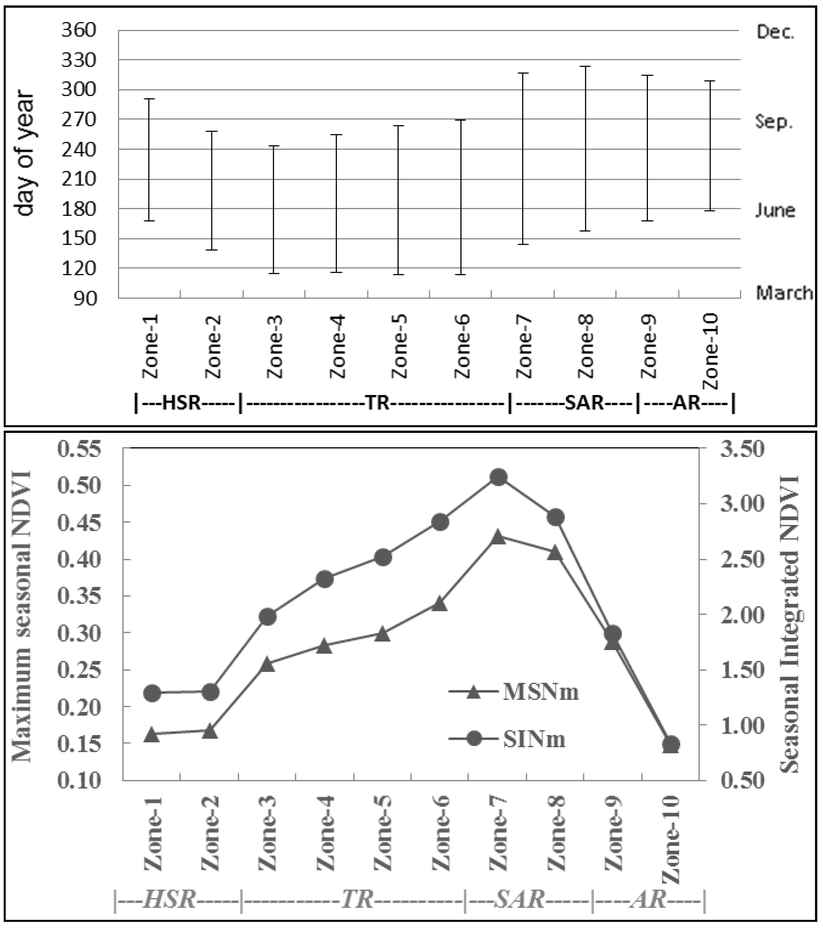
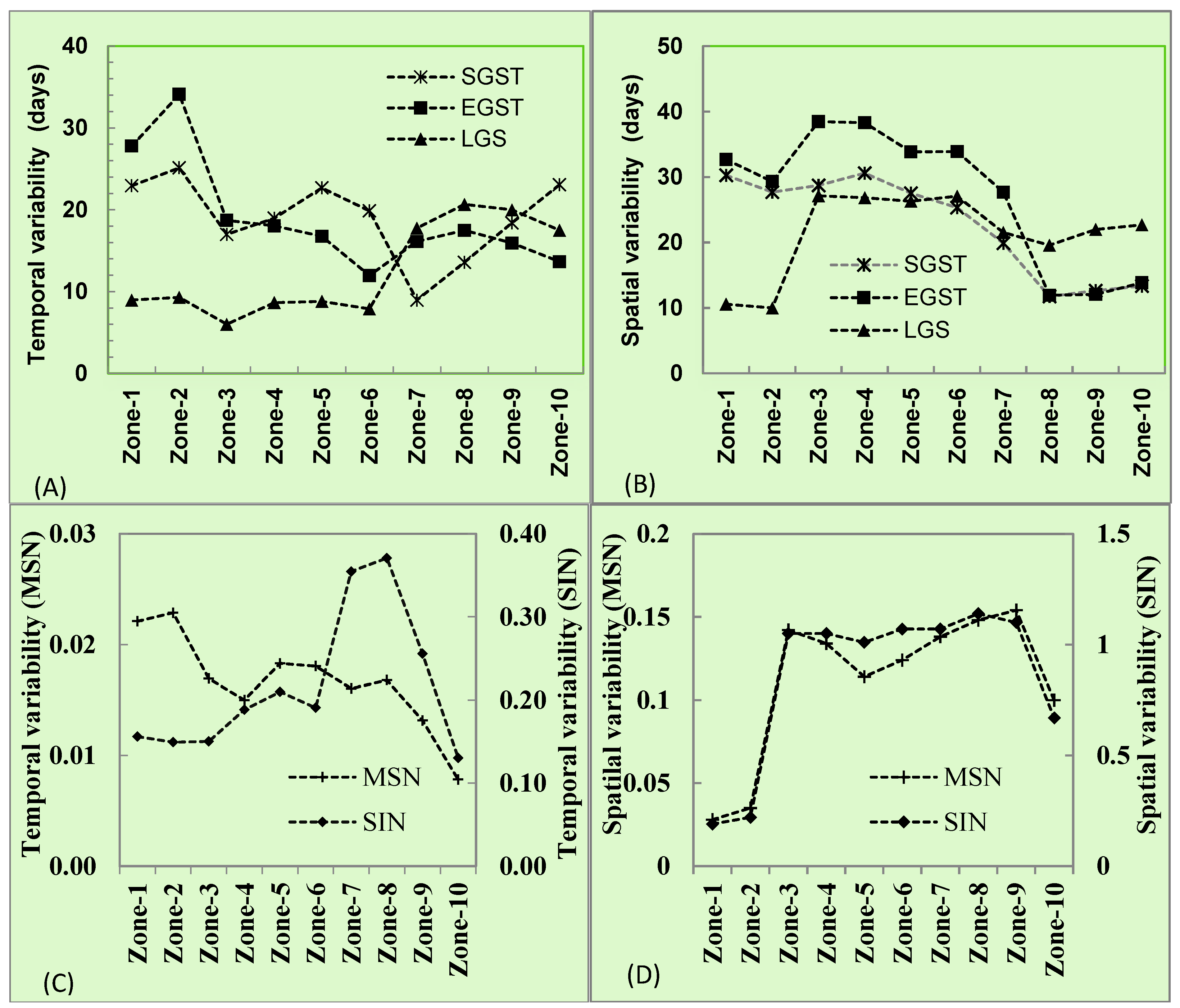
3.3. Phenology and Productivity Patterns

The 11-year means of the phenology metrics (including SGS, EGS, LGS) and productivity metrics (including MSN, SIN) were analysed across the elevation zones (Figure 4).

The earliest growing season found to start in the early days of MAM at TR (zone-3 to 6), in late days of MAM in HSR (zone-1 & 2) and then early days of JJA in high elevations (zone-7 to 10). The HSR was largely influenced by monsoon controlled rainfall and spring temperature regimes. The SGS was found retreating (late start) with rise in spring temperature (MAM) and advancing (early start) with increase in winter and spring rainfall. General late start of season observed in the HSR can be attributed to much less rainfall during the spring season in this region (Table 1 and Table 2) while vegetation growth is dependent on the moisture availability. In the rest of the regions, the SGS was found steadily shifting to later parts of the season with increase in elevation at higher elevation regions. The shift ranged from 144th day to 178th day with change in elevation from zone-7 to zone-8. The results show that SGS has different patterns across the bioclimatic regions.

The EGS ranges from August (240 DOY) to November (320 DOY). The difference in EGS by 80 days across elevation ranges clearly shows high variability compared to 64 days of SGS. The earliest and the latest end of the season occur at TR (zone-3) and highest elevations of AR (zone-10). The mid elevations, TR, which have not exhibited variation in SGS were found with increasing trend of EGST with rise of elevation. The range of variation was found by 27 days across the elevation zone-3 to zone-6. The higher elevations, SAR and AR, did not exhibit variation in EGST with increase in elevation as was found in case of SGS. The analysis shows that low and mid elevations have more EGS variability than high elevations.

Figure 4. Grassland phenology across elevation zones averaged over 11 years. Bars indicate start, end, and length of growing season—Grassland productivity patterns across the elevation zones as indicated by Maximum seasonal NDVI and seasonally integrated NDVI averaged over 11 years.

Figure 4. Grassland phenology across elevation zones averaged over 11 years. Bars indicate start, end, and length of growing season—Grassland productivity patterns across the elevation zones as indicated by Maximum seasonal NDVI and seasonally integrated NDVI averaged over 11 years.

The LGS was found with a range of 123–173 days across the bioclimatic regions. The increase in LGS was observed with rise in elevation till 3500 m (SAR) and then decline at further elevation in Alpine Regions. The maximum range of 150–173 days of LGS was found between elevation zone-6 to zone-7 (SAR) and lowest range of 120–123 days was found in lower elevations (HSR) where late SGS was observed due to limited moisture and early EGS was found due to rise in in-season temperature (JJA). The LGS was positively related with annual temperature (ANN_T), except temperate region, consequently contributing in overall grass productivity across the regions.

Table 1. Temperature across the elevation zones—average temperature in each zone with the spatial and temporal variability.

Elevation Zones	Temperature (°C)
	DJFT			MAMT			JJAT			SONT			ANNT
	µ	σs	σt	µ	σs	σt	µ	σs	σt	µ	σs	σt	µ	σs	σt
Zone 1	21.6	1.7	1.4	40.1	2.1	1.8	37.9	1.9	1.5	35.8	1.6	0.9	33.8	1.8	0.7
Zone 2	18.9	1.8	1.5	38.0	1.7	1.7	37.8	1.9	1.3	34.7	1.8	1.0	32.3	1.8	0.6
Zone 3	11.6	4.4	1.3	31.9	4.0	1.9	36.6	4.0	0.8	30.3	3.5	0.8	27.6	4.0	0.7
Zone 4	7.1	5.3	1.5	28.0	4.7	2.0	34.6	4.3	0.9	27.6	4.0	0.8	24.3	4.6	0.9
Zone 5	2.2	4.7	1.7	24.4	5.0	2.3	32.8	4.6	1.3	24.8	4.4	0.9	21.1	4.7	1.0
Zone-6	−1.0	4.6	1.6	20.5	6.1	2.3	29.5	5.9	1.4	21.6	4.9	0.9	17.7	5.4	1.0
Zone 7	−8.0	4.4	1.2	9.6	6.3	1.9	19.2	6.0	1.3	13.5	4.7	0.8	8.6	5.3	0.9
Zone 8	−11.1	3.5	1.1	5.8	4.1	1.9	17.2	3.8	1.7	11.7	3.5	0.7	5.9	3.7	0.9
Zone 9	−12.9	2.8	1.1	4.2	3.8	1.8	16.9	3.5	2.0	10.7	3.3	0.8	4.7	3.4	0.9
Zone 10	−14.1	2.7	0.9	3.7	4.2	1.7	16.1	3.7	2.0	8.9	3.3	0.8	3.7	3.5	0.9

µ = mean; σ_s = spatial standard deviation; σ_t = temporal standard deviation.

Table 1. Temperature across the elevation zones—average temperature in each zone with the spatial and temporal variability.

Elevation Zones	Temperature (°C)
	DJFT			MAMT			JJAT			SONT			ANNT
	µ	σs	σt	µ	σs	σt	µ	σs	σt	µ	σs	σt	µ	σs	σt
Zone 1	21.6	1.7	1.4	40.1	2.1	1.8	37.9	1.9	1.5	35.8	1.6	0.9	33.8	1.8	0.7
Zone 2	18.9	1.8	1.5	38.0	1.7	1.7	37.8	1.9	1.3	34.7	1.8	1.0	32.3	1.8	0.6
Zone 3	11.6	4.4	1.3	31.9	4.0	1.9	36.6	4.0	0.8	30.3	3.5	0.8	27.6	4.0	0.7
Zone 4	7.1	5.3	1.5	28.0	4.7	2.0	34.6	4.3	0.9	27.6	4.0	0.8	24.3	4.6	0.9
Zone 5	2.2	4.7	1.7	24.4	5.0	2.3	32.8	4.6	1.3	24.8	4.4	0.9	21.1	4.7	1.0
Zone-6	−1.0	4.6	1.6	20.5	6.1	2.3	29.5	5.9	1.4	21.6	4.9	0.9	17.7	5.4	1.0
Zone 7	−8.0	4.4	1.2	9.6	6.3	1.9	19.2	6.0	1.3	13.5	4.7	0.8	8.6	5.3	0.9
Zone 8	−11.1	3.5	1.1	5.8	4.1	1.9	17.2	3.8	1.7	11.7	3.5	0.7	5.9	3.7	0.9
Zone 9	−12.9	2.8	1.1	4.2	3.8	1.8	16.9	3.5	2.0	10.7	3.3	0.8	4.7	3.4	0.9
Zone 10	−14.1	2.7	0.9	3.7	4.2	1.7	16.1	3.7	2.0	8.9	3.3	0.8	3.7	3.5	0.9

µ = mean; σ_s = spatial standard deviation; σ_t = temporal standard deviation.

Table 2. Rainfall across the elevation zones—average temperature in each zone with the spatial and temporal variability.

Elevation Zones	Rainfall (mm)
	DJFR			MAMR			JJAR			SONR			ANNR
	µ	σs	σt	µ	σs	σt	µ	σs	σt	µ	σs	σt	µ	σs	σt
Zone 1	30.2	8.9	18.3	32.7	8.8	14	66.2	9.3	37.7	16.4	4.4	9.6	145.6	7.8	79.6
Zone 2	36.1	10	20.1	38.3	9.8	18.1	56	11.9	34.8	15.3	5.6	9.6	145.7	9.3	82.7
Zone 3	43.7	17.2	19	43.6	16.7	18.8	45.7	20.9	26.7	15.5	7	9.8	148.6	15.4	74.3
Zone 4	38.4	16.6	16.4	39.7	15.8	14.9	36.7	17.5	20.5	12.8	6	8.2	127.6	14	59.9
Zone 5	34.1	13.7	15.2	36	12.7	15.4	27.7	11.6	20.5	10.6	4.1	7.5	108.3	10.5	58.6
Zone 6	35.2	15.7	15.5	38.8	14.2	15.9	27.7	11.9	14.9	11.3	4.7	8.3	112.9	11.6	54.6
Zone 7	47.8	20.5	19.3	53	19	19.5	46.1	23.8	19.5	16.8	7.2	11.9	163.7	17.6	70.2
Zone 8	46.2	20	17.5	53	19.3	18.4	43.8	22.9	18.2	15.7	6.9	10.3	158.8	17.2	64.3
Zone 9	37.4	16.3	14.1	45.7	17.1	17.3	34.6	17.3	14.8	12.5	5.1	7.8	130.2	14	54.1
Zone 10	33	13.7	12.6	40.7	15.7	17.7	26.8	11.7	12.1	10.8	3.8	7	111.4	11.2	49.3

* DJF_T (mean seasonal temperature of winter), MAM_T (mean seasonal temperature of spring), JJA_T (mean seasonal temperature of summer), SON_T (mean seasonal temperature on autumn), ANN_T (Mean annual temperature), DJF_R (cumulative seasonal rainfall of winter), MAM_R (cumulative seasonal rainfall of spring), JJA_R (cumulative seasonal rainfall of summer), SON_R (cumulative seasonal rainfall of autumn) ANN_R (cumulative annual rainfall); Winter (December, January, February), spring (March, April, May), summer (June, July, August), autumn (September, October, November). µ = mean; σ_s = spatial standard deviation; σ_t = temporal standard deviation.

Table 2. Rainfall across the elevation zones—average temperature in each zone with the spatial and temporal variability.

Elevation Zones	Rainfall (mm)
	DJFR			MAMR			JJAR			SONR			ANNR
	µ	σs	σt	µ	σs	σt	µ	σs	σt	µ	σs	σt	µ	σs	σt
Zone 1	30.2	8.9	18.3	32.7	8.8	14	66.2	9.3	37.7	16.4	4.4	9.6	145.6	7.8	79.6
Zone 2	36.1	10	20.1	38.3	9.8	18.1	56	11.9	34.8	15.3	5.6	9.6	145.7	9.3	82.7
Zone 3	43.7	17.2	19	43.6	16.7	18.8	45.7	20.9	26.7	15.5	7	9.8	148.6	15.4	74.3
Zone 4	38.4	16.6	16.4	39.7	15.8	14.9	36.7	17.5	20.5	12.8	6	8.2	127.6	14	59.9
Zone 5	34.1	13.7	15.2	36	12.7	15.4	27.7	11.6	20.5	10.6	4.1	7.5	108.3	10.5	58.6
Zone 6	35.2	15.7	15.5	38.8	14.2	15.9	27.7	11.9	14.9	11.3	4.7	8.3	112.9	11.6	54.6
Zone 7	47.8	20.5	19.3	53	19	19.5	46.1	23.8	19.5	16.8	7.2	11.9	163.7	17.6	70.2
Zone 8	46.2	20	17.5	53	19.3	18.4	43.8	22.9	18.2	15.7	6.9	10.3	158.8	17.2	64.3
Zone 9	37.4	16.3	14.1	45.7	17.1	17.3	34.6	17.3	14.8	12.5	5.1	7.8	130.2	14	54.1
Zone 10	33	13.7	12.6	40.7	15.7	17.7	26.8	11.7	12.1	10.8	3.8	7	111.4	11.2	49.3

* DJF_T (mean seasonal temperature of winter), MAM_T (mean seasonal temperature of spring), JJA_T (mean seasonal temperature of summer), SON_T (mean seasonal temperature on autumn), ANN_T (Mean annual temperature), DJF_R (cumulative seasonal rainfall of winter), MAM_R (cumulative seasonal rainfall of spring), JJA_R (cumulative seasonal rainfall of summer), SON_R (cumulative seasonal rainfall of autumn) ANN_R (cumulative annual rainfall); Winter (December, January, February), spring (March, April, May), summer (June, July, August), autumn (September, October, November). µ = mean; σ_s = spatial standard deviation; σ_t = temporal standard deviation.

Overall, in terms of bioclimatic regions, the humid sub-tropical region has a late start, early end, and short growing season with low productivity; the temperate region has an early start, early end with moderate productivity that increases with elevation; the sub-alpine region has a late start, late end, and long growing season, with highest productivity; and the alpine region has a late start, early end, and short growing season with low productivity. The grass calendars as observed over the study areas broadly matches with ground-based reports [30,31].

In terms of variability across time (11 years) and space (within the bioclimatic regions), the SGS exhibits high spatial and temporal variability in the humid subtropical and alpine regions and low variability in the temperate and subalpine regions. The end of growing season had greater variability both in terms of days and in differences between bioclimatic regions, with a high temporal variability in the humid subtropical region and high spatial variability in all except the alpine region. The length of growing season also showed different spatial and temporal variability in the different bioclimatic regions, with a higher temporal variability in the subalpine and alpine regions, higher spatial variability in the temperate region, and low temporal and spatial variability in the humid subtropical region (Figure 5). The increase of SGS and decrease of EGS observed over different elevation regions of alpine zones and temperate zones respectively and also increase of LGS with rise in elevation reflects the possible control of climate across different elevations and growth stages of the grasses. Such characteristic variations of across elevation regions affecting grass calendars were also reported in the neighboring areas [28,32].

Figure 5. (A,B) Temporal and spatial variability of phenology calendar and (C,D) productivity patterns across the elevation zones. Temporal variability is the average temporal variance of the spatial mean of all pixels in each zone; spatial variability is the average spatial variance of the temporal mean of all pixels in each zone.

Figure 5. (A,B) Temporal and spatial variability of phenology calendar and (C,D) productivity patterns across the elevation zones. Temporal variability is the average temporal variance of the spatial mean of all pixels in each zone; spatial variability is the average spatial variance of the temporal mean of all pixels in each zone.

Seasonal maximum productivity, MSN, ranges from 0.15 (in zone-10) to 0.43 (in zone-7), whereas, integrated productivity ranges from 1.30 (in zone-1) to 3.25 (in zone-7). It was notable that LGS in zone-10 was higher than zone-1 but MSN in zone-10 was lower than that of zone-1, therefore, as a by product of MSN and LGS, SIN in elevation zone-1 was relatively higher than elevation zone-10. Analysis indicates that, HSR and AR were characterised with low productivity, TR were moderately productive, and SAR were highly productive. The maximum seasonal NDVI and seasonally integrated NDVI showed a similar pattern of change with elevation zone. Productivity increased with increase in elevation up to a maximum of 0.43 in sub-alpine region and decreased rapidly with elevation above 4000 masl (Alpine region) to a minimum of 0.15 at elevations above 4500 masl.

The maximum NDVI showed the highest temporal variability and lowest spatial variability in the humid subtropical region; temporal variability tended to decrease with elevation and spatial variability to increase, except at the highest elevation. Seasonally integrated NDVI showed low spatial and temporal variability in the humid subtropical region and in the highest zone of the alpine region; temporal variability was only high in the subalpine region, whereas spatial variability was high in the temperate, sub-alpine, and lower zone of the alpine region.

4. Discussion

The study was undertaken to support understanding of the climate controls on grassland phenology and productivity in the UIB basin using satellite-based information in absence of ground-based climate and vegetation data. The use of satellite based climatology data was helpful in understanding spatial patterns of seasonal and annual differences in rainfall (R_f) and temperature (T) in four bioclimatic regions—humid subtropical, temperate, subalpine, and alpine regions. Each zone showed diverse patterns of rainfall and temperature, the humid subtropical region had high rainfall, high temperature, and high rainfall variability, in three of the four seasons. The temperate region had medium rainfall and temperature with less variability between peak and lean seasons. The subalpine region had high rainfall and low temperature, with high variation in both rainfall and temperature. The alpine region had low temperature and rainfall, with lower variability. These spatio-temporal patterns of rainfall and temperature closely match with the observation made by [33] using ground based climate data across the elevation gradient of upper Indus basin. The role of climate on grassland calendars and production was assessed using these characteristics as a base. The analysis did not show any significant long-term climate trends except for the rainfall in the humid subtropical region over the 11-year time frame. The relationship between climatic patterns and grassland phenology was assessed in terms of the influence at different stages of grass growth and in the different bioclimatic regions.

Some significant relationships were identified based on 11 years of seasonal and annual climate phenology relations. In the low altitude humid subtropical region, the growing season was strongly related to preseason rainfall and temperature. The start of the growing season delayed (late) with higher preseason (spring) temperature and advanced (early) with higher preseason (winter, spring) rainfall; and the end of growing season advanced (early) with higher in-season (summer) temperature. This is in line with the fact that this region is largely influenced by monsoon rainfall and temperature regimes. The growing season started earliest overall in the temperate region instead of sub humid regions, which can be attributed to limited rainfall at the start of season and also the frequent moderate drought conditions in the sub-humid region [34]. A positive slope for the regression of phenology on autumn temperatures has been reported by several correlative analyses of plant time series [35,36]. The slopes identified may reflect chilling requirements, as the UniChill model assumes [37], and there is ample experimental evidence that a period of winter chilling brings budburst forward [38].

The temperate region start of season got delayed with higher preseason (winter) temperature even though grass productivity was not affected by seasonal or annual temperature or rainfall conditions in this region. This can be partly attributed to the good forest cover in the temperate zone, which reduces thermal effects and maintains soil moisture at the local scale. In the humid subtropical region, the productivity and seasonality do not have significant associations with annual temperature and annual rainfall, while it has strong association with seasonal climate conditions. The grass productivity in humid subtropical regions is moisture constrained where productivity increases with increase in summer rainfall. Similarly, seasonality of the grasses have a strong association with seasonal climate conditions where high spring temperature delays the start of season and increase in summer temperature retreats at the end of the season. The growing season in the subalpine and alpine regions starts early in case of higher preseason temperature in spring (MAM_T), which is probably due to snow melt triggering the grass growth. However, contribution of snow cover dynamics has not been investigated in the current study. The end of the growing season in the subalpine region was delayed with increased summer rainfall (JJA_R), and the growing season became longer consequently. The length of growing season was associated with temperature, especially annual temperature, in most zones, but in different ways in the different bioclimatic regions, with higher annual temperature associated with a longer growing season in the temperate, subalpine, and alpine regions, and with a shorter growing season in the humid subtropical region. The temperate region [39] showed that mean air temperature during late winter and spring, annual mean air temperature, and annual Growing Degree Days (GDD) totals have positive correlations with growing season duration.

No clear relationships were identified that were true for all parameters in all bioclimatic zones. This could be because the growth regime of grass is different in the different zones, and thus affected differently by changes. Equally, the failure to identify significant relationships, especially for the end of the growing season, could also be related to the use of seasonal averages to test for relationships. Seasonal minima for temperature and rainfall might be better indicators of temperature and moisture stress and show clearer relationships with the end of the growing season [40]. Overall, several significant relationships identified across bioclimatic regions show that the seasonality of grass has a strong association with seasonal climate conditions, with high spring temperatures advancing the start of the growing season in the sub alpine and alpine region and high summer temperatures leading to an earlier end to the growing season in the humid subtropical region. Further, annual mean temperature has a greater influence than annual precipitation on the grassland dynamics in the study area.

Other studies on long-term trends of climate change in the study area indicate possible impacts based on the grassland phenology and productivity behaviour observed in this study. Researchers observed in [41] a reduction in mean temperature during spring and summer and, as a result, a reduction in mean annual temperature in their analysis of ground data from 1966 to 2004 in the upper Indus basin. Our analysis suggests that start of growing season delays with lower spring temperatures and also productivity in the alpine and sub alpine areas is constrained by temperature. Thus the observed changes in the climate conditions in the recent past suggests that the alpine and sub-alpine grasslands were passing through a reduction in grassland productivity and a delay in the start of growing season. However, these historic trends may not persist in the long term future scenarios [42]. The climate–phenology relations observed in the current study are similar to other global and regional studies and [38] reported a link between length of growing season and temperature in Europe; they found that warming in spring by 1 °C advanced the growing season by seven days. In addition, authors in [39] reported an apparent increase in the mean annual growing season in Europe by 10.8 days from an analysis of satellite data from 1981 to 1991. The results of [43] also are consistent with data on the advance in the seasonal cycle (about seven days) which has been inferred from CO2 data taken between the 1960s and early 1990s [44]. A study on Tibetan Plateau also observed that the start of growth season (SOG) was delayed gradually, the end of growth season (EOG) advanced slowly, and the length of growth season (LOG) shortened gradually. The study also observed that elevation played an important role in the regional differentiation of phenology.

Grass productivity in the upper Indus basin was found to be rising with elevation to a maximum in the subalpine region. The high productivity in alpine zone is attributed to both seasonal amplitude (max plant growth/photosynthesis) and the extended length of the growing season in the zone. The higher biomass in the subalpine region in spring and summer as compared to the dry temperate or humid subtropical regions, is thought to reflect the increased soil moisture made available from snow melt during spring and early summer, which supports increased plant growth [45,46]. The study provides a basis for meaningful discussion on the development of local climate-vegetation models that can be used in grasslands management in the region [47]. More detailed analysis of production patterns would add further value for analysing the grazing potential. The information derived from this study can be integrated to assess grassland responses to climate variability and change and to support informed decision making for intra-annual and long term grazing management.

5. Conclusions

The observed correlations between climate factors, phenology, and productivity metrics should be seen as a first approximation using the best available data. The seasonal climatic parameters could potentially play a role as triggering, enhancing, or prohibitive factors that affect the start and/or end of the growing season. Spring temperature is the major determinant of the start of growing season in the alpine and sub-alpine region. The length of growing season is mostly being governed by the annual temperature all across the bioclimatic regions. The productivity (season integrated NDVI) is being influenced by summer and annual rainfall in the humid subtropical region, spring temperature in the alpine and sub-alpine region, and both temperature and rainfall are contributing in the temperate region.

In terms of implications for the transhumance grazing system, the large area of sub-alpine and alpine grasslands with higher LGS indicates the greater grazing potential. However, a high degree of temporal and spatial variability of LGS as observed in the study cautions for better ground-based understanding of the causes of variability and associated judicious planning needs for potential grazing. On the other hand, the humid subtropical zones occupying the second largest area with shorter LGS needs to be properly planned for grazing needs. The temperate zones covering the lowest proportion of grassland area but with a greater portion of the study area, supports grasses with early EGS and high variation in LGS across different elevations. The spatial information thus generated on crop calendars could be potentially used for spatial planning of grazing within the zone and regulating the grazing across the zones so as to sustainably meet the herd movements and grazing needs. Stochastically generated future projections can be potential future work to investigate long-term sustainability of grasslands in the region.

References

1. Harle, K.; Howden, S.; Hunt, L.; Dunlop, M. The potential impact of climate change on the Australian wool industry by 2030. Agric. Syst. 2007, 93, 61–89. [Google Scholar] [CrossRef]
2. Paudel, K.P.; Andersen, P. Assessing rangeland degradation using multi temporal satellite images and grazing pressure surface model in Upper Mustang, Trans Himalaya, Nepal. Remote Sens. Environ. 2010, 114, 1845–1855. [Google Scholar] [CrossRef]
3. Immerzeel, W.W.; Droogers, P.; de Jong, S.M.; Bierkens, M.F.P. Large-scale monitoring of snow cover and runoff simulation in Himalayan river basins using remote sensing. Remote Sens. Environ. 2009, 113, 40–49. [Google Scholar] [CrossRef]
4. Vetter, S. Rangelands at equilibrium and non-equilibrium: Recent developments in the debate. J. Arid Environ. 2005, 62, 321–341. [Google Scholar] [CrossRef]
5. Joshi, S.; Jasra, W.A.; Ismail, M.; Shrestha, R.M.; Yi, S.L.; Wu, N. Herders’ perceptions of and responses to climate change in northern pakistan. Environ. Manag. 2013, 52, 639–648. [Google Scholar] [CrossRef] [PubMed]
6. Tucker, C.J.; Sellers, P.J. Satellite remote sensing of primary production. Int. J. Remote Sens. 1986, 7, 1395–1416. [Google Scholar] [CrossRef]
7. Rigge, M.; Smart, A.; Wylie, B.; Gilmanov, T.; Johnson, P. Linking phenology and biomass productivity in South Dakota Mixed-Grass Prairie. Rangel. Ecol. Manag. 2013, 66, 579–587. [Google Scholar] [CrossRef]
8. Wang, J.; Rich, P.M.; Price, K.P.; Kettle, W.D. Relations between NDVI and tree productivity in the central Great Plains. Int. J. Remote Sens. 2004, 25, 3127–3138. [Google Scholar] [CrossRef]
9. Pettorelli, N.; Vik, J.O.; Mysterud, A.; Gaillard, J.M.; Tucker, C.J.; Stenseth, N.C. Using the satellite-derived NDVI to assess ecological responses to environmental change. Trends Ecol. Evol. 2005, 20, 503–510. [Google Scholar] [CrossRef] [PubMed]
10. Huete, A.; Didan, K.; Miura, T.; Rodriguez, E.; Gao, X.; Ferreira, L. Overview of the radiometric and biophysical performance of the MODIS vegetation indices. Remote Sens. Environ. 2002, 83, 195–213. [Google Scholar]
11. Thein, T.R.; Watson, F.G.R.; Cornish, S.S.; Anderson, T.N.; Newman, W.B.; Lockwood, R.E. Chapter 7 vegetation dynamics of Yellowstone’s Grazing System. Terr. Ecol. 2009, 7, 113–133. [Google Scholar]
12. Hangbin, Z.; Xiaoping, Y.; Jialin, L. MODIS data based NDVI Seasonal dynamics in agro-ecosystems of south bank Hangzhouwan bay. J. Agric. Res. 2011, 6, 4025–4033. [Google Scholar]
13. Martínez, B.; Gilabert, M.A. Vegetation dynamics from NDVI time series analysis using the wavelet transform. Remote Sens. Environ. 2009, 113, 1823–1842. [Google Scholar] [CrossRef]
14. Milesi, C.; Samanta, A.; Hashimoto, H.; Kumar, K.K.; Ganguly, S.; Thenkabail, P.S.; Srivastava, A.N.; Nemani, R.R.; Myneni, R.B. Decadal variations in NDVI and food production in India. Remote Sens. 2010, 2, 758–776. [Google Scholar] [CrossRef]
15. Xu, L.; Myneni, R.B.; Chapin, F.S., III; Callaghan, T.V.; Pinzon, J.E.; Tucker, C.J.; Zhu, Z.; Bi, J.; Ciais, P.; Tømmervik, H.; et al. Temperature and vegetation seasonality diminishment over northern lands. Nat. Clim. Chang. 2013, 3, 581–586. [Google Scholar] [CrossRef]
16. Bradley, B.A.; Jacob, R.W.; Hermance, J.F.; Mustard, J.F. A curve fitting procedure to derive inter-annual phenologies from time series of noisy satellite NDVI data. Remote Sens. Environ. 2007, 106, 137–145. [Google Scholar] [CrossRef]
17. Nemani, R.R.; Keeling, C.D.; Hashimoto, H.; Jolly, W.M.; Piper, S.C.; Tucker, C.J.; Myneni, R.B.; Running, S.W. Climate-driven increases in global terrestrial net primary production from 1982 to 1999. Science 2003, 300, 1560–1563. [Google Scholar] [CrossRef] [PubMed]
18. Potter, C.S.; Klooster, S.; Brooks, V. Interannual Variability in Terrestrial Net Primary Production: Exploration of Trends and Controls on Regional to Global Scales. Ecosystems 1999, 2, 36–48. [Google Scholar] [CrossRef]
19. Tucker, C.J.; Slayback, D.A.; Pinzon, J.E.; Los, S.O.; Myneni, R.B.; Taylor, M.G. Higher northern latitude normalized difference vegetation index and growing season trends from 1982 to 1999. Int. J. Biometeorol. 2001, 45, 184–190. [Google Scholar] [CrossRef] [PubMed]
20. Myneni, R.B.; Keeling, C.D.; Tucker, C.J.; Asrar, G.; Nemani, R.R. Increased plant growth in the northern high latitudes from 1981 to 1991. Nature 1997, 386, 698–702. [Google Scholar] [CrossRef]
21. Reed, B.; Brown, J. Measuring phenological variability from satellite imagery. J. Veg. Sci. 1994, 5, 703–714. [Google Scholar] [CrossRef]
22. Archer, D.R.; Fowler, H.J. Spatial and temporal variations in precipitation in the Upper Indus Basin, global teleconnections and hydrological implications. Hydrol. Earth Syst. Sci. 2004, 8, 47–61. [Google Scholar] [CrossRef]
23. Champion, G.H.; Seth, S.K. Forest Types of Pakistan; Pakistani Forest Institute: Peshawar, Pakistan, 1965; p. 233. [Google Scholar]
24. Butt, B.; Turner, M.D.; Singh, A.; Brottem, L. Use of MODIS NDVI to evaluate changing latitudinal gradients of rangeland phenology in Sudano-Sahelian West Africa. Remote Sens. Environ. 2011, 115, 3367–3376. [Google Scholar] [CrossRef]
25. White, M.; Running, S.; Thornton, P. The impact of growing-season length variability on carbon assimilation and evapotranspiration over 88 years in the eastern US deciduous forest. Int. J. Biometeorol. 1999, 42, 139–145. [Google Scholar] [CrossRef] [PubMed]
26. Cleland, E.E.; Chuine, I.; Menzel, A.; Mooney, H.A.; Schwartz, M.D. Shifting plant phenology in response to global change. Trends Ecol. Evol. 2007, 22, 357–365. [Google Scholar] [CrossRef] [PubMed]
27. Prince, S.D.; Goetz, S.J.; Goward, S.N. Monitoring primary production from Earth observing satellites. Water Air Soil Pollut. 1995, 82, 509–522. [Google Scholar] [CrossRef]
28. Kariyeva, J.; van Leeuwen, W.J.D. Environmental Drivers of NDVI-Based Vegetation Phenology in Central Asia. Remote Sens. 2011, 3, 203–246. [Google Scholar] [CrossRef]
29. Vrieling, A.; Beurs, K.M.; Brown, M.E. Variability of African farming systems from phenological analysis of NDVI time series. Clim. Chang. 2011, 109, 455–477. [Google Scholar] [CrossRef]
30. Kreutzmann, H. Pastoral Practices and Their Transformation in the North-Western. 2004, 8, 54–88. [Google Scholar] [CrossRef]
31. Nüsser, M.; Clemens, J. Impacts on mixed mountain agriculture in the Rupal Valley, Nanga Parbat, Northern Pakistan. Mountain Res. Dev. 2013, 16, 117–133. [Google Scholar] [CrossRef]
32. Liu, J.; Tan, X.; J, W.; Ma, J.; Zhang, N. Comparative analysis between the 2010 severe drought in southwest China and typical drought disasters. China Water Resour. 2011, 9, 17–20. [Google Scholar]
33. Palazzi, E.; Ahmad, T.; Paolo, C.; Elisa, V.; Antonello, P. Climatic characterization of Baltoro Glacier (Karakoram) and Northern Pakistan from in-situ stations. In Engineering Geology for Society and Territory; Lollino, G., Manconi, A., Clague, J., Shan, W., Chiarle, M., Eds.; Springer International Publishing: New York, NJ, USA, 2015; pp. 33–37. [Google Scholar]
34. Xie, H.; Ringler, C.; Zhu, T.; Waqas, A. Droughts in Pakistan: A spatiotemporal variability analysis using the Standardized Precipitation Index. Water Int. 2013, 38, 620–631. [Google Scholar] [CrossRef]
35. Fitter, A.; Fitter, R.; Harris, I.; Williamson, M. Relationships between first flowering date and temperature in the flora of a locality in central England. J. Func. Ecol. 1995, 296, 55–60. [Google Scholar] [CrossRef]
36. Cook, B.I.; Wolkovich, E.M.; Parmesan, C. Divergent responses to spring and winter warming drive community level flowering trends. Proc. Natl. Acad. Sci. USA 2012, 109, 9000–9005. [Google Scholar] [CrossRef] [PubMed]
37. Chuine, I. A unified model for budburst of trees. J. Theor. Biol. 2000, 207, 337–347. [Google Scholar] [CrossRef] [PubMed]
38. Laube, J.; Sparks, T.H.; Estrella, N.; Hofler, J.; Ankerst, D.P.; Menzel, A. Chilling outweighs photoperiod in preventing precocious spring development. Glob. Chang. Biol. 2014, 20, 170–182. [Google Scholar] [CrossRef] [PubMed]
39. Chen, X.; Pan, W. Relationships among phenological growing season, time-integrated normalized difference vegetation index and climate forcing in the temperate region of eastern China. Int. J. Climatol. 2002, 22, 1781–1792. [Google Scholar] [CrossRef]
40. Higuchi, K.; Worthy, D.; Chan, D.; Shahshkov, A. Regional source/sink impact on the diurnal, seasonal and inter-annual variations in atmospheric CO2 at a boreal forest site in Canada. Tellus 2003, 55, 115–125. [Google Scholar] [CrossRef]
41. Fowler, H.J.; Archer, D.R. Conflicting signals of climatic change in the upper Indus Basin. J. Clim. 2006, 19, 4276–4293. [Google Scholar] [CrossRef]
42. Milly, P.C.D.; Betancourt, J.; Falkenmark, M.; Hirsch, R.M.; Zbigniew, W.; Lettenmaier, D.P.; Stouffer, R.J. Stationarity is dead: Whither water management? Science 2008, 319, 573–574. [Google Scholar] [CrossRef] [PubMed]
43. Menzel, A.; Fabian, P. Growing season extended in Europe. Nature 1999. [Google Scholar] [CrossRef]
44. Ding, M.; Zhang, Y.; Sun, X.; Liu, L.; Wang, Z.; Bai, W. Spatiotemporal variation in alpine grassland phenology in the Qinghai-Tibetan Plateau from 1999 to 2009. Chin. Sci. Bull. 2013, 58, 396–405. [Google Scholar] [CrossRef]
45. Sardar, M.R. Indigenous Production and Utilization Systems in the High Altitude Alpine Pasture, Saif-ul- Maluk (NWFP), Pakistan; FAO and Pakistan Forest Institute: Peshawar, Pakistan, 1997. [Google Scholar]
46. Seth, C.M. Biomass fluctuation in alpine pastures of Kashmir Himalaya. Ann. Arid Zone 1996, 35, 65–67. [Google Scholar]
47. Chmielewski, F.-M.; Rötzer, T. Response of tree phenology to climate change across Europe. Agric. Forest Meteorol. 2001, 108, 101–112. [Google Scholar] [CrossRef]