
Assessing Potential Links between Climate Variability and Sea Levels along the Coasts of North America

 ,
,  ,
,
Abstract
:1. Introduction

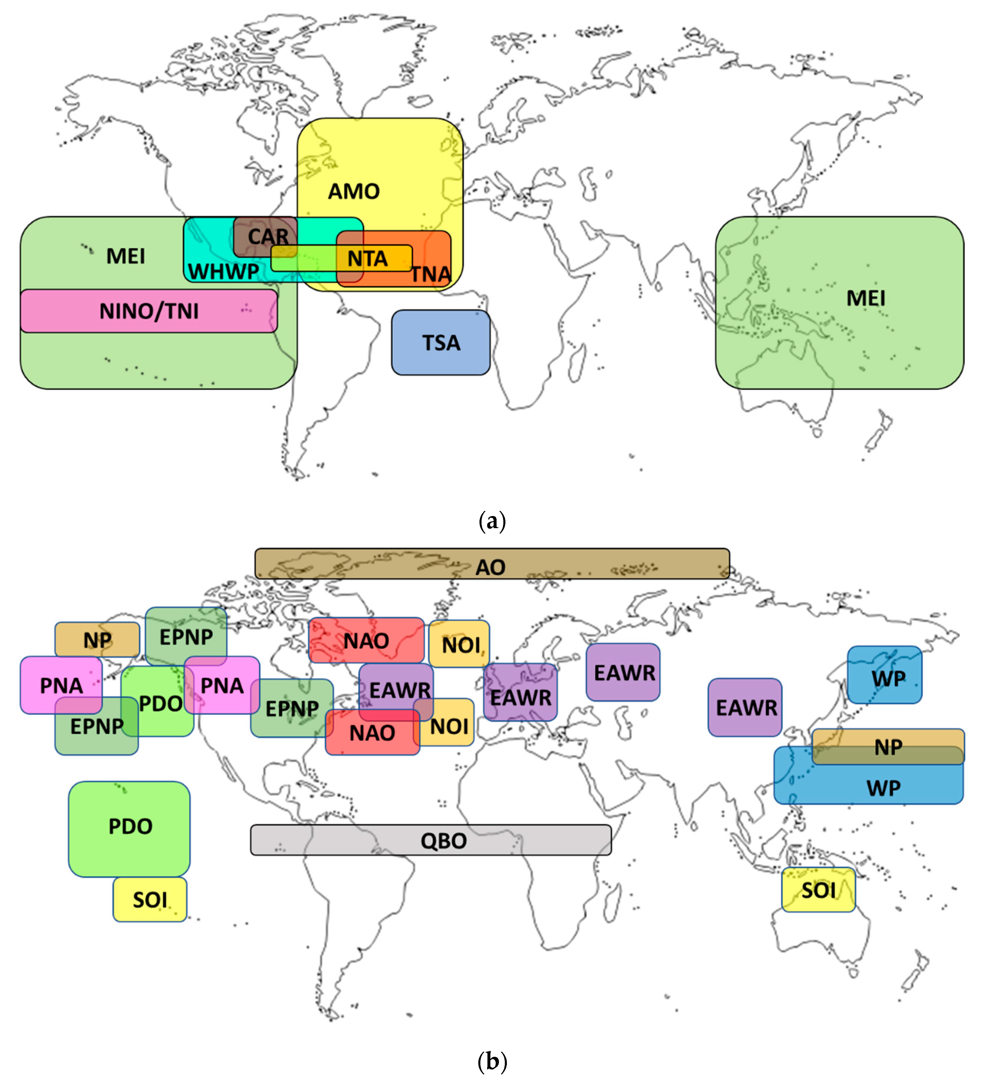
| CI (Abb.) | Climate Index | Beginning Year | Ending Year |
|---|---|---|---|
| AO | Arctic Oscillation | 1950 | 2018 |
| AMO | Atlantic Multidecadal Oscillation | 1948 | 2018 |
| CAR | Caribbean Index | 1950 | 2018 |
| EAWR | Eastern Asia/Western Russia | 1950 | 2013 |
| EPNP | East Pacific/North Pacific Oscillation | 1950 | 2018 |
| MEI | Multivariate ENSO Index | 1950 | 2018 |
| N12 | Niño 1 + 2 | 1950 | 2018 |
| N3 | Niño 3 | 1950 | 2018 |
| N34 | Niño 3.4 | 1950 | 2018 |
| N4 | Niño 4 | 1950 | 2018 |
| NAO | North Atlantic Oscillation | 1950 | 2018 |
| NP | North Pacific pattern | 1948 | 2018 |
| NTA | North Tropical Atlantic index | 1950 | 2018 |
| NOI | Northern Oscillation Index | 1948 | 2018 |
| PDO | Pacific Decadal Oscillation | 1948 | 2018 |
| PNA | Pacific North American index | 1950 | 2018 |
| QBO | Quasi-Biennial Oscillation | 1948 | 2018 |
| SOI | Southern Oscillation Index | 1951 | 2018 |
| TNI | Trans-Niño Index | 1948 | 2018 |
| TNA | Tropical Northern Atlantic index | 1948 | 2018 |
| TSA | Tropical Southern Atlantic index | 1948 | 2018 |
| WHWP | Western Hemisphere Warm Pool | 1948 | 2018 |
| WP | Western Pacific index | 1950 | 2018 |
2. Materials and Methods
2.1. Data
2.2. Method
3. Results
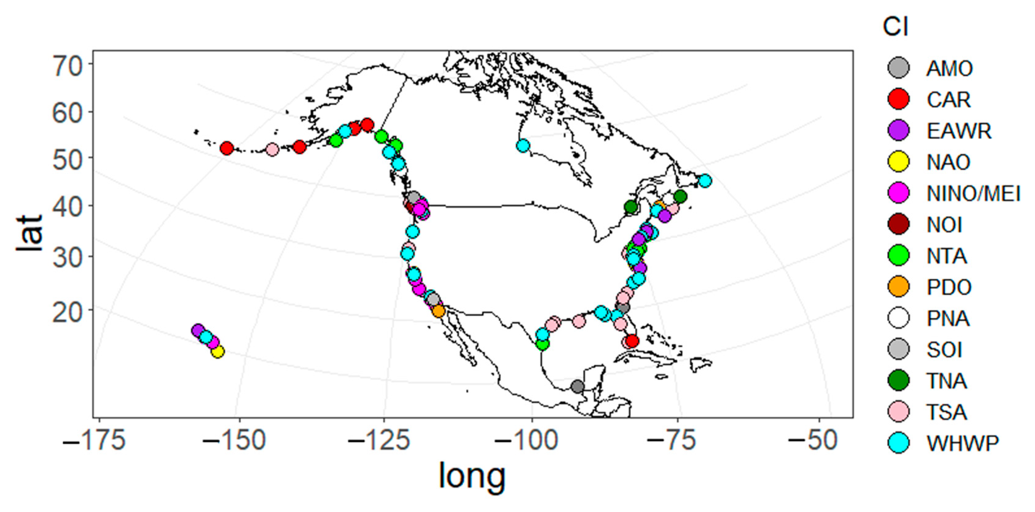
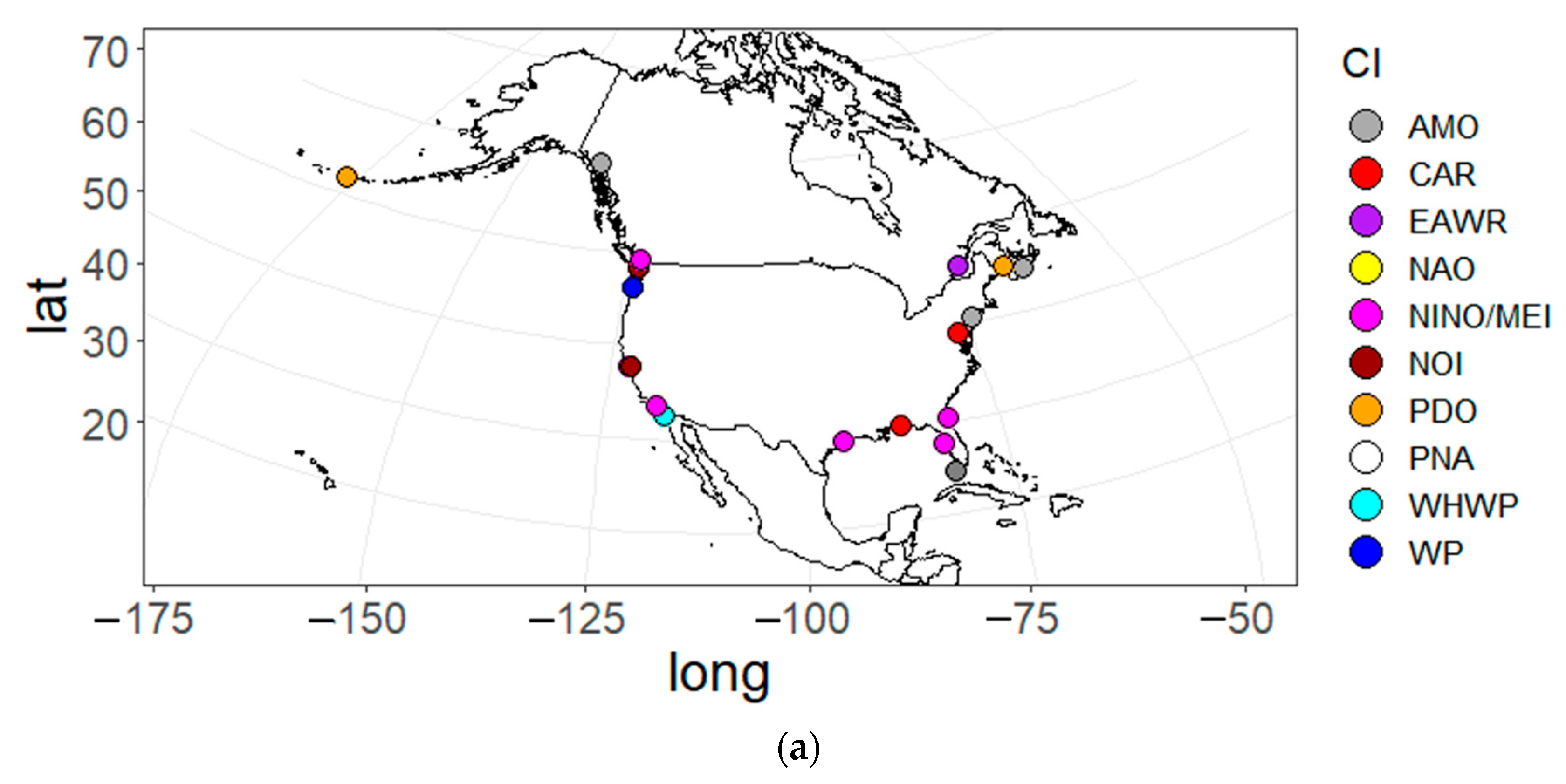
3.1. Multidecadal Coupling between the Coastal Sea Level and Different CIs
3.2. Coastal Sea Level Trend for Each Epoch
4. Discussion
5. Conclusions
Supplementary Materials
Author Contributions
Funding
Institutional Review Board Statement
Informed Consent Statement
Data Availability Statement
Acknowledgments
Conflicts of Interest
References
- World Bank. Building Resilience: Integrating Climate and Disaster Risk into Development; World Bank: Washington, DC, USA, 2013. [Google Scholar]
- Kelman, I.; Gaillard, J.C.; Mercer, J. Climate Change’s Role in Disaster Risk Reduction’s Future: Beyond Vulnerability and Resilience. Int. J. Disaster Risk Reduct. 2015, 6, 21–27. [Google Scholar] [CrossRef] [Green Version]
- Reguero, B.G.; Losada, I.J.; Díaz-Simal, P.; Méndez, F.J.; Beck, M.W. Effects of Climate Change on Exposure to Coastal Flooding in Latin America and the Caribbean. PLoS ONE 2015, 10, e0133409. [Google Scholar] [CrossRef] [PubMed]
- UNFPA (United Nations Fund for Population Activities). Linkages between Population Dynamics, Urbanization Processes and Disaster Risks: A Regional Vision of Latin America; UN-HABITAT, ISDR, UNFPA: New York, NY, USA, 2012. [Google Scholar]
- Cazenave, A.; Cozannet, G.L. Sea level rise and its coastal impacts. Earth’s Future 2014, 2, 15–34. [Google Scholar] [CrossRef]
- Church, J.A.; Clark, P.U.; Cazenave, A.; Gregory, J.M.; Jevrejeva, S.; Levermann, A.; Merrifield, M.A.; Milne, G.A.; Nerem, R.S.; Nunn, P.D.; et al. Sea level change. In Climate Change 2013: The Physical Science Basis. Contribution of Working Group I to the Fifth Assessment Report of the Intergovernmental Panel on Climate Change; Stocker, T.F., Qin, D., Plattner, G.-K., Tignor, M., Allen, S.K., Boschung, J., Nauels, A., Xia, Y., Bex, V., Midgley, P.M., Eds.; Cambridge University Press: Cambridge, UK; New York, NY, USA, 2013; pp. 1137–1216. [Google Scholar]
- Seneviratne, S.I.; Nicholls, N.; Easterling, D.; Goodess, C.M.; Kanae, S.; Kossin, J.; Luo, Y.; Marengo, J.; McInnes, K.; Rahimi, M.; et al. Changes in climate extremes and their impacts on the natural physical environment. In Managing the Risks of Extreme Events and Disasters to Advance Climate Change Adaptation. A Special Report of Working Groups I and II of the Intergovernmental Panel on Climate Change (IPCC); Field, C.B., Barros, V., Stocker, T.F., Qin, D., Dokken, D.J., Ebi, K.L., Mastrandrea, M.D., Mach, K.J., Plattner, G.-K., Allen, S.K., Tignor, M., Midgley, P.M., Eds.; Cambridge University Press: Cambridge, UK; New York, NY, USA, 2012; pp. 109–230. [Google Scholar]
- Merkens, J.-L.; Reimann, L.; Hinkel, J.; Vafeidis, A.T. Gridded population projections for the coastal zone under the Shared Socioeconomic Pathways. Glob. Planet. Chang. 2016, 145, 57–66. [Google Scholar] [CrossRef] [Green Version]
- Sallenger, A.H.; Doran, K.S.; Howd, P.A. Hotspot of accelerated sea-level rise on the Atlantic coast of North America. Nat. Clim. Chang. 2012, 2, 884–888. [Google Scholar] [CrossRef] [Green Version]
- Becker, M.; Karpytchev, M.; Papa, F. Hotspots of relative sea level rise in the tropics. In Tropical Extremes: Natural Variability and Trends; Venugopal, V., Sukhatme, J., Murtugudde, R., Roca, R., Eds.; Elsevier: Amsterdam, The Netherlands, 2019; pp. 203–262. [Google Scholar]
- Kirezci, E.; Young, I.R.; Ranasinghe, R.; Muis, S.; Nicholls, R.J.; Lincke, D.; Hinkel, J. Projections of global-scale extreme sea levels and resulting episodic coastal flooding over the 21st Century. Sci. Rep. 2020, 10, 11629. [Google Scholar] [CrossRef] [PubMed]
- Hauer, M.E.; Evans, J.M.; Mishra, D.R. Millions projected to be at risk from sea-level rise in the continental United States. Nat. Clim. Chang. 2016, 6, 691–695. [Google Scholar] [CrossRef]
- Nagy, G.J.; Gutiérrez, O.; Brugnoli, E.; Verocai, J.E.; Gómez-Erache, M.; Villamizar, A.; Olivares, I.; Azeiteiro, U.M.; Filho, W.L.; Amaro, N. Climate vulnerability, impacts and adaptation in Central and South America coastal áreas. Reg. Stud. Mar. Sci. 2019, 29, 100683. [Google Scholar] [CrossRef]
- Wong, P.P.; Losada, I.J.; Gattuso, J.-P.; Hinkel, J.; Khattabi, A.; McInnes, K.L.; Saito, Y.; Sallenger, A. Coastal systems and low-lying areas. In Climate Change 2014: Impacts, Adaptation and Vulnerability. Part A: Global and Sectoral Aspects. Working Group II. Contribution to the Fifth Assessment Report of the Intergovernmental Panel on Climate Change; Field, C.B., Barros, V.R., Dokken, D.J., Mach, K.J., Mastrandrea, M.D., Bilir, T.E., Chatterjee, M., Ebi, K.L., Estrada, Y.O., Genova, R.C., et al., Eds.; Cambridge University Press: Cambridge, UK, 2014; pp. 361–409. [Google Scholar]
- Watson, P.J. Acceleration in US mean sea level? A new insight using improved tools. J. Coast. Res. 2016, 32, 1247–1261. [Google Scholar] [CrossRef]
- Oppenheimer, M.; Glavovic, B.C.; Hinkel, J.; van de Wal, R.; Magnan, A.K.; Abd-Elgawad, A.; Cai, R.; Cifuentes-Jara, M.; DeConto, R.M.; Ghosh, T.; et al. Sea Level Rise and Implications for Low-Lying Islands, Coasts and Communities. In IPCC Special Report on the Ocean and Cryosphere in a Changing Climate; Pörtner, H.-O., Roberts, D.C., Masson-Delmotte, V., Zhai, P., Tignor, M., Poloczanska, E., Mintenbeck, K., Alegría, A., Nicolai, M., Okem, A., et al., Eds.; Cambridge University Press: Cambridge, UK; New York, NY, USA, 2019; pp. 321–445. [Google Scholar]
- Wallace, J.M.; Rasmusson, E.M.; Mitchell, T.P.; Kousky, V.E.; Sarachik, E.S.; von Storch, H.J. On the structure and evolution of ENSO-related climate variability in the tropical Pacific: Lessons from TOGA. Geophys. Res. 1998, 103, 14241–14259. [Google Scholar] [CrossRef]
- Merrifield, M.A.; Thompson, P.R. Interdecadal sea level variations in the Pacific: Distinctions between the tropics and extratropics. Geophys. Res. Lett. 2018, 45, 6604–6610. [Google Scholar] [CrossRef]
- Sweet, W.W.V.; Dusek, G.; Obeysekera, J.T.B.; Marra, J.J. NOAA Technical Report NOS CO-OPS 086: Patterns and Projections of High Tide Flooding along the US Coastline Using a Common Impact Threshold; National Oceanographic and Atmospheric Administration: Silver Spring, MD, USA, 2018. [Google Scholar]
- Khouakhi, A.; Villarini, G.; Zhang, W.; Slater, L.J. Seasonal predictability of high sea level frequency using ENSO patterns along the US West Coast. Adv. Water Resour. 2019, 131, 103377. [Google Scholar] [CrossRef]
- Bromirski, P.D.; Miller, A.J.; Flick, R.E.; Auad, G. Dynamical suppression of sea level rise along the Pacific coast of North America: Indications for imminent acceleration. J. Geophys. Res. Ocean. 2011, 116, C07005. [Google Scholar] [CrossRef] [Green Version]
- Moon, J.-H.; Song, Y.T.; Lee, H. PDO and ENSO modulations intensified decadal sea level variability in the tropical Pacific. J. Geophys. Res. Ocean. 2015, 120, 8229–8237. [Google Scholar] [CrossRef]
- Buckley, M.W.; Marshall, J. Observations, inferences, and mechanisms of Atlantic Meridional Overturning Circulation variability: A review. Rev. Geophys. 2016, 54, 5–63. [Google Scholar] [CrossRef] [Green Version]
- NOAA (National Oceanographic and Atmospheric Administration): Climate Indices: Monthly Atmospheric and Ocean Time Series. Available online: https://psl.noaa.gov/data/climateindices/list/ (accessed on 16 February 2016).
- Little, C.M.; Hu, A.; Hughes, C.W.; McCarthy, G.D.; Piecuch, C.G.; Ponte, R.M.; Thomas, M.D. The Relationship Between U.S. East Coast Sea Level and the Atlantic Meridional Overturning Circulation: A Review. Geophys. Res. Lett. 2019, 124, 6435–6458. [Google Scholar] [CrossRef] [PubMed] [Green Version]
- Smith, K.L.; Polvani, L.M. Modeling evidence for large, ENSO-driven interannual wintertime AMOC variability. Environ. Res. Lett. 2021, 16, 084038. [Google Scholar] [CrossRef]
- Hamlington, B.D.; Leben, R.R.; Kim, K.Y.; Nerem, R.S.; Atkinson, L.P.; Thompson, P.R. The effect of the El Nino-Southern Oscillation on US regional and coastal sea level. J. Geophys. Res. Ocean. 2015, 120, 3970–3986. [Google Scholar] [CrossRef] [Green Version]
- Kennedy, A.J.; Griffin, M.L.; Morey, S.L.; Smith, S.R.; O’Brien, J.J. Effects of El Niño–Southern Oscillation on sea level anomalies along the Gulf of Mexico coast. J. Geophys. Res. Ocean. 2007, 112, C05047. [Google Scholar] [CrossRef]
- Menéndez, M.; Woodworth, P.L. Changes in extreme high water levels based on a quasi-global tidegauge data set. J. Geophys. Res. Ocean. 2010, 115, C10011. [Google Scholar] [CrossRef] [Green Version]
- Muis, S.; Haigh, I.D.; Nobre, G.G.; Aerts, J.C.J.H.; Ward, P.J. Influence of El Niño–Southern Oscillation on global coastal flooding. Earths Future 2018, 6, 1311–1322. [Google Scholar] [CrossRef]
- Sweet, W.; Park, J. From the extreme to the mean: Acceleration and tipping points of coastal inundation from sea level rise. Earths Future 2014, 2, 579–600. [Google Scholar] [CrossRef]
- Hurrell, J.W. Decadal Trends in the North Atlantic Oscillation: Regional Temperatures and Precipitation. Science 1995, 269, 676–679. [Google Scholar] [CrossRef] [PubMed] [Green Version]
- Pinto, J.G.; Zacharias, S.; Fink, A.H.; Leckebusch, G.C.; Ulbrich, U. Factors contributing to the development of extreme North Atlantic cyclones and their relationship with the NAO. Clim. Dyn. 2009, 32, 711–737. [Google Scholar] [CrossRef] [Green Version]
- Kenigson, J.S.; Han, W.; Rajagopalan, B.; Yanto, M.; Jasinski, M. Decadal Shift of NAO-Linked Interannual Sea Level Variability along the US Northeast Coast. J. Clim. 2018, 31, 4981–4989. [Google Scholar] [CrossRef]
- Sweet, W.V.; Horton, R.; Kopp, R.E.; LeGrande, A.N.; Romanou, A. Sea level rise. In Climate Science Special Report: Fourth National Climate Assessment; Wuebbles, D.J., Fahey, D.W., Hibbard, K.A., Dokken, D.J., Stewart, B.C., Maycock, T.K., Eds.; USGCRP: Washington, DC, USA, 2017; Volume 1, pp. 333–363. [Google Scholar]
- Ezer, T.; Atkinson, L.P.; Corlett, W.B.; Blanco, J.L. Gulf Stream’s induced sea level rise and variability along the US mid-Atlantic coast. J. Geophys. Res. Ocean. 2013, 118, 685–697. [Google Scholar] [CrossRef] [Green Version]
- Wang, C.; Enfield, D.B. The Tropical Western Hemisphere Warm Pool. Geophys. Res. Lett. 2001, 28, 1635–1638. [Google Scholar] [CrossRef]
- Domingues, R.; Goni, G.; Baringer, M.; Volkov, D. What Caused the Accelerated Sea Level Changes Along the U.S. East Coast During 2010–2015? Geophys. Res. Lett. 2018, 45, 13367–13376. [Google Scholar] [CrossRef]
- Enfield, D.B.; Lee, S.K.; Wang, C. How are large western hemisphere warm pools formed? Prog. Oceanogr. 2006, 70, 346–365. [Google Scholar] [CrossRef]
- Volkov, D.L.; Baringer, M.; Smeed, D.; Johns, W.; Landerer, F.W. Teleconnection between the Atlantic Meridional Overturning Circulation and sea level in the Mediterranean Sea. J. Clim. 2019, 32, 935–955. [Google Scholar] [CrossRef] [Green Version]
- Fenoglio-Marc, L.; Tel, E. Coastal and global sea level change. J. Geodyn. 2010, 49, 151–160. [Google Scholar] [CrossRef]
- Wilcox, R. A note on the Theil-Sen regression estimator when the regressor is random and the error term is heteroscedastic. Biom. J. 1998, 40, 261–268. [Google Scholar] [CrossRef]
- Hünicke, B.; Zorita, E. Trends in the amplitude of Baltic Sea level annual cycle. Tellus A Dyn. Meteorol. Oceanogr. 2008, 60, 154–164. [Google Scholar] [CrossRef] [Green Version]
- Yue, S.; Wang, C. The Mann-Kendall test modified by effective sample size to detect trend in serially correlated hydrological series. Water Resour. Manag. 2004, 18, 201–218. [Google Scholar] [CrossRef]
- Hamed, K.H.; Rao, A.R. A modified Mann-Kendall trend test for autocorrelated data. J. Hydrol. 1998, 204, 182–196. [Google Scholar] [CrossRef]
- Joshi, N.; Kalra, A.; Thakur, B.; Lamb, K.W.; Bhandari, S. Analyzing the Effects of Short-Term Persistence and Shift in Sea Level Records along the US Coast. Hydrology 2021, 8, 17. [Google Scholar] [CrossRef]
- Aksoy, A.O. Investigation of sea level trends and the effect of the north Atlantic oscillation (NAO) on the black sea and the eastern Mediterranean Sea. Theor. Appl. Climatol. 2017, 129, 129–137. [Google Scholar] [CrossRef]
- Taibi, H.; Haddad, M. Estimating trends of the Mediterranean Sea level changes from tide gauge and satellite altimetry data (1993–2015). JOL 2019, 37, 1176–1185. [Google Scholar] [CrossRef]
- Lobeto, H.; Menéndez, M.; Losada, I.J. Toward a methodology for estimating coastal extreme sea levels from satellite altimetry. J. Geophys. Res. Ocean. 2018, 123, 8284–8298. [Google Scholar] [CrossRef] [Green Version]
- PSMSL (Permanent Service for Mean Sea Level): Tide Gauge Data. Available online: https://www.psmsl.org/data/ (accessed on 1 May 2020).
- Holgate, S.J.; Matthews, A.; Woodworth, P.L.; Rickards, L.J.; Tamisiea, M.E.; Bradshaw, E.; Foden, P.R.; Gordon, K.M.; Jevrejeva, S.; Pugh, J. New Data Systems and Products at the Permanent Service for Mean Sea Level. J. Coast. Res. 2012, 29, 493. [Google Scholar]
- IPCC. Climate Change 2021: The Physical Science Basis. Contribution of Working Group I to the Sixth Assessment Report of the Intergovernmental Panel on Climate Change; Masson-Delmotte, V., Zhai, P., Pirani, A., Connors, S.L., Péan, C., Berger, S., Caud, N., Chen, Y., Goldfarb, L., Gomis, M.I., et al., Eds.; Cambridge University Press: Cambridge, UK; New York, NY, USA, 2021. [Google Scholar]
- Giovannettone, J.P.; Zhang, Y. Identifying strong signals between low-frequency climate oscillations and annual precipitation using long-window correlation analysis. Int. J. Climatol. 2019, 39, 4883–4894. [Google Scholar] [CrossRef]
- Giovannettone, J.P.; Paredes-Trejo, F.; Barbosa, H.; dos Santos, C.A.C.; Kumar, T.V.L. Characterization of links between hydro-climate indices and long-term precipitation in Brazil using correlation analysis. Int. J. Climatol. 2020, 40, 5527–5541. [Google Scholar] [CrossRef]
- Giovannettone, J.P. Assessing the relationship between low-frequency oscillations of global hydro-climate indices and long-term precipitation throughout the United States. JAMC 2021, 60, 87–101. [Google Scholar]
- Efron, B. Estimating the error rate of a prediction rule: Improvement on cross-validation. JASA 1983, 78, 316–331. [Google Scholar] [CrossRef]
- Efron, B. Bootstrap methods: Another look at the jackknife. Ann. Stat. 1979, 7, 569–593. [Google Scholar] [CrossRef]
- Enfield, D.B.; Mestas-Nuñez, A.M.; Trimble, P.J. The Atlantic multidecadal oscillation and its relation to rainfall and river flows in the continental U.S. Geophys. Res. Lett. 2001, 28, 2077–2080. [Google Scholar] [CrossRef] [Green Version]
- Giovannettone, J.P. HydroMetriks—Climate Tool (Hydro-CLIM); HydroMetriks, LLC.: Silver Spring, MD, USA, 2020. [Google Scholar]
- Chambers, D.P.; Merrifield, M.A.; Nerem, R.S. Is there a 60-year oscillation in global mean sea level? Geophys. Res. Lett. 2012, 39, L18607. [Google Scholar] [CrossRef] [Green Version]
- Pan, H.; Lv, X. Is there a quasi 60-year oscillation in global tides? Cont. Shelf Res. 2021, 222, 104433. [Google Scholar] [CrossRef]
- Park, J.-H.; Kug, J.-S.; Li, T.; Behera, S.K. Predicting El Niño Beyond 1-year Lead: Effect of the Western Hemisphere Warm Pool. Sci. Rep. 2018, 8, 14957. [Google Scholar] [CrossRef] [Green Version]
- Cleveland, W.S. 1981 LOWESS: A program for smoothing scatter plots by robust locally weighted regression. Am. Stat. 1981, 35, 54. [Google Scholar] [CrossRef]
- Park, J.-H.; Kug, J.-S.; An, S.I.; Li, T. Role of the western hemisphere warm pool in climate variability over the western North Pacific. Clim. Dyn. 2019, 53, 2743–2755. [Google Scholar] [CrossRef]


| CI | % Sites | CI | % Sites | CI | % Sites | CI | % Sites |
|---|---|---|---|---|---|---|---|
| WHWP | 29.2 | NINO/MEI | 26.3 | NINO/TNI | 40.9 | WHWP | 36.2 |
| TSA | 17.7 | AMO | 15.8 | NOI | 13.6 | EAWR | 29.0 |
| NINO/MEI | 14.5 | EAWR | 10.5 | TNA | 13.6 | NINO/TNI | 8.7 |
| NTA/TNA | 13.6 | CAR | 10.5 | WHWP | 9.1 | WP | 8.7 |
| EAWR | 6.3 | PDO | 10.5 | WP | 9.1 | CAR | 7.2 |
| CAR | 5.2 | NOI | 10.5 | EAWR | 4.5 | PDO | 2.9 |
| NAO | 4.2 | PNA | 5.3 | NAO | 4.5 | NAO | 1.4 |
| PDO | 3.1 | WHWP | 5.3 | SOI | 4.5 | NOI | 1.4 |
| PNA | 2.1 | WP | 5.3 | NP | 1.4 | ||
| AMO | 1.0 | NTA | 1.4 | ||||
| NOI | 1.0 | SOI | 1.4 | ||||
| NP | 1.0 | ||||||
| SOI | 1.0 |
Disclaimer/Publisher’s Note: The statements, opinions and data contained in all publications are solely those of the individual author(s) and contributor(s) and not of MDPI and/or the editor(s). MDPI and/or the editor(s) disclaim responsibility for any injury to people or property resulting from any ideas, methods, instructions or products referred to in the content. |
© 2023 by the authors. Licensee MDPI, Basel, Switzerland. This article is an open access article distributed under the terms and conditions of the Creative Commons Attribution (CC BY) license (https://creativecommons.org/licenses/by/4.0/).
Share and Cite
Giovannettone, J.; Paredes-Trejo, F.; Amaro, V.E.; Santos, C.A.C.d. Assessing Potential Links between Climate Variability and Sea Levels along the Coasts of North America. Climate 2023, 11, 80. https://doi.org/10.3390/cli11040080
Giovannettone J, Paredes-Trejo F, Amaro VE, Santos CACd. Assessing Potential Links between Climate Variability and Sea Levels along the Coasts of North America. Climate. 2023; 11(4):80. https://doi.org/10.3390/cli11040080
Chicago/Turabian StyleGiovannettone, Jason, Franklin Paredes-Trejo, Venerando Eustáquio Amaro, and Carlos Antonio Costa dos Santos. 2023. "Assessing Potential Links between Climate Variability and Sea Levels along the Coasts of North America" Climate 11, no. 4: 80. https://doi.org/10.3390/cli11040080