Article

Brazil Wave Climate from a High-Resolution Wave Hindcast

1
Environmental Hydraulics Institute “IH Cantabria”, Universidad de Cantabria, 39011 Santander, Spain
2
IHE Delft, Department of Coastal, Urban Risk and Resilience, Westvest 7, 2611 Delft, The Netherlands
3
Instituto Dom Luiz (IDL), Faculdade de Ciências, Universidade de Lisboa, Campo Grande, 1749-016 Lisbon, Portugal
*
Author to whom correspondence should be addressed.
Climate 2022, 10(4), 53; https://doi.org/10.3390/cli10040053
Submission received: 26 February 2022 / Revised: 18 March 2022 / Accepted: 29 March 2022 / Published: 31 March 2022
(This article belongs to the Special Issue Wave Climate)

Abstract

:
A detailed climatology of ocean wind waves in the South Atlantic Ocean, based on ERA-5 reanalysis and in a higher-resolution wave hindcast (ERA-5H), both developed by the European Centre for Medium-Range Weather Forecasts, is presented. The higher resolution of the wave fields in the ERA-5H (22 km) allowed for a better description of the wind sea and swell features compared to previous global and regional studies along the Brazilian coast. Overall, it is shown that swell waves are more prevalent and carry more energy in the offshore area of the study area, while wind sea waves dominate the nearshore regions, especially along the northern coast of Brazil. The influence of different climate indices on the significant wave heights patterns is also presented, with two behavioral groups showing opposite correlations to the North Atlantic Oscillation and Southern Annular Mode than to the Southern Oscillation Index. The analysis of the decadal trends of wind sea and swell heights during the ERA-5H period (1979–2020) shows that the long-term trends of the total significant wave height in the South Atlantic Ocean are mostly due to swell events and the wave propagation effect from Southern Ocean storms.

1. Introduction

Waves result from the transfer of energy from the atmosphere to the ocean through the wind, therefore being closely related to variations in atmospheric regimes, which have higher temporal and spatial variability [1,2]. Two types of waves can be observed on the ocean’s surface: Wind sea and swell [3,4,5]. On the one hand, wind seas are short-period waves, generated by the overlaying winds, with a wave phase speed lower than the local wind speed. On the other hand, swells are long-period waves, generated afar, to a distance that can be thousands of kilometers away, with a wave phase speed that exceeds the local wind speed. Thus, when analyzing the wave climate, it is useful to divide the wave data into both wind sea climate and swell climate analyses [4,6,7], and any relationship with local winds must be established with caution.
Besides the wind sea and swell separation, waves are also analyzed regarding different wave parameters. These can be computed from the ocean wave spectrum, given that waves on the ocean surface can be interpreted as the sum of regular wave components with random phase angles and different frequencies. One of the most commonly used wave parameters is the significant wave height ( H s ), defined as the average height of the highest one-third of all the waves if computed from a wave record. Otherwise, when computed from wave spectra, H s = 4 m 0 , where m 0 is the zeroth spectral moment, computed as m 0 = 0 f 0 E ( θ , f ) , where E ( θ , f ) is the two-dimensional (2D) wave (variance) spectrum, and θ and f are the direction and the frequency, respectively. The 2D wave variance spectrum is related to the total energy content of the sea state [8]. The mean wave period ( T m ) can also be calculated from the wave spectrum, as well as the mean wave direction ( θ m ). Additionally, H s , T m , and θ m can also be computed separately for the wind sea and swell components of the sea state via partitioning of the wave spectrum, thus obtaining the wind sea and swell significant wave heights ( H s w and H s s , respectively), mean wave periods ( T m w and T m s ), and mean directions ( θ m w and θ m s ). Consider [4,7,9] for further details.
Since the wave climate is dominated by local and remote atmospheric conditions, it can also be analyzed regarding its temporal, directional, and spectral characteristics. These include the variability and periodicity of wave parameters and their association with climate indices [10]. Waves represent a key process within the climate system and can influence not only energy transfers between the ocean and the atmosphere but also heat and mass [11]. Thus, understanding the wave climate is important, for example, for monitoring of coastal erosion and sediment transport, coastal and offshore engineering, ship routing, environmental studies, and wave energy estimation for renewable energy purposes [12].
Given the potential impacts on coastal morphology and beach dynamics, extreme waves deserve special attention as part of the wave climate of a region, particularly in land-falling storms. Extreme wave events are responsible for the most drastic changes in coastal morphological evolution [13], frequently leading to extreme erosion processes. Moreover, understanding the patterns behind extreme waves is important for any coastal management and engineering activities, not to mention coastal hazard studies. These extreme wave heights are usually associated with storms, sometimes taking place far away [14]. Additionally, storm waves are often combined with storm surges, leading to severe effects in coastal zones [15]. For that matter, the assessment of the present wave climate is crucial to determine potential changes and trends, due to natural climate fluctuations, or anthropogenically induced climate change processes [4,16,17,18,19].
The most direct and obvious approach to studying wave climate is through observations. In situ wave measurements performed with oceanographic buoys represent the most realistic data, but they are local observations, geographically sparse, and limited [20,21]. On the other hand, even though remote sensing provides global coverage through satellite altimetry, it also represents a short time series (about 25 years) and low temporal and spatial resolution [22]. Therefore, numerical models are more often used and commonly applied to conduct wave climate studies, using reanalysis and hindcast data, where recent past wave events are simulated considering historical wind data in order to understand present wave climate [10]. The European Centre for Medium-Range Weather Forecasts (ECMWF) has a long tradition of producing reanalysis data. The ECMWF started atmospheric reanalysis in 1979 with the start of the satellite era. Up until the release of ERA-20C, ERA-Interim was the most complete ECMWF product. The evolution of forecast and hindcast methods eventually led to the development of ERA-5, which is the main dataset used in the present study.
A reanalysis relies on interpreting, relating, and combining different observations from multiple sources that document the evolution of the global atmosphere, ocean (including waves), land surface, cryosphere, and the carbon cycle. Equations of motion and physical processes are used to generate data products based on the assimilated information, which combine the first model result (short-range forecast) with observations (in the “analysis” step; [23]). The temporal consistency of the reanalysis depends on the quality of the input observations. These tools play an important role in improving observation systems through the feedback loop, which results from advances in data assimilation and the development of better forecast models. The improvement of forecasting systems is largely due to the evolution of observation systems over the last three decades, which is mainly a result of the advances in satellite technology [24,25].
Global wave climate studies including the South Atlantic Ocean (SAO) have been recently performed [4,11,26]. However, most wave climate studies are focused on the North Atlantic Ocean (NATL) [16,27,28,29]. Wave climate studies in the SAO are relatively limited, mostly regional, and lack long-term assessments (of more than 30 years). For instance, in Brazil, [30] studied the coast of Ceará in the north, and [31,32] analyzed the waves along the southern region in Santa Catarina and Rio Grande do Sul, respectively. The longest analyses in Brazil were performed by [33,34] in the southern region of the country, and by [35] in the southeast. Other authors, including [36,37], exemplify the few studies covering the entire Brazilian coast, based on reanalysis data. However, only the latter truly represents long-term analysis.
Considering the extension of the Brazilian coast, its wave climate is determined by winds originating in the SAO and the Southern Ocean, involving three large atmospheric systems: The SAO (including the respective Southern Ocean sector) extratropical storm belt, the Intertropical Convergence Zone (ITCZ), and the respective trade winds, from both hemispheres. Given these major mechanisms responsible for wave generation in the SAO, it can be concluded that the Brazilian coastline is influenced by two main wave systems: East-northeastern waves and south-southeastern waves [38]. The relevance of these atmospheric and wave systems across the coast of Brazil varies with the latitude and coastal orientation. Moreover, along the section between the southernmost region to the eastern region of the Brazilian coast, the austral winter months are the most energetic ones, whilst the most energetic period in the north region is from December to March, indicating different seasonality patterns along the study area.
The present study details, for the first time, the present wave climate across the entire coast of Brazil using wave data from an ECMWF high-resolution wave hindcast. This hindcast has been produced using ERA-5 reanalysis winds and sea ice concentration (SIC) and will henceforth be designated as ERA-5H. The goal of this study is to examine the wave climate variability and long-term trends along the coast of Brazil, based on the high-resolution ERA-5H hindcast, from 1979 to 2020.
The outline of this paper is as follows: Section 2 details the ERA-5 reanalysis and ERA-5H hindcast data, as well as in situ datasets, and a summary of the methodology used. The results and description of the wave climate off the coast of Brazil are presented in Section 3. Section 4 presents the key point analysis in which a comparison with in situ data was performed. Lastly, a summary of the study and concluding remarks are presented in Section 5.

2. Materials and Methods

2.1. The ECMWF ERA-5 Based Wave Hindcast

Reanalysis data are used for climate studies when there is a lack of observations. Due to the hectic nature of the atmosphere, models need constant updates in order to perform corrections to their results. Reanalyses use data assimilation to correct them by mixing observations and model simulations. On the other hand, the hindcast approach is based on running atmospheric and wave models for a historical period, but without data assimilation.
Produced with the purpose of replacing ERA-Interim, the ERA-5 reanalysis provides a comprehensive high-resolution record of the global atmosphere, land surface, and ocean wind waves from 1950 onwards. Meanwhile, ERA-5H is a long global wave model stand-alone run (i.e., not coupled) forced by ERA-5 hourly 10 m neutral winds, surface air density, gustiness, and SIC. Because no wave data assimilation was used with this hindcast, it can also be seen as a benchmark of the quality of ERA-5 atmospheric forcing.
Even though the outputs of both ERA-5 and ERA-5H are hourly, their horizontal resolution is very different, with the latter showing a higher resolution [39]. The horizontal resolution of ERA-5 is 31 km for the atmosphere and 40 km for the waves, while the ERA-5H wave resolution is 0.2° (22 km). Their spectral resolutions are also different, with ERA-5 showing 24 directions and 30 logarithmically spaced frequencies, while ERA-5H presents 36 directions and 36 frequencies. Moreover, ERA-5H uses a more recent global bathymetry, as presented in Table 1. Furthermore, ERA-5H was produced with ERA-5 winds and a modified version of the WAM wave model.
To better exemplify the differences between ERA-5 and ERA-5H, the spatial distributions of H s and wave energy flux ( P w ), as well as extreme wave conditions, in the study area are presented in the Supplementary Material. We should highlight the better performance of the ERA-5H, especially with the differences near the coast for extreme values of P w along the eastern region of Brazil.
To determine the wave climate variability along the coast of Brazil, several wave parameters were analyzed from 1979 to 2020, such as H s , T m , and θ m . However, when analyzing the entire Atlantic Ocean basin, wind speed ( U 10 ) and wind direction (φ) were examined based on ERA-5 data. while H s , and θ m were based on ERA-5H.

2.2. In Situ Wave Observations

The ERA-5H data were also compared against in situ wave observations. From all the buoy data available since 1979 along the coast of Brazil, 5 buoys from PNBOIA (Programa Nacional de Bóias) were selected. Table 2 presents the position of the buoys used in the evaluation and their respective ERA-5H grid points, which have similar coordinates. The ERA-5H grid points were chosen as the closest ERA-5H points to the actual location of the corresponding buoys they were intended to be compared to. The variables extracted from the buoys included H s , T m , and U 10 .

2.3. Methods

In order to better understand swell events in the region under study, a swell-tracking algorithm [40,41,42] was applied. With this, it was possible not only to quantify the events at different points of the coast but also to determine where they are coming from in order to evaluate the contribution of different storm generation areas.
The relationship between large-scale atmospheric forcing and the climatological variability of H s was studied through spatial correlation analysis, based on Pearson correlation, against the climate patterns most representative over the SAO. The patterns included the North Atlantic Oscillation (NAO), the El Nino Southern Oscillation (ENSO) represented by the Southern Oscillation Index (SOI), and the Southern Annular Mode (SAM).
The evaluation of how well ERA-5H represents the wave climate of Brazil was determined by comparing the ERA-5H hindcast (y) against in situ observations (x). This was performed with the construction of scatter plots, as well as the computation of statistic parameters as described below.
BIAS represents the deviation between two variables, which can be defined as the difference between the averages of the time series:
B I A S = s u m ( y x ) / l e n g t h ( x ) .
The Root Mean Square Error (RMSE) measures the difference between an estimated value and the true value:
R M S E = 1 N Σ i = 1 N ( x i y i ) 2 .
The linear regression slope, or symmetric slope (SS), describes how much one can expect Y to change as X increases. In an ideal situation, SS = 1.
S S = y ¯ x ¯ .
The Pearson correlation coefficient (ρ) is the measurement of how the two variables are related to each other, with 1 (−1) indicating a perfect correlation (anticorrelation).
ρ = Σ i = 1 N ( x i y ¯ ) 2 Σ i = 1 N ( y i x i ) 2 + ( x i y ¯ i ) 2 .
The scatter index (SI) is the measurement of the dispersion with regard to the line x = y (ideal).
S I = R M S E x ¯ 100 .
Finally, the intra-annual variability of wave parameters was examined for the same 5 key points used in the in situ observation analysis through monthly averages. The same points were used in the long-term variability analysis, but rather with linear trends of H s , H s w , and H s s .
A summary of the methodology applied is presented in Figure 1.

3. The Wave Climate of Brazil

3.1. Atlantic Ocean Wind and Wave Climates

The climatological annual means of U 10 and φ, as well as H s and θ m , for the entire Atlantic Ocean, are shown in Figure 2 (ERA-5 reanalysis data). For both hemispheres, the extratropical regions present the highest values of U 10 and H s . In these regions, the yearly mean U 10 can reach up to 12 m/s, while the mean H s can be higher than 4 m. The lowest U 10 values can be found approximately where the centers of the respective semi-permanent anticyclone systems are located in each hemisphere (the Azores and the St. Helena High, respectively), and along the western coast of the African continent. Regarding the mean H s , the lowest values are found in the tropical and subtropical regions (the “swell pools”; [43]) as well as closer to the coasts. In fact, between the latitudes of 30° S and 30° N, the mean H s is lower than 2 m.

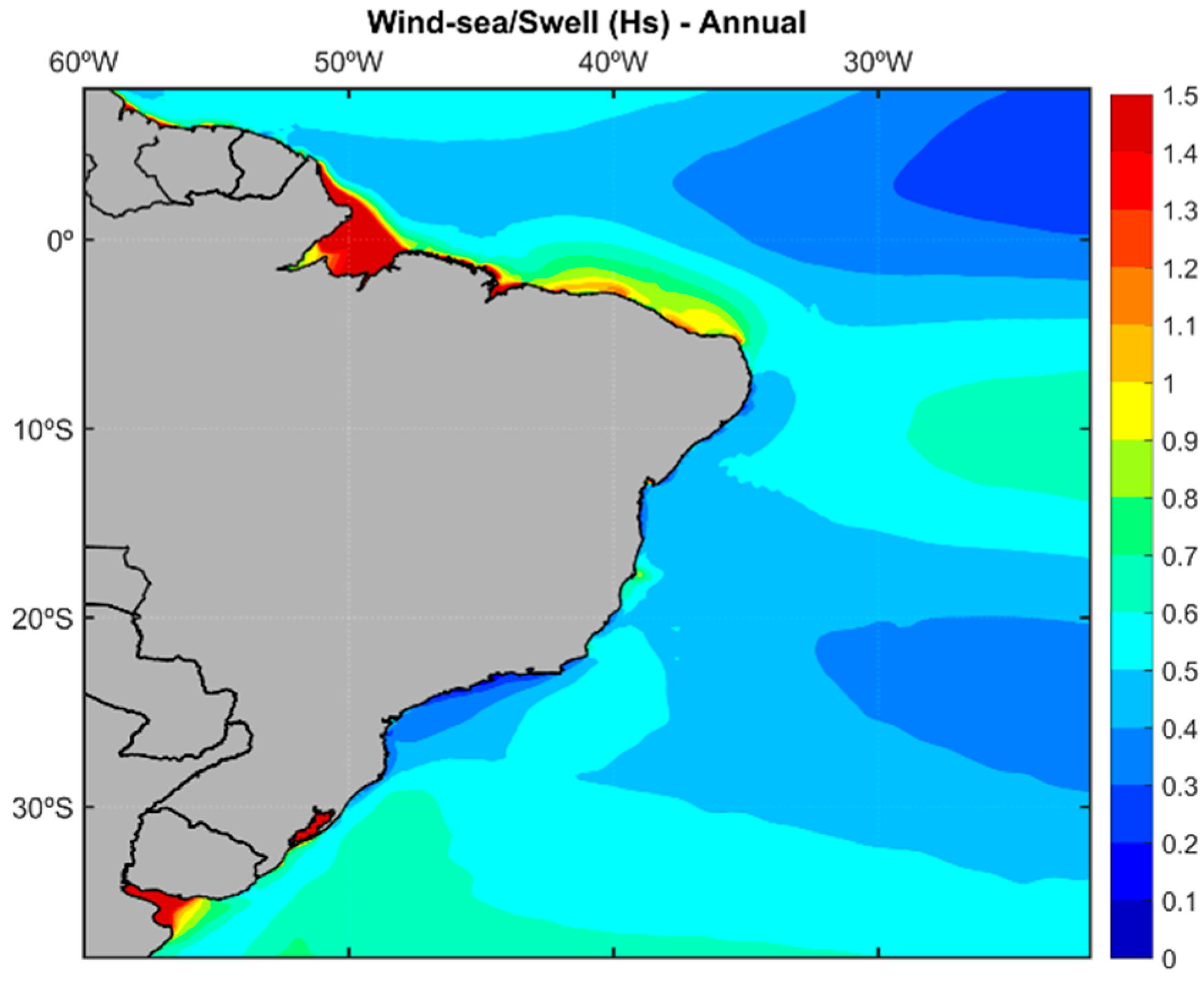
3.2. Brazil’s Mean Wave Heights and Directions (Wind Sea and Swell)

Figure 3 presents the climatological annual means of H s and θ m for the southwest Atlantic Ocean, along the coast of Brazil. Although most of the region shows H s around 1.75 m, it is possible to observe higher waves coming from the Southern Ocean as well as waves with H s higher than 2 m in the tropical SAO, approximately between 10° S and 20° S. Additionally, closer to the shore, waves tend to become smaller, mainly in enclosed areas, where there are major river mouths, which is the case for the Amazon River in the north of Brazil and the Rio de La Plata at the border between Argentina and Uruguay.
The distribution of the climatological annual means of H s w and θ m w , and H s s and θ m s , are shown in Figure 4. The differences between the wind sea- and swell-related parameters are easily noticeable. While the mean H s s reaches 2.5 m, with most of the offshore region ranging from 1.5 m and 1.75 m, the mean H s w does not exceed 1.5 m. Moreover, mean wave directions also differ between the two scenarios, with a larger contribution of SE and NE waves among the swell waves and E waves among the wind sea waves.
By dividing the climatological means of H s w by H s s , it is possible to observe the prevalence of wind sea or swell in the study area (Figure 5). Except for the north region of Brazil and the coast of Bahia along the eastern coast, the results indicate a swell predominance over wind sea waves, with values lower than 1. Moreover, the predominance of wind sea waves at the major river mouths is even clearer than in the annual H s results shown previously. Furthermore, the effect of the wind jets along the northern coast of Brazil is also more visible, with wind sea waves being almost as relevant as swell waves, which is represented by values around 1, indicating equal importance from both components. Areas closer to the coast indicate even higher values, representative of wind sea-dominated regions.

3.3. Extreme Wave Events

Extreme storm waves are characterized by uncommonly high wave heights. The extreme H s values were calculated as the 95th percentile (P95) [44]. Showing the climatological P95 results for the study area, Figure 6a reveals a latitudinal variation for most of the study area, from around 2 m in the tropical latitudes to more than 5 m in the subtropical SAO. Across the offshore area of Brazil, values between 2 m and 3.5 m are visible. However, the regions closer to the coast show values up to 2.5 m only. Accordingly, the maximum H s shown in Figure 6b also exhibits a decrease from the south of Brazil towards lower latitudes, with the lowest values in the equatorial region and the highest ones across the extra-tropical latitudes. Values above 10 m can only be found below 25° S and the entire north region of Brazil presents a maximum H s lower than 4 m, while the southeastern and eastern regions show values ranging from 4 m to 7 m.
In general, the extreme H s values in the study area are relatively low when compared to other regions of the world, such as the North Atlantic and North Pacific Oceans. Even higher latitudes of the SAO present higher extreme H s values than the Brazilian coast [45].

3.4. Wave Energy Flux

The wave energy flux (or the ability of the waves to perform work, in kw.m−1) is defined here as P w . The wave energy flux is a function of the wave periods and wave heights, to the first and second order, respectively [4]. Figure 7a displays the climatological annual means of P w for the coast of Brazil. Overall, with the exception of the extratropical region, P w is relatively low across the study area. However, higher values of wave power can be observed across the area where the most extreme waves were found. These waves most likely represent the edges of the Southern Ocean storm generation area.
Figure 7b shows the distribution of swell prevalence based on wave power by comparing P w w and P w s . The low values indicated in Figure 7b represent a higher predominance of P w s than P w w . This is a consequence of the fact that swell waves carry most of the ocean energy and are more regular than wind sea waves.
Additionally, the P w geographical distribution (Figure 7a) is similar to that of P95 (Figure 6a), with the lowest values closer to the shore and along the equatorial region and the highest values across the extra-tropical region. The influence of the coastal low-level wind jets along the north coast of Brazil can, once again, be observed when comparing the relationship between P w w and P w s (Figure 7b), with the local wind generating higher wind sea wave heights, closer to H s s .

3.5. Swell Events

Due to their dispersive properties, waves propagate freely away from their generation areas. Given similar conditions some waves might have as a result of the same generation storm, the waves tend to group themselves, constructing a swell event. These swell events can then be identified depending on the behavior of the peak wave period and peak mean wave direction. In order to isolate such events from the remaining local sea-state conditions, a swell-tracking algorithm was applied to 50 points along the coast of Brazil [40,41,42].
After choosing approximately equally distanced points along the coast of Brazil, the swell identification algorithm identified all individual swell events (from ERA-5H) that occurred at each of the coastal positions. Figure 8 displays the climatological annual mean number of swell events at each location, with a minimum of 0 events and a maximum of 12 events per year. Note that these values correspond to specific (pure) swell events that fill the criteria used in the algorithm. It is possible to observe that almost the entire north region of Brazil has an annual average of less than six swell events per year. On the other hand, the south and southeast regions range between 0.1 and 9 events, and the highest values are found along the east and northeast regions.
As mentioned, besides identifying and counting the swell events at each location, the swell-tracking algorithm can also estimate the approximate origin location and time of such events. Table A1 in Appendix A displays the results and coordinates for all 50 points selected for this analysis. To exemplify the results, 6 points were chosen from the original 50 points, and their results are presented in Table 3, which displays the contribution of multiple generation areas to the percentage of swell events coming from each section of the Atlantic Ocean basin. The southern points (4 and 11; Figure 8) indicate the SAO as being responsible for most of the swell events arriving in the region, while over 80% of the swell events arriving on the points in the northeast and north regions (31, 37, and 45) originate in the NATL. In addition, even though almost 72% of the events arriving at the eastern region (point 22) originated from storms in the SAO, over 10% originated in the Tropical Atlantic Ocean (TAO), possibly related to tropical cyclone activity.
Furthermore, none of the selected six points have the full 100% of their swell events formed in the Atlantic Ocean (Table 3). For instance, point 22 has the lowest percentage of Atlantic swells with 85%, out of which 13.3% originated in the TAO and 71.7% in the SAO. On the other hand, point 45 displays the highest percentage of Atlantic swell (98.4%), almost entirely originating in the NATL (97.6%). This result indicates that the Brazilian coast receives swell waves from other regions of the global ocean, such as the South Pacific and South Indian oceans.

3.6. Large Scale Atmospheric Forcing

Several studies have shown the possibility of wave climate variability being associated with atmospheric oscillations and modes, usually depicted as climate indices. The relevance of these events on wave climate has been proven by the control NAO has over H s of the NATL [16,46,47]. The NAO is the principal mode of sea-level pressure (SLP) variability in the NATL. The spatial pattern of the NAO consists of a dipole structure between the Azores’ high-pressure system and the Icelandic low-pressure system. During the positive phase of the NAO, the oscillation represented in this mode consists of a strong anticyclone over the Azores, extending its crest along the subtropical latitudes of the NATL and promoting free zonal circulation (storm belt), generally above 40° N. This, in turn, leads to strong westerly winds along the middle latitudes, generating bigger waves [16]. As a result, the wave generation processes in the NATL are influenced and, consequently, so are the swells arriving in Brazil.
Through a positive correlation, the results in Figure 9a show that a positive NAO value would be associated with the increase in H s along part of the northern coast of Brazil as a result of higher H s values in the NATL, propagating southwards as swell. However, most of the H s values in the study area are negatively correlated with NAO, pointing to a decrease in H s along the eastern and south-eastern coasts of Brazil during the positive NAO phase. Previous research [16] also concluded this by determining that latitudes off the storm areas, such as most of the study area, are subject to waves that are smaller than normal during the positive phase of NAO due to a narrower directional window of wind and waves.
The second climate mode analyzed in this study is the ENSO, which is a global phenomenon with a marked interannual variability. Even though this mode is centered in the equatorial Pacific Ocean, its influence has been proven globally. Moreover, ENSO is indirectly influenced by changes in global temperature and climate change [48]. For instance, previous authors [49] showed that the Atlantic Ocean can affect ENSO by influencing tropical circulation. For example, when the ascending branch of the Walker circulation is strengthened in the Atlantic Ocean, there is an associated stronger descending branch in the Pacific Ocean resulting in ocean surface divergence and, consequently, the development of La Niña.
The most common index to represent ENSO is the SOI. While a positive SOI value is representative of La Niña events, a negative SOI value corresponds to El Niño phases. Most of the Brazilian coast indicates an increase in H s during positive phases of ENSO, as shown by the positive correlations in Figure 9b. The results here agree with [50], who concluded that, during El Niño years, there is a reduction in H s of up to 8 cm in the northwest part of the SAO.
However, as the results showed, the offshore region of the south and southeast coasts of Brazil showed no correlation against SOI. This possibly happens because, during the negative SOI phase, there is an intensification of the subtropical jets blocking cold fronts traveling from higher latitudes, leading to a decrease in the incidence of S-SW waves, representative of regional storm waves and swell waves, which typically have a higher H s values [35,51].
The SAM is the leading variability mode affecting the Southern Hemisphere (SH) atmospheric circulation, responsible for approximately 30% of the climate variability in the region [18,22]. A positive SAM value is associated with weaker westerlies from 30° S to 50° S and stronger westerlies from 50° S to 70° S in the storm belt over the Southern Ocean. This dipole suggests that during positive SAM periods, extreme wave conditions are favored in the higher latitudes of the SH. However, given the compression of the Subantarctic Front during positive SAM periods with the storm belt contracting towards Antarctica [52], even though the associated waves are higher than average, they have to travel further to reach Brazil, thus losing some of their energy and, consequently, decreasing in height, as shown by the negative correlations in Figure 9c.

4. Key Points Analysis

4.1. In Situ vs. ERA-5H Analysis

The results of the evaluation of ERA-5H performance compared to in situ observations ( H s ), are illustrated in Figure 10. The scatterplots compare the in situ measurements with selected key points from the ERA-5H H s . The buoys and their respective key points have similar coordinates. The ERA-5H grid points were chosen as the closest ones to the actual location of the corresponding buoys they were intended to be compared to. In addition to the scatter plots, linear regression fits were computed, as well as the bias, RMSE, correlation coefficient (r), and SI. All statistics are overlaid on the scatter plots.
The correlation coefficients show an acceptable relationship between the modeled and observed H s , with values above 0.70 for all locations, with the highest correlations in Santos and Rio Grande (0.93 and 0.91, respectively) and the lowest in Porto Seguro (0.70). Overall, ERA-5H shows a slight overestimation of H s in Fortaleza, Recife, and Porto Seguro, but it underestimates H s in Santos and Rio Grande.
All locations showed RMSE values below 0.4, indicating that ERA-5H can represent the observed H s climate with reasonable accuracy. Moreover, although all five cases show similar scatter indexes, the SI results indicate that ERA-5H has the most similar H s to the Fortaleza buoy (12.64%) and that it differs the most from the waves recorded in Porto Seguro (24.61%).

4.2. Intra-Annual Variability

Figure 11 displays the intra-annual variability (monthly averages) of U 10 , H s , H s w and H s w , and T m , T m w and T m w , at the five key points selected for the buoy analysis.
The results show latitudinal variation with stronger seasonality in the equatorial region. Most of the variables follow the same pattern with higher values during the austral winter when the most powerful waves occur, propagated from the extratropical SAO. However, P1 stands out for the opposite seasonality signals when comparing wind sea and swell conditions, with the former always following the wind behavior. Regarding H s , while all points show higher values of H s s than H s w for every month, P1 displays the opposite from July to October, coinciding with the period of stronger winds as well. Furthermore, unlike the other locations, in P1, it is noticeable that some of the variables show their highest values from November to March (Figure 11a).
The different seasonality shown at P1 could be associated with the fact that the wave climate in the north region of Brazil responds directly to the ITCZ behavior and is highly influenced by atmospheric and marine climates of the Northern Hemisphere (NH). As the ITCZ moves southward in the austral summer, waves from the NH can reach the north coast of Brazil as a result of the northeasterly trade winds and more intense storm activity creating swell events [53].
The southern points (P4 and P5, Figure 11d,e) are under the influence of polar front systems and seasonal oscillations of the intensity and position of the St. Helena High. The same can be concluded in the central points (P2 and P3, Figure 11b,c) but to a lower extent [54]. Additionally, cold fronts in Brazil are more frequent during the austral winter, as described by [38], which could explain the most energetic waves during this period in the southern region. In contrast, in the northern region, the extreme wave conditions are mostly driven by the NH’s circumstances [54,55].
Moreover, intra-annual variability of the wave climate off the coast of Brazil can be analyzed through seasonal spatial distributions of H s and T m as well as monthly anomalies of H s , all of which can be found in the Supplementary Material.

4.3. Inter-Annual Variability and Trends

An inter-annual variability and trend analysis was performed for H s , H s w , and H s s at the five key points. Consistent positive H s trends from 1979 to 2020 can be seen at all key points, indicating that wave heights increased along the coast of Brazil during this period (Figure 12, Table 4).
Regarding H s and H s s , P5 presented the highest rates (3.4 cm.dec−1 and 2.5 cm.dec−1, respectively). On the other hand, for H s w , P2 showed the highest rate (3.2 cm.dec−1). P4 presented the lowest rates for all three parameters analyzed.
Most of the Brazilian coast presented a higher rate for H s w than for H s s , except for P4 and P5 located in the southeast and south regions, respectively. This indicates a possible increase in the local wind over the central and northern points of the coast. The importance of local wind and wind sea waves along the northern coast has been pointed out previously in this study. Furthermore, the positive trend of H s s along the southern regions could be an indication of increased wind speed in the storm generation areas of the SAO.
Regarding the positive trends in the northern and central sectors, these could be associated with an increase in storm activity in the NH [56]. In contrast, the increase in H s along the southern regions may have been associated with the SAM positive trend since the 1960s [18,57], although the present study indicated a negative correlation between H s and SAM in this region. However, because the present correlation analysis did not isolate swell waves or winter conditions, the possible influence of the SAM positive trend could have been masked by wind sea waves and summer conditions.
The increase in H s over the last four decades, observed in the present study, was also noted in the NATL [16,28], and a shift from a negative to a positive H s trend in the 1990s was detected in Italy [27]. Several hypotheses have been raised to explain it, such as interannual and inter-decadal variabilities, long-term trends driven by global climate change, storm activities, and greenhouse gas concentrations [29]. Moreover, several studies have discussed the possibility of the upward trend from the mid-1960s and 1970s being associated with the improvement of aerial observations and the beginning of the satellite era around the same period. This would be due to the fact that, as a result, the development of both the monitoring and understanding of wind and atmospheric pressure occurred, essential for wave studies in general [24,58].
Furthermore, an increase in sea surface temperature (SST) as a result of climate change may be leading to an increase in wave energy, implying an increase in either wave height or period, or even both. By statistically comparing global wave energy flux and SST, previous authors [59] found a significant positive correlation between the two, as well as a positive trend of the former of 0.4% per year since 1948. The authors based their conclusion on the fact that wind waves respond to the wind regime, which, in turn, is critically influenced by SST.

5. Conclusions

A qualitative analysis of the wave climate off the coast of Brazil, from the high-resolution ECMWF global hindcast ERA-5H, has been presented here. The higher temporal and geographical resolutions of ERA-5H, when compared to other wave hindcasts and reanalyses, allowed a better representation and understanding of the wave climate of the SAO.
The analysis was performed for wind sea and swell waves separately, as well as for the total sea-state wave conditions. It has been shown that the wind sea and swell characteristics in the SAO agree with the global knowledge that swell waves are higher, more energetic, and more prevalent in the open ocean than wind sea waves [4,43,60].
Extreme wave events and wave energy content were examined through extreme wave heights (P95), maximum wave heights, and wave power (wave energy flux). All three variables presented a similar geographical distribution, with the lowest values closer to the shore and along the equatorial region and the highest ones across the extra-tropical region, which most likely represent the edges of the Southern Ocean storm generation area.
Because of the propagation effect of the waves, changes in H s are most likely related to changes in the conditions of the storm generation areas rather than a direct response to changes in regional wind speed. Thus, an examination of the swell events arriving at the coast of Brazil was performed to better understand where such waves are coming from. The results showed that even though the study area is sheltered from the Indian and Pacific Oceans, not all swell events originate in the Atlantic Ocean. For instance, as we move towards the central region of Brazil, the contribution of Atlantic swells decreases to approximately 75%, as opposed to the 85% of Atlantic swells detected in the northern and southern regions. These results indicate that the Indian and Pacific Oceans also have a relevant contribution and should be considered in studies involving the impact of climate forcing and climate change over the wave climate of the SAO.
Still, given the high contribution of the Atlantic Ocean in the study area, the influence of large-scale atmospheric circulation patterns on the H s climate was investigated through correlations with the NAO, SOI, and SAM indices. Although at different levels, both the NAO and the SAM were shown to have a negative correlation with most of the study area, apart from the most northern region. Yet, the values were all very low. On the other hand, SOI was shown to have relatively higher positive correlation values across the entire offshore tropical area and the northern region of the coast. It also showed a positive correlation with the central region, although at a lower level.
It should be pointed out that similar studies compute this correlation by separating winter and summer conditions [50]. However, in the present study, the entire time series was considered, which could lead to inaccurate results since certain climate modes peak at different periods of the year.
The ERA-5H H s data were also compared against in situ data from five different buoys along the coast of Brazil. The results showed an underestimation of H s along the southern regions of the study area, where the correlation coefficients were also the highest between observed and modelled data.
Past studies have outlined such behavior regarding ERA-5. For instance, previous research [61] detected an underestimation (overestimation) of H s in swell-dominated areas (wind sea-dominated areas). Here, ERA-5H seems to be moving in the same direction, underestimating H s in the southernmost locations. These areas were also described as swell-dominated regions in the present study. On the other hand, an overestimation of H s along the northern coast of Brazil has been shown. This area has been described here as a wind-sea-dominated region.
The long-term variability of the significant wind sea and swell wave heights was investigated separately to assess how they combine to influence the long-term trends of the H s in the SAO. The upward trend of H s observed here could be a result of the intensification of the westerlies along the SH projected for the 21st century as described by [62]. According to the authors, this mechanism would lead to an increase in the climatological extreme wave heights, such as maximum H s , as a result of the poleward shift of extratropical storms. This process is also represented by the significant trend toward the positive phase of SAM since the mid-1960s [18,57]. Another supporting result for such an assumption is the latitudinal variation of the H s s trends shown in the present study, with the highest rates at higher latitudes.
For a clearer view of the wave conditions in the area and how these might change under a climate change scenario, further studies are needed, involving the inter-relationships of different climate modes as well as different storm generation areas.

Supplementary Materials

The following supporting information can be downloaded at: https://www.mdpi.com/article/10.3390/cli10040053/s1, Figure S1. Spatial distribution of annual averages of H s (m) (a), P95 (m) (c), P w (Kw) (e) and P95 of P w (Kw) (g) based on ERA5, for Brazil. Spatial distribution of annual averages of H s (m) (b), P95 (m) (d), P w (Kw) (f) and P95 of P w (Kw) (h) based on ERA-5H, for Brazil; Figure S2: Spatial distribution of seasonal averages of H s (m) and θ m (°) for (a) DJF, (b) MAM, (c) JJA, and (d) SON, for Brazil; Figure S3: Spatial distribution of seasonal averages of T m (s) and θ m (°) for (a) DJF, (b) MAM, (c) JJA, and (d) SON for Brazil; Figure S4: Spatial distribution of H s anomalies (m) per month for Brazil.

Author Contributions

Conceptualization, A.S.; methodology, A.S. and G.L.; software, C.S.C. and G.L.; formal analysis, C.S.C.; investigation, C.S.C.; data curation, G.L.; writing—original draft preparation, C.S.C.; writing—review and editing, C.S.C., A.S. and G.L.; visualization, C.S.C.; supervision, A.S. All authors have read and agreed to the published version of the manuscript.

Funding

Gil Lemos acknowledges funding from Fundação para a Ciência e a Tecnologia (FCT), Grant FCT—UIDB/50019/2020—IDL.

Data Availability Statement

ERA-5 data can be downloaded from this website: https://cds.climate.copernicus.eu/cdsapp#!/dataset/reanalysis-era5-pressure-levels?tab=overview (accessed on 22 March 2021). ERA5-H is a new hindcast dataset under production; data are available on reasonable request. Observational (in situ) buoy data can be downloaded from this website: https://www.marinha.mil.br/chm/dados-do-goos-brasil/pnboia-mapa (accessed on 8 June 2021).

Conflicts of Interest

The authors declare no conflict of interest.

Appendix A

In this appendix, the results of the swell-tracking algorithm analysis for the entire coast of Brazil are displayed.
Table A1. Coordinates of the points used in the swell-event analysis and their respective annual mean number of swell events, total number of swell events, and percentages of swells (%) coming from each storm-originating area in the Atlantic Ocean: North Atlantic Ocean (NATL), Tropical Atlantic Ocean (TAO), and South Atlantic Ocean (SAO).
PointsCoordinatesSwell EventsSwell Origin Areas (%)
LatitudeLongitudeYearly AverageTotalNATLTAOSAOAtlantic Ocean
1−34−53.25.42260.00.981.982.7
2−33−52.27.02940.00.784.485.0
3−32−51.47.12990.00.789.089.6
4−31−50.47.33060.00.789.590.2
5−30−49.85.72380.00.488.288.7
6−29−495.02100.01.085.286.2
7−28−48.45.42280.05.381.686.8
8−27−48.26.32650.06.878.585.3
9−26−48.27.43110.03.983.987.8
10−25.2−47.47.23040.04.379.984.2
11−24.6−46.62.81160.07.486.894.1
12−24.2−45.68.53560.06.279.285.4
13−23.6−44.21.5620.025.845.271.0
14−23.4−42.81.9810.017.350.667.9
15−23−41.62.3960.019.854.274.0
16−22−40.83.11290.010.159.769.8
17−21−40.44.82000.06.073.079.0
18−20−39.87.02940.04.168.072.1
19−19−39.48.03380.02.768.070.7
20−18−3910.74480.00.469.269.6
21−17−38.811.95010.00.666.767.3
22−16−38.61.4600.013.371.785.0
23−15−38.610.04180.03.361.564.8
24−14−38.46.82850.013.052.665.6
25−13.4−381.7710.012.743.756.3
26−12.6−37.60.62615.47.719.242.3
27−11.8−371.56471.910.90.082.8
28−10.8−36.26.326485.20.80.086.0
29−10−35.63.615288.80.00.088.8
30−9−353.213590.40.00.090.4
31−8−34.64.117487.90.60.088.5
32−7−34.69.539982.50.50.083.0
33−6−34.81.9780.06.476.983.3
34−5−35.28.837186.50.00.086.5
35−4.6−36.65.924687.80.80.088.6
36−4−37.63.414292.30.70.093.0
37−3.4−38.43.816189.42.50.091.9
38−2.8−39.22.912196.71.70.098.3
39−2.4−40.42.410097.02.00.099.0
40−2.2−41.80.27100.00.00.0100.0
41−2−430.000.00.00.00.0
42−1.4−44.22.29186.80.00.086.8
43−0.8−45.62.19098.90.00.098.9
44−0.4−46.62.61100.05.583.689.1
450−47.83.012697.60.80.098.4
460.4−48.82.81190.05.976.582.4
471−49.43.01240.03.280.683.9
482−49.83.91640.04.980.585.4
493−50.63.71570.05.780.386.0
504−50.84.51910.02.674.377.0

References

  1. Cuchiara, D.C.; Fernandes, E.H.; Strauch, J.C.; Calliari, L.J. Modelagem Numérica do Comportamento das Ondas na Costa do Rio Grande do Sul. In Proceedings of the II Seminário e Workshop em Engenharia Oceânica, Rio Grande, Brazil, 23–25 November 2006. [Google Scholar]
  2. Sempreviva, A.M.; Schiano, M.E.; Pensieri, S.; Semedo, A.; Tomé, R.; Bozzano, R.; Borghini, M.; Grasso, F.; Soerensen, L.L.; Teixeira, J.; et al. Observed development of the vertical structure of the marine boundary layer during the LASIE experiment in the Ligurian Sea. Ann. Geophys. 2010, 28, 17–25. [Google Scholar] [CrossRef] [Green Version]
  3. Stewart, R.H. Introduction to Physical Oceanography; Department of Oceanography, Texas A&M University: College Station, TX, USA, 2005; p. 353. [Google Scholar] [CrossRef]
  4. Semedo, A.; Suselj, K.; Rutgersson, A.; Sterl, A. A Global View on the Wind Sea and Swell Climate and Variability from ERA-40. J. Clim. 2011, 24, 1461–1479. [Google Scholar] [CrossRef]
  5. Rutgersson, A.; Sætra, Ø.; Semedo, A.; Carlsson, B.; Kumar, R. Impact of surface waves in a Regional Climate Model. Meteorol. Z. 2010, 19, 247–257. [Google Scholar] [CrossRef]
  6. Holthuijsen, L.H. Waves in Oceanic and Coastal Waters; Cambridge University Press: New York, NY, USA, 2007; p. 405. [Google Scholar]
  7. Carrasco, A.; Semedo, A.; Isachsen, P.E.; Christensen, K.H.; Saetra, Ø. Global surface wave drift climate from ERA-40: The contributions from wind-sea and swell. Ocean Dyn. 2014, 64, 1815–1829. [Google Scholar] [CrossRef]
  8. Hughes, S.A.; Miller, H.C. Transformation of Significant Wave Heights. J. Waterw. Port Coast. Ocean. Eng. 1987, 113, 588–605. [Google Scholar] [CrossRef]
  9. Semedo, A. Seasonal Variability of Wind Sea and Swell Waves Climate along the Canary Current: The Local Wind Effect. J. Mar. Sci. Eng. 2018, 6, 28. [Google Scholar] [CrossRef] [Green Version]
  10. Pecher, A.; Kofoed, J.P. Handbook of Ocean Wave Energy; Springer Open: Aalborg, Denmark, 2017; p. 305. [Google Scholar]
  11. Cavaleri, L.; Fox-Kemper, B.; Hemer, M. Wind Waves in the Coupled Climate System. Bull. Am. Meteorol. Soc. 2012, 93, 1651–1661. [Google Scholar] [CrossRef]
  12. WMO. World Meteorological Organization. Guide to Wave Analysis and Forecasting, 2nd ed.; World Meterological Organization WMO: Geneva, Switzerland, 1998; p. 168. [Google Scholar]
  13. Masselink, G.; Gehrels, R. Coastal Environments & Global Change; American Geophysical Union and John Wiley & Sons, Ltd: New York, NY, USA, 2014; pp. 299–335. Available online: www.wiley.com/go/masselink/coastal (accessed on 23 December 2019).
  14. Young, I.R. Seasonal variability of the global ocean wind and wave climate. Int. J. Climatol. 1999, 19, 931–950. [Google Scholar] [CrossRef]
  15. Marcos, M.; Rohmer, J.; Vousdoukas, M.I.; Mentaschi, L.; Le Cozannet, G.; Amores, A. Increased Extreme Coastal Water Levels Due to the Combined Action of Storm Surges and Wind Waves. Geophys. Res. Lett. 2019, 46, 4356–4364. [Google Scholar] [CrossRef] [Green Version]
  16. Dodet, G.; Bertin, X.; Taborda, R. Wave climate variability in the North-East Atlantic Ocean over the last six decades. Ocean Model. 2010, 31, 120–131. [Google Scholar] [CrossRef]
  17. Kumar, P.; Min, S.K.; Weller, E.; Lee, H.; Wang, X.L. Influence of climate variability on extreme ocean surface wave heights assessed from ERA-interim and ERA-20C. J. Clim. 2016, 29, 4031–4046. [Google Scholar] [CrossRef]
  18. Marshall, A.G.; Hemer, M.A.; Hendon, H.H.; McInnes, K.L. Southern annular mode impacts on global ocean surface waves. Ocean Model. 2018, 129, 58–74. [Google Scholar] [CrossRef]
  19. Lemos, G.; Semedo, A.; Dobrynin, M.; Behrens, A.; Staneva, J.; Bidlot, J.-R.; Miranda, P. Mid-twenty-first century global wave climate projections: Results from a dynamic CMIP5 based ensemble. Glob. Planet. Chang. 2019, 172, 69–87. [Google Scholar] [CrossRef]
  20. Menéndez, M.; Mendez, F.; Losada, I.; Graham, N.E. Variability of extreme wave heights in the northeast Pacific Ocean based on buoy measurements. Geophys. Res. Lett. 2008, 35. [Google Scholar] [CrossRef]
  21. Semedo, A.; Vettor, R.; Breivik, Ø.; Sterl, A.; Reistad, M.; Soares, C.G.; A Lima, D.C. The wind sea and swell waves climate in the Nordic seas. Ocean Dyn. 2014, 65, 223–240. [Google Scholar] [CrossRef]
  22. Hemer, M.A.; Church, J.A.; Hunter, J.R. Variability and trends in the directional wave climate of the Southern Hemisphere. Int. J. Clim. 2010, 30, 475–491. [Google Scholar] [CrossRef]
  23. Buizza, R.; Brönnimann, S.; Haimberger, L.; Laloyaux, P.; Martin, M.J.; Fuentes, M.; Alonso-Balmaseda, M.; Becker, A.; Blaschek, M.; Dahlgren, P.; et al. The EU-FP7 ERA-CLIM2 Project Contribution to Advancing Science and Production of Earth System Climate Reanalyses. Bull. Am. Meteorol. Soc. 2018, 99, 1003–1014. [Google Scholar] [CrossRef] [Green Version]
  24. Dee, D.P.; Balmaseda, M.A.; Balsamo, G.; Engelen, R.; Simmons, A.J.; Thépaut, J.-N. Toward a Consistent Reanalysis of the Climate System. Bull. Am. Meteorol. Soc. 2014, 95, 1235–1248. [Google Scholar] [CrossRef]
  25. Aarnes, O.J.; Abdalla, S.; Bidlot, J.-R.; Breivik, Ø. Marine Wind and Wave Height Trends at Different ERA-Interim Forecast Ranges. J. Clim. 2015, 28, 819–837. [Google Scholar] [CrossRef] [Green Version]
  26. Young, I.R.; Zieger, S.; Babanin, A.V. Global Trends in Wind Speed and Wave Height. Science 2011, 332, 451–455. [Google Scholar] [CrossRef]
  27. Martucci, G.; Carniel, S.; Chiggiato, J.; Sclavo, M.; Lionello, P.; Galati, M.B. Statistical trend analysis and extreme distribution of significant wave height from 1958 to 1999—An application to the Italian Seas. Ocean Sci. 2010, 6, 525–538. [Google Scholar] [CrossRef] [Green Version]
  28. Wang, X.L.; Feng, Y.; Swail, V.R. North Atlantic wave height trends as reconstructed from the 20th century reanalysis. Geophys. Res. Lett. 2012, 39, 1–6. [Google Scholar] [CrossRef]
  29. Bertin, X.; Prouteau, E.; Letetrel, C. A significant increase in wave height in the North Atlantic Ocean over the 20th century. Glob. Planet. Chang. 2013, 106, 77–83. [Google Scholar] [CrossRef]
  30. Moura, M.R. Aspectos Climáticos versus Variação Sazonal do Perfil Morfodinâmico das Praias do Litoral Oeste de Aquiraz, Ceará, Brasil. Rev. Bras. Climatol. 2012, 11, 208–222. [Google Scholar] [CrossRef] [Green Version]
  31. Araujo, C.E.S.; Franco, D.; Melo, E.; Pimenta, F. Wave Regime Characteristics of the Southern. In Proceedings of the International Conference on Coastal and Port Engineering in Developing Countries, COPEDEC VI, Colombo, Sri Lanka, 16–20 September 2003; Paper No. 097. p. 15. [Google Scholar]
  32. Sprovieri, F.C. Clima de Ondas, Potencial Energético e o Transporte de Sedimentos no Litoral Norte do Rio Grande do Sul. Ph.D. Thesis, Universidade Federal do Rio Grande do Sul, Porto Alegre, Brazil, 2018. [Google Scholar]
  33. Silva, P.G.; Klein, A.H.; Gonzalez, M.; Gutiérrez, O.Q.G.; Espejo, A. Performance assessment of the database downscaled ocean waves (DOW) on Santa Catarina coast, South Brazil. An. Acad. Bras. Cienc. 2015, 87, 623–634. [Google Scholar] [CrossRef] [Green Version]
  34. Oliveira, B.A.; Sobral, F.; Fetter, A.; Mendez, F.J. A high-resolution wave hindcast off Santa Catarina (Brazil) for identifying wave climate variability. Reg. Stud. Mar. Sci. 2019, 32, 100834. [Google Scholar] [CrossRef]
  35. Pereira, N.E.D.S.; Klumb-Oliveira, L.A. Analysis of the influence of ENSO phenomena on wave climate on the central coastal zone of Rio de Janeiro (Brazil). J. Integr. Coast. Zone Manag. 2015, 15, 353–370. [Google Scholar] [CrossRef] [Green Version]
  36. Pianca, C.; Mazzini, P.L.F.; Siegle, E. Brazilian offshore wave climate based on NWW3 reanalysis. Braz. J. Oceanogr. 2010, 58, 53–70. [Google Scholar] [CrossRef]
  37. Espindola, R.L.; Araújo, A.M. Wave energy resource of Brazil: An analysis from 35 years of ERA-Interim reanalysis data. PLoS ONE 2017, 12, e0183501. [Google Scholar] [CrossRef] [PubMed]
  38. Dominguez, J.M.L. The Coastal Zone of Brazil: An Overview. J. Coast. Res. 2013, 39, 16–20. [Google Scholar]
  39. Hersbach, H.; Bell, B.; Berrisford, P.; Hirahara, S.; Horanyi, A.; Muñoz-Sabater, J.; Nicolas, J.; Peubey, C.; Radu, R.; Schepers, D.; et al. The ERA5 global reanalysis. Q. J. R. Meteorol. Soc. 2020, 146, 1999–2049. [Google Scholar] [CrossRef]
  40. Portilla, J. Storm-Source-Locating Algorithm Based on the Dispersive Nature of Ocean Swells. Avances 2012, 4, C22–C36. [Google Scholar]
  41. Amores, A.; Marcos, M. Ocean Swells along the Global Coastlines and Their Climate Projections for the Twenty-First Century. J. Clim. 2020, 33, 185–199. [Google Scholar] [CrossRef]
  42. Lemos, G.; Semedo, A.; Hemer, M.; Menendez, M.; A Miranda, P.M. Remote climate change propagation across the oceans—The directional swell signature. Environ. Res. Lett. 2021, 16, 064080. [Google Scholar] [CrossRef]
  43. Chen, G.; Chapron, B.; Ezraty, R.; VanDeMark, D. A Global View of Swell and Wind Sea Climate in the Ocean by Satellite Altimeter and Scatterometer. J. Atmos. Ocean. Technol. 2002, 19, 1849–1859. [Google Scholar] [CrossRef]
  44. Campos, R.; Alves, J.-H.; Soares, C.G.; Guimaraes, L.; Parente, C.E. Extreme wind-wave modeling and analysis in the south Atlantic ocean. Ocean Model. 2018, 124, 75–93. [Google Scholar] [CrossRef]
  45. Barbariol, F.; Bidlot, J.; Cavaleri, L.; Sclavo, M.; Thomson, J.; Benetazzo, A. Maximum wave heights from global model reanalysis. Prog. Oceanogr. 2019, 175, 139–160. [Google Scholar] [CrossRef]
  46. Bacon, S.; Carter, D.J.T. A connection between mean wave height and atmospheric pressure gradient in the North Atlantic. Int. J. Clim. 1993, 13, 423–436. [Google Scholar] [CrossRef]
  47. Kushnir, Y.; Cardone, V.J.; Greenwood, J.G.; Cane, M.A. The Recent Increase in North Atlantic Wave Heights. J. Clim. 1997, 10, 2107–2113. [Google Scholar] [CrossRef] [Green Version]
  48. NOAA, National Oceanic and Atmospheric Administration PSD (ESRL). El Niño Southern Oscillation (ENSO). 2019. Available online: https://www.esrl.noaa.gov/psd/enso/ (accessed on 22 March 2021).
  49. Rodriguez-Fonseca, B.; Polo, I.; García-Serrano, J.; Losada, T.; Mohino, E.; Mechoso, C.R.; Kucharski, F. Are Atlantic Niños enhancing Pacific ENSO events in recent decades? Geophys. Res. Lett. 2009, 36, 1–6. [Google Scholar] [CrossRef]
  50. Ramos, M.S.; Farina, L.; Faria, S.H.; Li, C. Relationships between large-scale climate modes and the South Atlantic Ocean wave climate. Prog. Oceanogr. 2021, 197, 102660. [Google Scholar] [CrossRef]
  51. Silva, G.A.M.; Ambrizzi, T.; Marengo, J.A. Observational evidences on the modulation of the South American Low Level Jet east of the Andes according the ENSO variability. Ann. Geophys. 2009, 27, 645–657. [Google Scholar] [CrossRef] [Green Version]
  52. Limpasuvan, V.; Hartmann, D.L. Wave-maintained annular modes of climate variability. J. Clim. 2000, 13, 4414–4429. [Google Scholar] [CrossRef] [Green Version]
  53. Castro, B.; Brandini, F.; Pires-Vanin, A.; Miranda, L. Multidisciplinary oceanographic processes on the Western Atlantic continental shelf between 4 N and 34 S. Sea 2006, 14, 259–293. [Google Scholar]
  54. Tessler, M.G.; Goya, S.C. Processos Costeiros Condicionantes do Litoral Brasileiro. Rev. Dep. Geogr. 2005, 17, 11–23. [Google Scholar] [CrossRef]
  55. Beserra, E.R.; Mendes, A.L.T.; Estefen, S.F.; Parente, C.E. Wave Climate Analysis for a Wave Energy Conversion Application in Brazil. In Proceedings of the International Conference on Offshore Mechanics and Arctic Engineering—OMAE, San Diego, CA, USA, 10–15 June 2007; pp. 897–902. [Google Scholar] [CrossRef]
  56. Bender, M.A.; Knutson, T.R.; Tuleya, R.E.; Sirutis, J.J.; Vecchi, G.A.; Garner, S.T.; Held, I.M. Modeled Impact of Anthropogenic Warming on the Frequency of Intense Atlantic Hurricanes. Science 2010, 327, 454–458. [Google Scholar] [CrossRef] [Green Version]
  57. Marshall, G.J. Trends in the Southern Annular Mode from observations and reanalyses. J. Clim. 2003, 16, 4134–4143. [Google Scholar] [CrossRef]
  58. Killick, R.; Eckley, I.A.; Ewans, K.; Jonathan, P. Detection of changes in variance of oceanographic time-series using changepoint analysis. Ocean Eng. 2010, 37, 1120–1126. [Google Scholar] [CrossRef] [Green Version]
  59. Reguero, B.G.; Losada, I.J.; Méndez, F.J. A recent increase in global wave power as a consequence of oceanic warming. Nat. Commun. 2019, 10, 205. [Google Scholar] [CrossRef] [Green Version]
  60. Jiang, H.; Chen, G. A Global View on the Swell and Wind Sea Climate by the Jason-1 Mission: A Revisit. J. Atmos. Ocean. Technol. 2013, 30, 1833–1841. [Google Scholar] [CrossRef]
  61. Bruno, M.F.; Molfetta, M.G.; Totaro, V.; Mossa, M. Performance Assessment of ERA5 Wave Data in a Swell Dominated Region. J. Mar. Sci. Eng. 2020, 8, 214. [Google Scholar] [CrossRef] [Green Version]
  62. Semedo, A.; Weisse, R.; Behrens, A.; Sterl, A.; Bengtsson, L.; Günther, H. Projection of Global Wave Climate Change toward the End of the Twenty-First Century. J. Clim. 2013, 26, 8269–8288. [Google Scholar] [CrossRef] [Green Version]
Figure 1. Flow chart of the summary of the methodology applied.
Climate 10 00053 g001
Figure 2. (a) Annual mean U 10 (m.s−1) and φ (°) for the Atlantic Ocean. (b) Annual mean H s (m) and θ m (°) for the Atlantic Ocean.
Climate 10 00053 g002
Figure 3. Annual mean H s (m) and θ m (°), for Brazil.
Climate 10 00053 g003
Figure 4. (a) Annual mean H s s (m) and θ m s (°), for Brazil. (b) Annual mean H s w (m) and θ m w (°), for Brazil.
Climate 10 00053 g004
Figure 5. Annual mean swell prevalence based on H s (dimensionless) for Brazil.
Climate 10 00053 g005
Figure 6. (a) Annual 95th percentile of H s (m) for Brazil. (b) Annual maximum H s (m) for Brazil.
Climate 10 00053 g006
Figure 7. (a) Annual mean P w (kw) for Brazil. (b) Annual distribution of swell prevalence based on P w (dimensionless) for Brazil.
Climate 10 00053 g007
Figure 8. Annual mean number of swell events for Brazil, and the location of the six key points.
Climate 10 00053 g008
Figure 9. Spatial correlations (dimensionless) of H s with NAO (a), SOI (b), and SAM (c).
Climate 10 00053 g009
Figure 10. Scatterplot of in situ H s observations (m) vs. ERA-5H H s (m) for Fortaleza vs. P1 (a), Recife vs. P2 (b), Porto Seguro vs. P3 (c), Santos vs. P4 (d), and Rio Grande vs. P5 (e) with the respective statistics (BIAS, RMSE, slope, correlation coefficient, and SI) between observed H s and their respective ERA-5H key points. The blue dashed line represents the linear regression fit. (f) Locations of the buoys.
Climate 10 00053 g010
Figure 11. Intra-annual variability of U 10 (m.s−1; gray line), T m (s; yellow line), T m w (s; dotted yellow line) and T m s (s; dashed yellow line), H s (m; blue line), H s w (m; dotted blue line), and H s s (m; dashed blue line) based on monthly averages for the five selected key points: P1 (a), P2 (b), P3 (c), P4 (d), and P5 (e).
Climate 10 00053 g011
Figure 12. Yearly means and trends for H s (a), H s w (b), and H s s (c), for each key point selected within the ERA-5H dataset.
Climate 10 00053 g012
Table 1. Comparison between ERA-5 and ERA-5H information [39].
ParameterERA-5ERA-5H
Period covered1950–present1979–present
Data productReanalysisHindcast
Temporal resolution1 h1 h
Spatial resolution (waves)40 km22 km
Spectral resolution24 directions, 30 logarithmically spaced frequencies36 directions and 36 frequencies
BathymetryETOPO2ETOPO1
Assimilation scheme4D-Var-
IFS 1 model cycle41r2 (2016)46r1 (2019)
1 IFS = Integrated Forecasting System.
Table 2. Buoy details and their respective ERA-5H key points.
RegionBuoy (PNBOIA)ERA-5H Key PointDepth (m)Time FrameLatitudeLongitude
NorthFortalezaP120018/11/2016–20/05/201803°12.82′ S038°25.95′ W
NortheastRecifeP220021/09/2012–06/04/201608°09.22′ S034°33.57′ W
NortheastPorto SeguroP320006/07/2012–19/12/201616°00.05′ S037°56.42′ W
SoutheastSantosP420012/04/2011–09/12/201825°26.37′ S045°02.17′ W
SouthRio GrandeP520029/04/2009–09/03/201931°33.74′ S049°50.24′ W
Table 3. Percentages of the number of swell events (%) originating in each area of the Atlantic Ocean: North Atlantic Ocean (NATL), Tropical Atlantic Ocean (TAO), and South Atlantic Ocean (SAO).
PointNATLTAOSAOAtlantic Swells
4597.60.80.098.4
3789.42.50.091.9
3187.90.60.088.5
220.013.371.785.0
110.07.486.894.1
40.00.789.590.2
Table 4. Yearly mean H s trends (cm.dec−1), H s w trends (cm.dec−1), and H s s trends (cm.dec−1) for each key point selected within the ERA-5H dataset. Significant results for 95% confidence interval are underlined and for 99% are in bold.
Key Points H s   Rates   ( cm . dec 1 ) H s w   Rates   ( cm . dec 1 ) H s s   Rates   ( cm . dec 1 )
P12.93.00.8
P23.03.21.8
P32.72.51.8
P42.11.01.8
P53.42.12.5
Publisher’s Note: MDPI stays neutral with regard to jurisdictional claims in published maps and institutional affiliations.

