
Air Pollution within Different Urban Forms in Manchester, UK


School of Architecture, Leeds Beckett University, Leeds LS1 3HE, UK
Climate 2022, 10(2), 26; https://doi.org/10.3390/cli10020026
Submission received: 20 November 2021
/
Revised: 7 February 2022
/
Accepted: 14 February 2022
/
Published: 16 February 2022
(This article belongs to the Special Issue Air and Water Quality in a Changing World)
Abstract
:Air pollution causes millions of mortalities and morbidities in large cities. Different mitigation strategies are being investigated to alleviate the negative impacts of different pollutants on people. Designing proper urban forms is one of the least studied strategies. In this paper, we modelled air pollution (NO2 concentration) within four hypothetical neighbourhoods with different urban forms: single, courtyard, linear east-west, and linear north-south scenarios. We used weather and air pollution data of Manchester as one of the cities with high NO2 levels in the UK. Results show that the pollution level is highly dependent on the air temperature and wind speed. Annually, air pollution is higher in cold months (45% more) compared to summer. Likewise, the results show that during a winter day, the concentration of air pollution reduces during the warm hours. Within the four modelled scenarios, the air pollution level in the centre of the linear north-south model is the lowest. The linear building blocks in this scenario reduce the concentration of the polluted air and keep a large area within the domain cleaner than the other scenarios. Understanding the location of air pollution (sources) and the direction of prevailing wind is key to design/plan for a neighbourhood with cleaner air for pedestrians.
1. Introduction
According to the World Health Organization, annually, 7 million mortalities are associated with air pollution in the world [1], and 4.2 million of these are related to outdoor air pollution, which happens in large cities. The most important types of air pollution in cities are nitrogen dioxide (NO2), particulate matter (PM), ozone (O3), and sulphur dioxide (SO2). Road transport, power plants, residential heating, cooling and cooking, and waste sites are the main sources of pollution for urban dwellers.
In the UK, 28,000 to 36,000 premature deaths (annually) are related to air pollution [2]. Different types of pollutants are monitored by the Department for Environment, Food and Rural Affairs (DEFRA) in urban and non-urban environments [3]. The UK government has a plan to put an “end to the sale of all new conventional petrol and diesel cars and vans by 2040” [4]. European directives and national objectives in the UK set limitations for the different types of pollution. For instance, there are two limitations for nitrogen dioxide [5]:
- (a)
- Its average annual level should not exceed 40 μg/m3.
- (b)
- The concentration level should not reach 200 μg/m3 more than 18 times in a year.
To reduce the negative impacts of air pollution, some studies have looked at nature-based solutions, such as urban vegetation and parks [6], street trees [7,8], green roofs and walls [9], and different types of solid barriers [10]. These are considered as barriers to mitigate air pollution for the population in urban open spaces [11], or they focus on building occupants [12,13]. This paper investigates how different urban forms could impact the level of air pollution at a local scale. There is a lack of knowledge on the importance of urban forms and their impact on air pollution. Most of the previous studies considered city size, population, or traffic flows. This was due to the lack of high-resolution monitoring or modelling. For example, Liu et al. [14] in a study on 83 Chinese cities found out that air pollution concentrations increased consistently from small to medium, large, and megacities. They also suggested to increase the compactness of cities to reduce air pollution from roads. On the contrary, Mansfield et al. [15] looked at the impact of city size on public health. In a study on North Carolina’s Raleigh-Durham-Chapel Hill area, they showed that a compact development scenario could increase PM2.5 exposure by 39%, while a sprawling development scenario will reduce the exposure by 33%. These previous studies refer to the urban form, based on the compactness of cities or their population. The missing point in the literature is the impact of building (or urban block) configurations on air pollution. Guidelines such as this could be used by designers/planners in the early stage of urban design/planning to reduce air pollution for the population in public urban spaces.
Two main scenarios occur when pollutants interact with urban elements such as building walls or trees: dispersion or absorption. While dispersion happens instantly, absorption (sinking on plant leaves, for example) may take hours [16]. This adds to the importance of proper urban and landscape design to alleviate air pollution near the pollutant sources (e.g., highways) or areas with vulnerable populations (e.g., schools and kindergartens). It should be mentioned that vegetation is not efficient in sinking the NO2 pollution in urban environments [17]. This is due to the nature of NO2, as it deposits during the daytime and in the summer period.
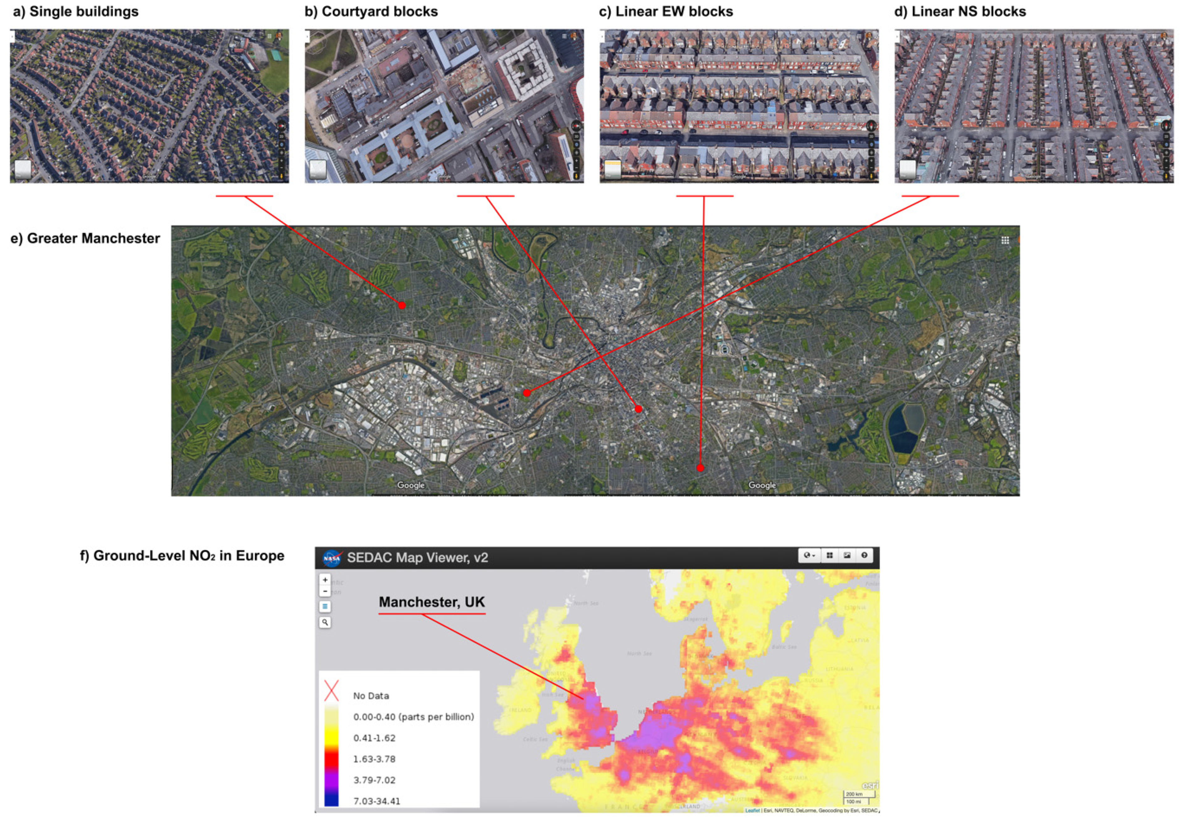
Hence, in this paper, we focus on the dispersion effect of urban forms. Cities are designed (and/or evolved) with different forms. Ratti et al. [18] categorised different urban forms to pavilions, slabs, terraces, terrace-courts, pavilion-courts, and courts. These urban forms could be narrowed down to single, linear, and courtyard forms. In this paper, we will study the impact of these three urban forms on the concentration of air pollution (see Figure 1 for the examples of these urban forms in Manchester, UK). We designed a hypothetical case study with different urban forms. Manchester is one of the most populated cities in the UK, with poor air quality. Annual mortality in Manchester due to air pollution is over a hundred [19]. Among different pollutants, NO2 is one of the main critical ones that harm children, the elderly, and pregnant women. Under some circumstances, NO2 generates secondary pollutants such as ozone (O3), that can lead to further health issues such as asthma among children [20,21]. Therefore, we used hourly measured NO2 data of Manchester to model the impact of different urban forms on the pollution level within a hypothetical neighbourhood. The results of this study can help urban designers and planners, landscape architects, and policymakers to generate pollution-responsive urban design ideas for large cities such as Manchester.
2. Methods
2.1. Air Pollution and Meteorological Data
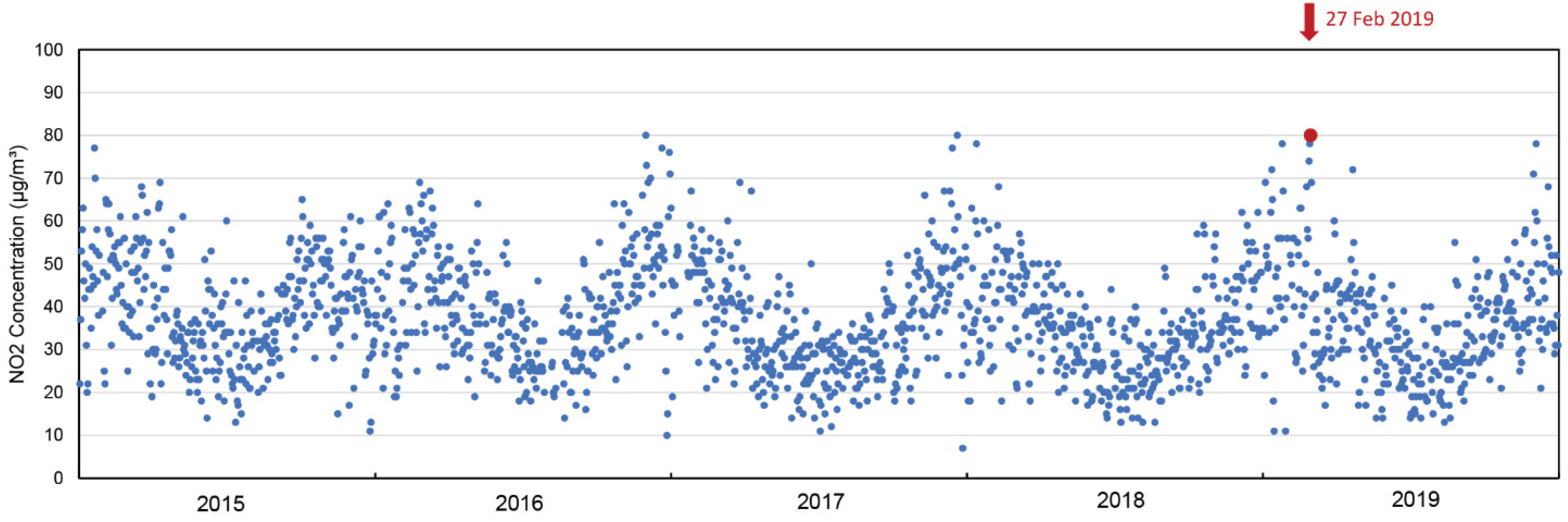
Air pollution (NO2) and meteorological data (air temperatures, wind speed, and relative humidity) in Manchester were retrieved from the UK Department for Environment, Food and Rural Affairs. These data are recorded hourly in the city centre of Manchester (Manchester Piccadilly station). After reviewing the annual data of 2019, we used the data of the most polluted day of the year (27 February 2019). It is worth mentioning that poor air quality in Manchester (and other cities) occurs during the cold periods of the year. This is due to the inversion effect when the height of the urban boundary layer is low [23], and the polluted air does not rise up to by replaced by clean air [24].
Figure 2 shows the daily NO2 concentrations from 2015 to 2019. We highlighted 27 February 2019, which is the day we chose for modelling. On this day, Manchester experienced the highest NO2 concentration in 2019 (80 μg/m3).
2.2. Micrometeorological Models
In this paper, ENVI-met (v 4.3.3 Science) [26] was employed to model the dispersion of air pollution (NO2) within different urban forms. ENVI-met is a CFD model that has four main components to simulate micrometeorological variables. Its components are (a) atmospheric (including turbulence, radiative fluxes, and pollution dispersion), (b) soil model, (c) vegetation, and (d) built environment (the physical domain and urban geometries) [27]. ENVI-met has been used in numerous studies to estimate human thermal comfort, heat mitigation strategies, and urban micrometeorology [28,29].
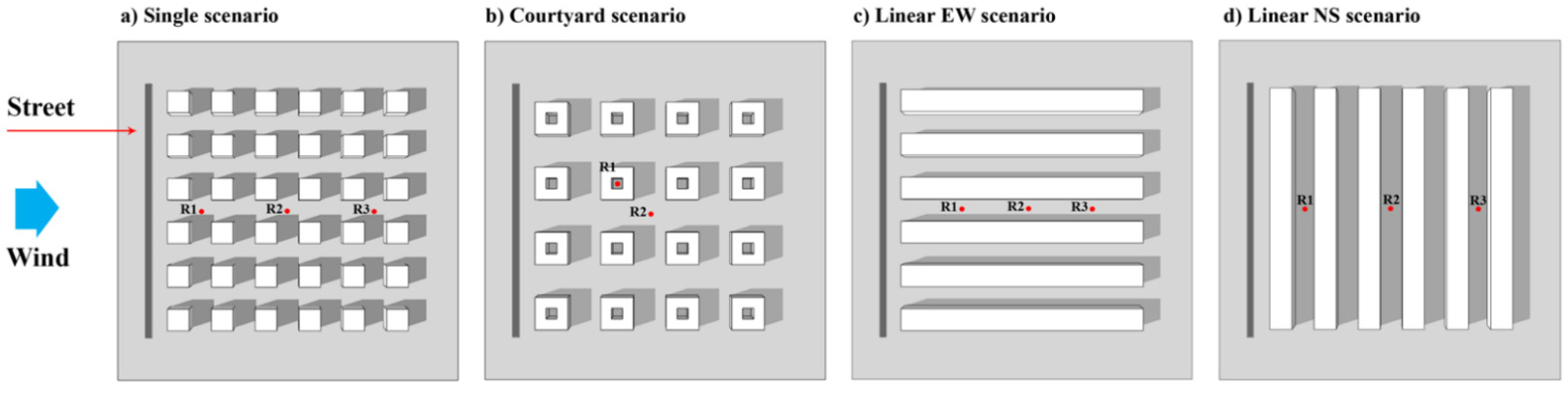
Four scenarios were designed that represent different urban forms (Figure 3). These scenarios are identical in terms of:
- The domain size, which is 160 × 160 × 30 m (x × y × z), and grid cells are 1 × 1 × 1 m (x × y × z).
- The ground surface material is asphalt (albedo 0.1), the building facades are covered with bricks (albedo 0.35), and the roofs are made with tiles (albedo 0.2).
- A street on the left side of the domain that emits pollution (NO2).
The single scenario has identical single urban blocks, which are 10 × 10 × 10 m (x × y × z). The distance between all blocks (urban canyons) is 10 m. The courtyard scenario has courtyard blocks which are 15 × 15 × 10 m (x × y × z). The open space of the courtyard within the blocks is 5 × 5 × 10 m (x × y × z). The urban canyons are 15 m wide. Linear EW and linear NS are similar scenarios with different canyon directions. The length of the long blocks is 110 m, and the width and height are 10 m. The width of the urban canyons is 10 m.
To study the dispersion of pollution, a street line is located on the left side of the domain that emits 80 μg/m3 NO2, at a height of 0.5 m (approximately the height of vehicle exhaust). It should be noted that the only pollutant that we modelled was NO2. A constant wind direction was set from west to east to circulate the street pollution within the scenarios. NO2 and meteorological data to run the simulations were derived from Manchester Piccadilly Gardens station (as mentioned in Section 2.1), and 24 h were simulated, starting from midnight.
ENVI-met employs a standard advection-diffusion equation (Equation (1)) for the dispersion of air pollution [30]:
where A, B, and C are the velocity components of the fluid (air pollution in this case) in x, y, and z directions, respectively.
α is the coefficient of diffusivity which is estimated via Equation (2):
where CT is thermal conductivity, ρ is pressure, and Dρ is the specific heat of the fluid at constant pressure.
α = CT/ρDρ
Manchester is located in the northwest of England. With mild summers (average 20 °C) and cool winters (average 2 °C), the climate is classified as temperate oceanic [31]. Due to global warming, temperatures have reached over 30 °C in summer during recent years. Manchester experiences a high amount of precipitation (810 mm in 2019), much like other British Isles. Different urban forms, such as single urban blocks, courtyard blocks, and linear urban forms, exist in Manchester. Buildings are mostly built by bricks, and streets and sidewalks are paved with asphalt.
3. Results and Discussion
3.1. Validation of the ENVI-Met Model
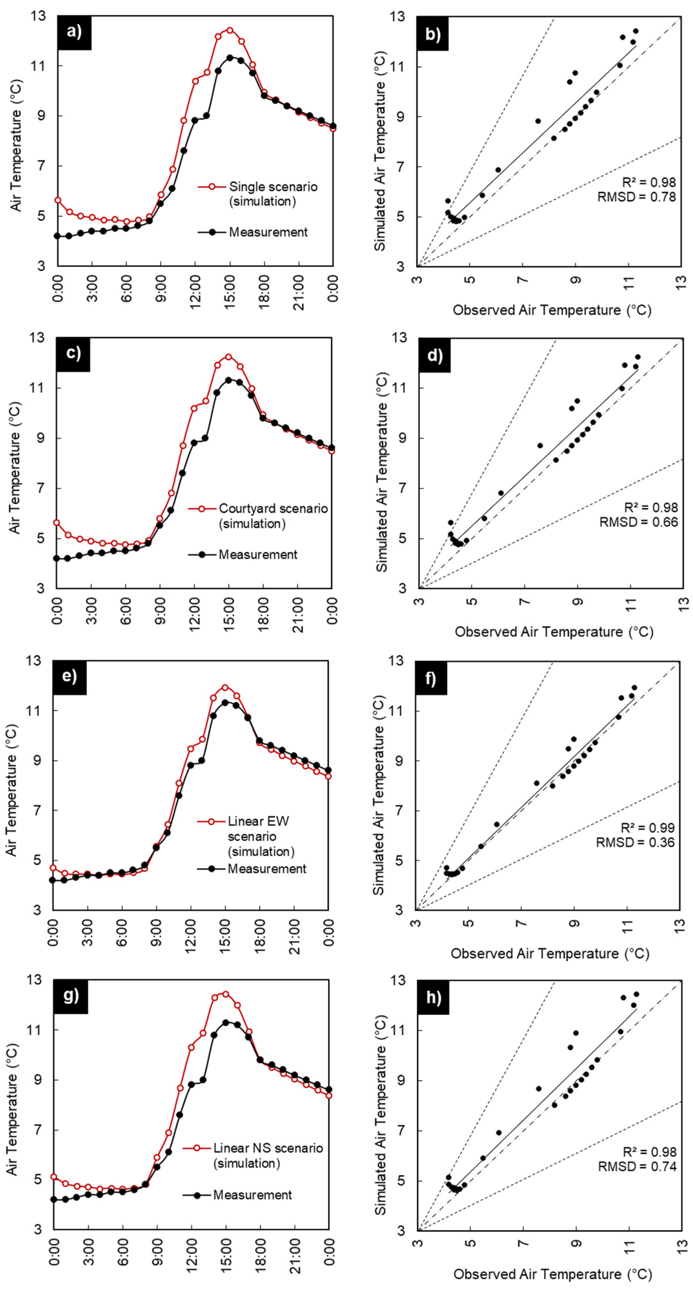
Several studies have validated ENVI-met micrometeorological results, focusing on air temperature [32,33], mean radiant temperature [34,35], surface heat island [36,37], wind speed [38], or thermal comfort [39]. In this study, we compared the measured air temperature from the weather station in Manchester Piccadilly Gardens with the results of ENVI-met in the four scenarios. In the simulated scenarios, we retrieved the air temperature data from the centre of the domains (point R2). Figure 4a,c,e,g show the diurnal comparison of measured versus simulated air temperatures, and Figure 4b,d,f,h show the scatterplots. These panels show the daily average correlation coefficient (R2) and root mean square deviation (RMSD).
In general, the simulated air temperatures show a very close estimation of the measured data. The best results occurred in the linear EW scenario, with an R2 of 99% and RMSD of 0.36 °C. The R2 result indicates that the estimations of ENVI-met from the fluctuations of air temperatures followed 99% similar to the measured data. The RMSD result shows that the accuracy of the ENVI-met estimation is in the range of ±0.36 °C.
In all scenarios, simulated air temperatures overestimated in the early hours, and during 11:00 to 16:00. To sum up, the average daily RMSD in all scenarios was below 0.78 °C.
3.2. Air Pollution in Manchester
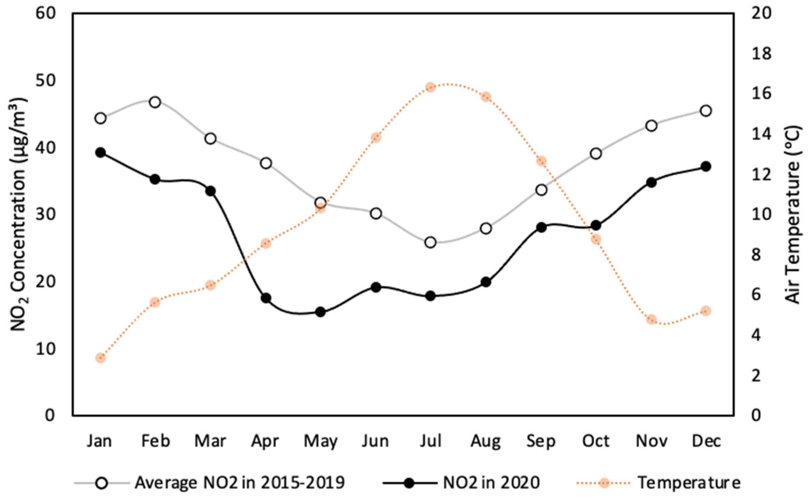
Figure 5 shows the NO2 concentration (on the left vertical axis) and the air temperature (on the right vertical axis). The black and grey curves show NO2 concentrations, and the air temperature data are shown in orange. These data are the average monthly measurements in Manchester (Manchester Piccadilly air pollution station). The monthly NO2 concentrations of 2015–2019 and air temperature datasets show a negative correlation coefficient (−95%). In other words, air pollution is higher in cold months. The maximum monthly NO2 concertation occurred in February (~46.8 μg/m3). In the summertime, minimum pollution occurred in July, with 25.8 μg/m3 when the air temperature was 16.0 °C. The average annual NO2 concentration was 37.3 μg/m3.
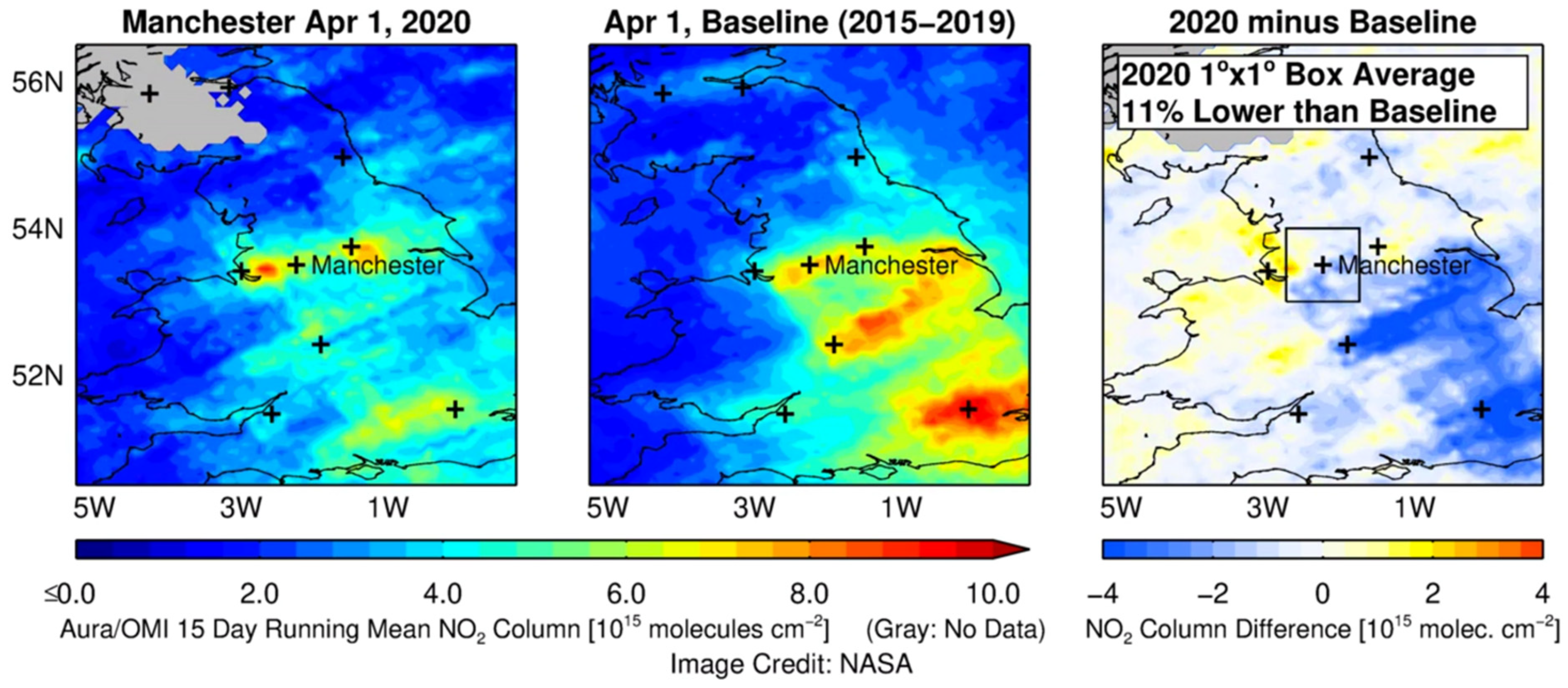
The black line in Figure 5 illustrates the average monthly NO2 concentrations in 2020. The data of this year are shown separately to reflect the impact of the nation-wide lockdown on air pollution in Manchester. The UK government started the working from home policy on 17 March 2020 due to the Coronavirus. This significantly reduced vehicle use. The NO2 concentration in urban environments is highly dependent on vehicle emissions [40,41]. As a result, the NO2 concentration was significantly reduced in 2020. The maximum reductions were seen in April and May, with 20.9 and 17.1 μg/m3 compared to the average data from 2015–2019, respectively. Some businesses opened up in the middle of June in the UK. Appendix A (Figure A1) shows the NO2 concentrations in Manchester on 1 April, compared to a baseline (average 2015–2019). The annual average NO2 in 2015–2019 was 37.3 μg/m3 and in 2020 was 27.2 μg/m3.
3.3. Comparison of Air Pollution within the Four Scenarios
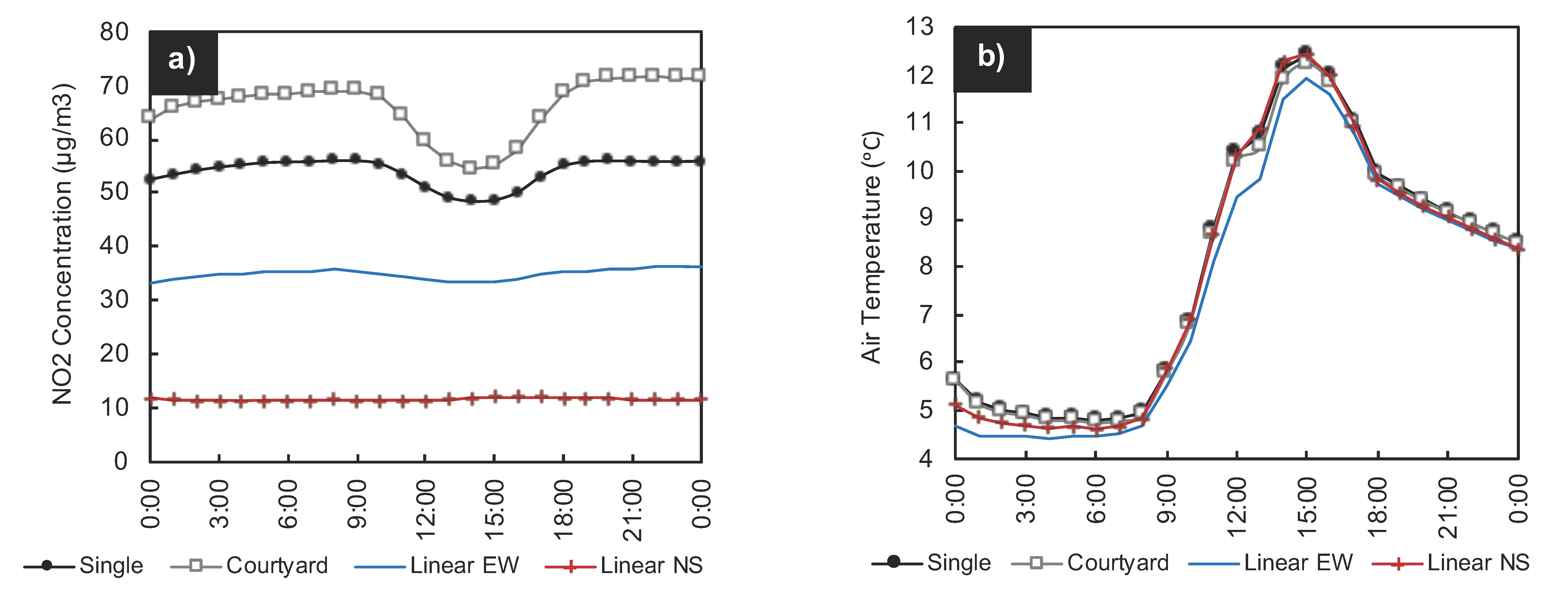
It was discussed that the air pollution (NO2) level has a direct (and negative) correlation with air temperature. Here, we compared NO2 concentrations and air temperatures in different simulation scenarios that were shown in Figure 3. Figure 6 shows the diurnal concentrations (panel a) and air temperatures (panel b) in the centre of the simulated domains (receptor point R2 in all scenarios in Figure 3).
Different diurnal NO2 concentrations occurred within the scenarios. The courtyard scenario had the highest average concentration, with 66.2 μg/m3, and linear NS showed the minimum with 11.7 μg/m3. During the warmest hours, single, courtyard, and linear EW scenarios showed a decline in NO2 concentration. This behaviour was seen before in Figure 5.
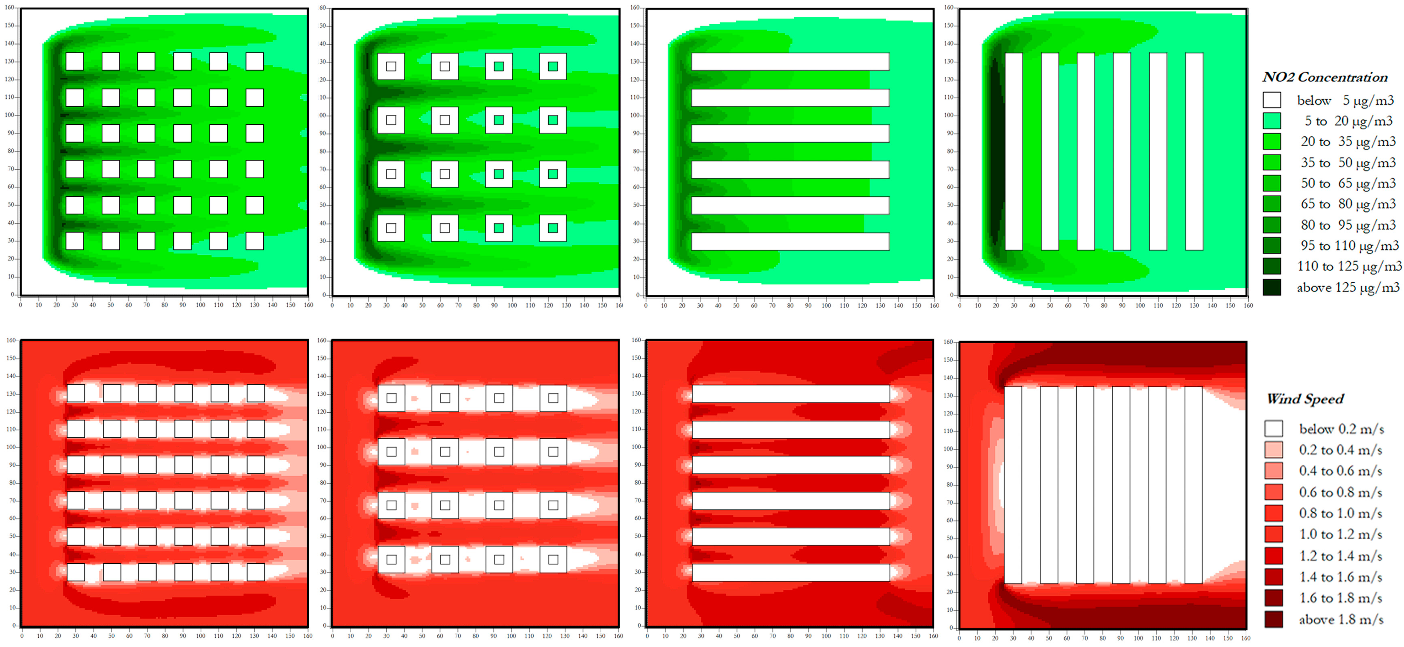
Figure 7 illustrates the distribution of NO2 and wind speed within the scenarios. As the maximum NO2 concentrations occurred at 9 a.m. (see Figure 6a), the panels in Figure 7 show NO2 distribution and wind speed at this time of the day. Among all the scenarios, linear NS traps the pollution close to the street area and keeps the rest of the domain less polluted. This is the reason why the NO2 concentration was significantly lower in linear NS in Figure 6a. This shows that urban geometries and ventilation can significantly change the pollution level. The average wind speed in the centre of the models was 1.0 ms−1 (single), 1.1 ms−1 (courtyard), 1.3 ms−1 (linear EW), and 0.1 ms−1 (linear NS). In summary, Figure 5 showed how temperature variations affect the NO2 concentration, and Figure 7 illustrates how urban forms affect ventilation and consequently the pollution level in a microclimate.
3.4. Spatiotemporal Analysis of the Four Scenarios
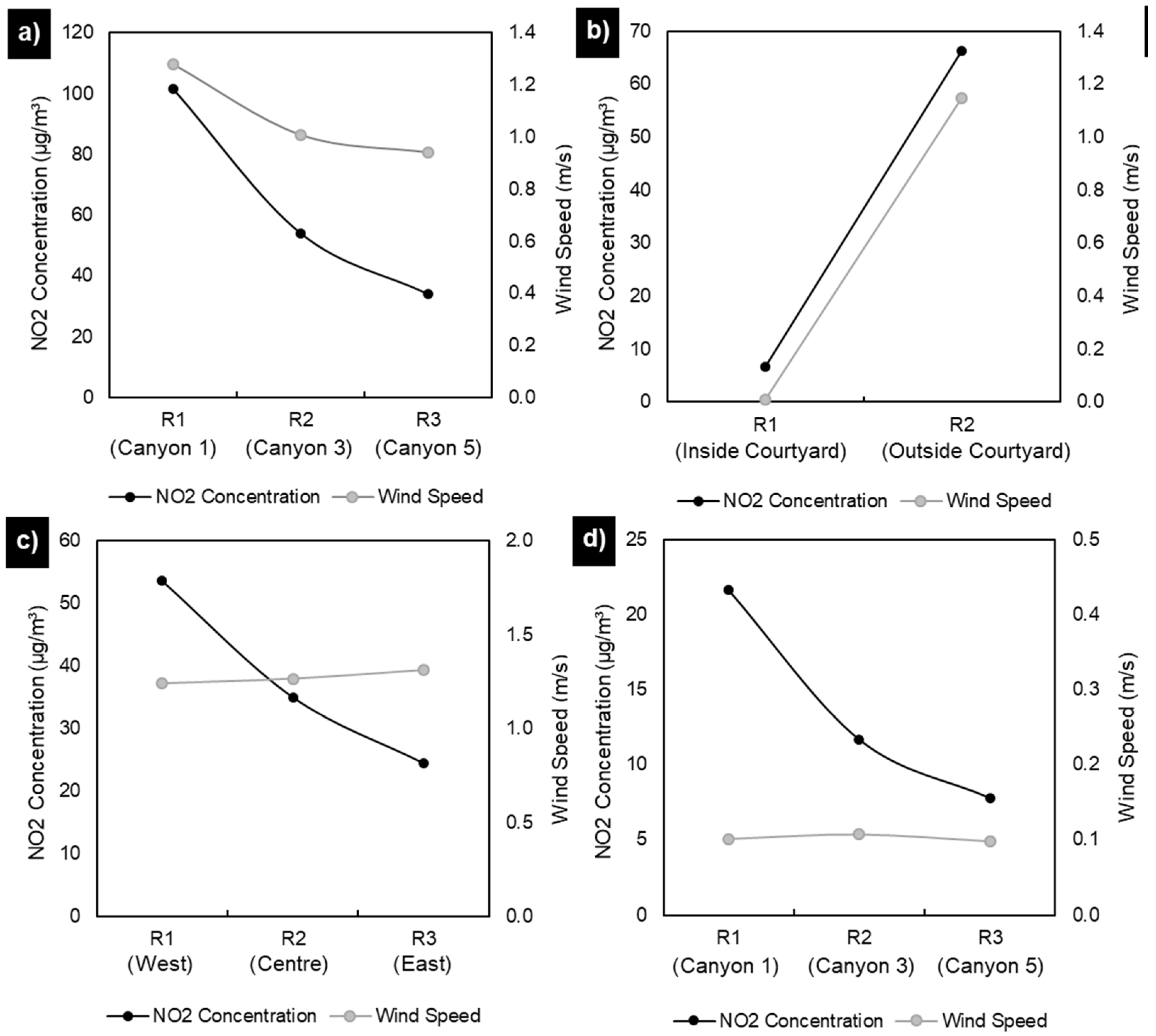
Here, we will individually explore the scenarios. This helps to understand the distribution of pollution in each scenario. In Figure 3a, three receptors were placed in the single scenario. They are in the first (R1), third (R2), and fifth canyons (R3). As Figure 8a shows, the NO2 concentration and wind speed decreased from the first canyon to the fifth one. The correlation coefficient between these two parameters (NO2 concentration and wind) was 95%. The pollution difference between the first canyon (R1) and fifth canyon (R3) was 67 μg/m3 on average during the day. The physical distance between these two points was 80 m.
Regarding the courtyard scenario, R1 is located inside a courtyard, and R2 is placed in the centre of the domain (shown in Figure 3b). Comparing the average NO2 concentration and windspeed shows that the protected environment of the courtyards’ interiors with lower wind speed had a lower NO2 level. The concentration difference between inside and outside of the courtyard was 59 μg/m3 on average during the day.
In the linear EW and linear NS scenarios, the NO2 concentrations also reduced from west to east. At the same time, the wind speed did not significantly change. In linear EW, the concentration difference between the west and east points (R1 and R3) was 30 μg/m3. In the linear NS scenario, the NO2 difference between R1 (first canyon) and R3 (fifth canyon) was 14.2 μg/m3. It is worth mentioning that R3 in the linear EW scenario (24 μg/m3) had a higher NO2 level than R1 in the linear NS scenario (22 μg/m3).
4. Caveats
In this paper, we used the air pollution (NO2) data of Manchester. These data are recorded in the city centre of Manchester (Manchester Piccadilly station), which is one of the busiest areas in the city. It should be noted that this point does not represent the whole city. Therefore, when we analyse the NO2 level in Manchester (Section 3.2), we refer to this area of the city. The other areas in the city with different vegetation fraction, ventilation rate, traffic flow, and other environmental factors may experience lower (or even higher) pollution levels.
Regarding the design of the scenarios, we modelled four hypothetical neighbourhoods that only have one street on their west side. These four urban forms were inspired by the real conditions in the city (Figure 1). We also set a constant wind (for the 24 h) from the west to bring the pollution (NO2) to the neighbourhoods. This allowed us to study the behaviour of the pollution within different neighbourhoods. However, this situation is hardly seen in the real world as:
- (a)
- The emission of air pollution from road traffic is not fixed in a 24 h period. We designed this constant emission to study the impact of air temperature fluctuations on air pollution.
- (b)
- The scenarios only have one street on their west side which emits pollution to the neighbourhoods. The rest of the canyons are considered for pedestrians. In real conditions, it would be hard to find 3 to 5 urban canyons with no polluting vehicles.
- (c)
- This study limited the air pollution to the NO2 that was dispersed from the street. In real life, there are multiple sources of air pollution (such as buildings that use gas for heating or cooling). By excluding such sources, the aim of the paper was to show how different urban forms affect pollution dispersion from a nearby busy road.
Regarding the air pollution that we modelled in this paper, NO2 is not the only pollution type in cities. Different pollutants interact with each other and may generate secondary pollutants under some circumstances. As such, NO2 could lead to ozone (O3) and nitrogen monoxide (NO).
Finally, the results of the NO2 level in each neighbourhood should be limited to the conditions of this study. In other words, although the linear NS scenario reduced NO2 concentrations in this study, other scenarios might perform differently under other circumstances (with different wind directions, or multiple pollutant sources). Therefore, this paper recommends thorough investigation within different urban open spaces based on the prevailing wind direction and the location of pollutant source(s).
5. Conclusions
In the first part of this paper, the air pollution (NO2) level was studied in Manchester, as one of the most polluted cities in the UK. The historic data showed that the NO2 level is higher in winter months. On average, the NO2 concentration in February was 21 μg/m3 higher than in July (45% more), in Manchester. Due to the national lockdown in England, the NO2 concentration was 10.1 μg/m3 lower in 2020 compared to the average of the previous five years (2015–2019). This shows the importance of air pollution reduction in the wintertime, when the vegetation fraction in cities is at its lowest rate in the year.
Proper urban design could be a solution to reduce the negative impacts of air pollution in winter. To study that, four neighbourhoods with different urban forms were designed. The distribution of NO2 in those neighbourhoods was studied on one of the winter days in Manchester with a high pollution level (80 μg/m3 NO2, on the 27 February 2019).
The results showed that the four urban forms responded differently to the identical air pollution source in the neighbourhoods. A fixed wind direction from the west was set up to disperse NO2 from the west side to the rest of the neighbourhoods’ areas. The results showed that the linear NS scenario could block the wind, and consequently NO2 was deviated to the north and south sides of the neighbourhood. This maintained the middle area of the domain as having the lowest amount of NO2. In other scenarios, the NO2 level was higher as the wind was not blocked through the neighbourhoods. It should be noted that as the wind decreased in other scenarios from west to east, the NO2 level was significantly reduced.
The significance of this paper is to show that different urban forms affect the concentration of air pollution for their pedestrians. This finding could be used by urban designers/planners and architects to consider this factor in their early design stages. The urban forms studied in this paper were simplified to make it generalisable. Most significantly, these four urban forms affect the wind pattern, which consequently changes the circulation of the air pollution (NO2 in this case). Therefore, it is important for a designer/planner to consider the prevailing wind direction and the position of air pollution source(s) before designing a neighbourhood. Proper design of a barrier could reduce the air pollution for the population in urban open spaces. In this paper, the experiments showed that the linear NS scenario could block the air pollution coming from the street, and the other urban forms allowed the air pollution to circulate through their neighbourhoods. If changing the urban morphologies was not possible, solid (or green) barriers could be modelled to test their impact(s) on the air quality of an existing neighbourhood.
It should be noted that these urban forms caused different pollution levels based on the location of the polluting street (source) and the constant wind direction from the street. Different sources of pollution and wind directions can develop other situations in urban environments. The experiment conducted in this paper is just one of the possibilities that could occur in the real world. Therefore, this paper suggests thorough modelling of urban air pollution during early design stages.
Funding
This research received no external funding.
Institutional Review Board Statement
Not applicable.
Informed Consent Statement
Not applicable.
Data Availability Statement
Not applicable.
Conflicts of Interest
The authors declare no conflict of interest.
Appendix A

References
- WHO. 7 Million Premature Deaths Annually Linked to Air Pollution. 2014. Available online: http://www.who.int/mediacentre/news/releases/2014/air-pollution/en/ (accessed on 10 October 2017).
- Committee on the Medical Effects of Air Pollutants (COMEAP). The Mortality Effects of Long-Term Exposure to Particulate Air Pollution in the United Kingdom. 2018. Available online: https://assets.publishing.service.gov.uk/government/uploads/system/uploads/attachment_data/file/304641/COMEAP_mortality_effects_of_long_term_exposure.pdf (accessed on 20 March 2019).
- UK-Air. Air Information Resource. 2018. Available online: https://uk-air.defra.gov.uk/ (accessed on 17 September 2018).
- GOV.UK. Plan for Roadside NO2 Concentrations Published. 2017. Available online: https://www.gov.uk/government/news/plan-for-roadside-no2-concentrations-published (accessed on 20 April 2020).
- Directive 2008/50/EC of the European Parliament and of the Council of 21 May 2008 on ambient air quality and cleaner air for Europe. Off. J. Eur. Union 2008, 152, 1–44.
- Nowak, D.J. Quantifying and valuing the role of trees and forests on environmental quality and human health. In Nature and Public Health. Oxford Textbook of Nature and Public Health; van den Bosch, M., Bird, W., Eds.; Oxford University Press: Oxford, UK, 2018; Chapter 10.4; pp. 312–316. [Google Scholar]
- Barwise, Y.; Kumar, P. Designing vegetation barriers for urban air pollution abatement: A practical review for appropriate plant species selection. NPJ Clim. Atmos. Sci. 2020, 3, 12. [Google Scholar] [CrossRef] [Green Version]
- Taleghani, M.; Clark, A.; Swan, W.; Mohegh, A. Air pollution in a microclimate; the impact of different green barriers on the dispersion. Sci. Total Environ. 2020, 711, 134649. [Google Scholar] [CrossRef] [PubMed]
- Abhijith, K.V.; Kumar, P.; Gallagher, J.; McNabola, A.; Baldauf, R.; Pilla, F.; Broderick, B.; Di Sabatino, S.; Pulvirenti, B. Air pollution abatement performances of green infrastructure in open road and built-up street canyon environments—A review. Atmos. Environ. 2017, 162, 71–86. [Google Scholar] [CrossRef]
- Gallagher, J.; Baldauf, R.; Fuller, C.H.; Kumar, P.; Gill, L.W.; McNabola, A. Passive methods for improving air quality in the built environment: A review of porous and solid barriers. Atmos. Environ. 2015, 120, 61–70. [Google Scholar] [CrossRef]
- Abhijith, K.V.; Kumar, P. Field investigations for evaluating green infrastructure effects on air quality in open-road conditions. Atmos. Environ. 2019, 201, 132–147. [Google Scholar] [CrossRef]
- Shaw, C.; Boulic, M.; Longley, I.; Mitchell, T.; Pierse, N.; Howden-Chapman, P. The association between indoor and outdoor NO2 levels: A case study in 50 residences in an urban neighbourhood in New Zealand. Sustain. Cities Soc. 2020, 56, 102093. [Google Scholar] [CrossRef]
- Shrestha, P.M.; Humphrey, J.L.; Carlton, E.J.; Adgate, J.L.; Barton, K.E.; Root, E.D.; Miller, S.L. Impact of Outdoor Air Pollution on Indoor Air Quality in Low-Income Homes during Wildfire Seasons. Int. J. Environ. Res. Public Health 2019, 16, 3535. [Google Scholar] [CrossRef] [Green Version]
- Liu, Y.; Wu, J.; Yu, D.; Ma, Q. The relationship between urban form and air pollution depends on seasonality and city size. Environ. Sci. Pollut. Res. 2018, 25, 15554–15567. [Google Scholar] [CrossRef]
- Mansfield, T.J.; Rodriguez, D.A.; Huegy, J.; MacDonald Gibson, J. The Effects of Urban Form on Ambient Air Pollution and Public Health Risk: A Case Study in Raleigh, North Carolina. Risk Anal. 2015, 35, 901–918. [Google Scholar] [CrossRef] [Green Version]
- Abbass, O.A.; Sailor, D.J.; Gall, E.T. Ozone removal efficiency and surface analysis of green and white roof HVAC filters. Build. Environ. 2018, 136, 118–127. [Google Scholar] [CrossRef] [Green Version]
- DEFRA. Impacts of Vegetation on Urban Air Pollution; UK Department for Environment, Food and Rural Affairs: London, UK, 2018.
- Ratti, C.; Raydan, D.; Steemers, K. Building form and environmental performance: Archetypes, analysis and an arid climate. Energy Build. 2003, 35, 49–59. [Google Scholar] [CrossRef]
- Manchester.gov.uk. 2020. Available online: https://secure.manchester.gov.uk/info/200075/pollution/7697/air_quality (accessed on 15 April 2020).
- Achakulwisut, P.; Brauer, M.; Hystad, P.; Anenberg, S.C. Global, national, and urban burdens of paediatric asthma incidence attributable to ambient NO2 pollution: Estimates from global datasets. Lancet Planet. Health 2019, 3, e166–e178. [Google Scholar] [CrossRef] [Green Version]
- Pierangeli, I.; Nieuwenhuijsen, M.J.; Cirach, M.; Rojas-Rueda, D. Health equity and burden of childhood asthma-related to air pollution in Barcelona. Environ. Res. 2020, 186, 109067. [Google Scholar] [CrossRef] [PubMed]
- SEDAC. Socioeconomic Data and Applications Center. 2021. Available online: https://sedac.ciesin.columbia.edu/mapping/viewer/# (accessed on 6 April 2021).
- Oke, T.R. Boundary Layer Climates; Routledge: New York, NY, USA, 1987. [Google Scholar]
- Oke, T.R.; Mills, G.; Christen, A.; Voogt, J.A. Urban Climates; Cambridge University Press: Cambridge, UK, 2017. [Google Scholar]
- UK Air. Data Selector. 2020. Available online: https://uk-air.defra.gov.uk/data/dataselector (accessed on 12 March 2020).
- Bruse, M. ENVI-Met Website. 2020. Available online: http://www.envi-met.com (accessed on 16 April 2020).
- Bruse, M. ENVI-Met 3.0: Updated Model Overview. 2004. Available online: http://www.envi-met.net/documents/papers/overview30.pdf (accessed on 2 October 2018).
- Taleghani, M.; Marshall, A.; Fitton, R.; Swan, W. Renaturing a microclimate: The impact of greening a neighbourhood on indoor thermal comfort during a heatwave in Manchester, UK. Sol Energy. 2019, 182, 245–255. [Google Scholar] [CrossRef]
- Morakinyo, T.E.; Ouyang, W.; Lau, K.K.-L.; Ren, C.; Ng, E. Right tree, right place (urban canyon): Tree species selection approach for optimum urban heat mitigation-development and evaluation. Sci. Total Environ. 2020, 719, 137461. [Google Scholar] [CrossRef] [PubMed]
- Bruse, M. Turbulence Model in ENVI-Met. 2019. Available online: http://www.botworld.info/doku.php?id=kb:turbulence (accessed on 28 May 2019).
- Kottek, M.; Grieser, J.; Beck, C.; Rudolf, B.; Rubel, F. World Map of the Köppen-Geiger climate classification updated. Meteorol. Z. 2006, 15, 259–263. [Google Scholar] [CrossRef]
- López-Cabeza, V.P.; Galan-Marin, C.; Rivera-Gomez, C.; Roa-Fernandez, J. Courtyard microclimate ENVI-met outputs deviation from the experimental data. Build. Environ. 2018, 144, 129–141. [Google Scholar] [CrossRef]
- Hassan Abdallah, A.S.; Hussein, S.W.; Nayel, M. The Impact of outdoor shading strategies on Student thermal comfort in Open Spaces Between Education Building. Sustain. Cities Soc. 2020, 58, 102124. [Google Scholar] [CrossRef]
- Forouzandeh, A. Numerical modeling validation for the microclimate thermal condition of semi-closed courtyard spaces between buildings. Sustain. Cities Soc. 2018, 36, 327–345. [Google Scholar] [CrossRef]
- Gál, C.V.; Kántor, N. Modeling mean radiant temperature in outdoor spaces, A comparative numerical simulation and validation study. Urban Clim. 2020, 32, 100571. [Google Scholar] [CrossRef]
- Taleghani, M.; Swan, W.; Johansson, E.; Ji, Y. Urban cooling: Which façade orientation has the most impact on a microclimate? Sustain. Cities Soc. 2021, 64, 102547. [Google Scholar] [CrossRef]
- Liu, Z.; Cheng, W.; Jim, C.Y.; Morakinyo, T.E.; Shi, Y.; Ng, E. Heat mitigation benefits of urban green and blue infrastructures: A systematic review of modeling techniques, validation and scenario simulation in ENVI-met V4. Build. Environ. 2021, 200, 107939. [Google Scholar] [CrossRef]
- Ayyad, Y.N.; Sharples, S. Envi-MET validation and sensitivity analysis using field measurements in a hot arid climate. In IOP Conference Series: Earth and Environmental Science. 2019: Sustainable Built Environment Conference 2019 Wales: Policy to Practice 24–25 September 2019, Cardiff, Wales; IOP Publishing: Bristol, UK, 2019; Volume 329, p. 012040. [Google Scholar]
- Ibrahim, E.; Ibrahim, Y.; Fahmy, M.; Mahdy, M. Outdoor microclimatic validation for hybrid simulation workflow in hot arid climates against ENVI-met and field measurements. Energy Procedia 2018, 153, 29–34. [Google Scholar]
- Degraeuwe, B.; Thunis, P.; Clappier, A.; Weiss, M.; Lefevbre, W.; Janssen, S.; Vranckx, S. Impact of passenger car Nox emissions and NO2 fractions on urban NO2 pollution–Scenario analysis for the city of Antwerp, Belgium. Atmos. Environ. 2016, 126, 218–224. [Google Scholar] [CrossRef]
- EEA. Explaining Road Transport Emissions; European Environment Agency: Copenhagen, Denmark, 2016. [Google Scholar]
- NASA. Aura/OMI NO2 for Manchester, England. 2020. Available online: https://so2.gsfc.nasa.gov/no2/pix/htmls/Manchester_data.html (accessed on 25 April 2020).
- Krotkov, N.A.; Lamsal, L.N.; Marchenko, S.V.; Bucsela, E.J.; Swartz, W.H.; Joiner, J.; The OMI Core Team. OMI/Aura Nitrogen Dioxide (NO2) Total and Tropospheric Column 1-orbit L2 Swath 13 × 24 km V003; Goddard Earth Sciences Data and Information Services Center (GES DISC): Greenbelt, MD, USA, 2019. [CrossRef]
Figure 1.
(a–e) Different urban forms in Manchester (images are from Google Maps). (f) Ground-level NO2 observed by the Socioeconomic Data and Applications Centre of NASA (SEDAC by Columbia University) [22].
Figure 1.
(a–e) Different urban forms in Manchester (images are from Google Maps). (f) Ground-level NO2 observed by the Socioeconomic Data and Applications Centre of NASA (SEDAC by Columbia University) [22].

Figure 2.
Average daily NO2 concentration in Manchester [25].
Figure 2.
Average daily NO2 concentration in Manchester [25].

Figure 3.
Four modelled scenarios with different urban forms: (a) single, (b) courtyard, (c) linear EW, and (d) linear NS.
Figure 3.
Four modelled scenarios with different urban forms: (a) single, (b) courtyard, (c) linear EW, and (d) linear NS.

Figure 4.
Comparison of measured versus simulated air temperature results in single (a,b), courtyard (c,d), linear EW (e,f), and linear NS (g,h) scenarios.
Figure 4.
Comparison of measured versus simulated air temperature results in single (a,b), courtyard (c,d), linear EW (e,f), and linear NS (g,h) scenarios.

Figure 5.
NO2 concentrations and air temperatures in Manchester.

Figure 6.
Diurnal NO2 concentration (a) and air temperature (b) in the centre of the four scenarios.
Figure 6.
Diurnal NO2 concentration (a) and air temperature (b) in the centre of the four scenarios.

Figure 7.
Spatial distribution of NO2 concentration in the four scenarios at 9 a.m.

Figure 8.
Comparison of wind speed and NO2 concentration within the four scenarios: (a) Single scenario, (b) Courtyard scenario, (c) Linear EW scenario, and (d) Linear NS scenario.
Figure 8.
Comparison of wind speed and NO2 concentration within the four scenarios: (a) Single scenario, (b) Courtyard scenario, (c) Linear EW scenario, and (d) Linear NS scenario.

Publisher’s Note: MDPI stays neutral with regard to jurisdictional claims in published maps and institutional affiliations. |
© 2022 by the author. Licensee MDPI, Basel, Switzerland. This article is an open access article distributed under the terms and conditions of the Creative Commons Attribution (CC BY) license (https://creativecommons.org/licenses/by/4.0/).
Share and Cite
MDPI and ACS Style
Taleghani, M. Air Pollution within Different Urban Forms in Manchester, UK. Climate 2022, 10, 26. https://doi.org/10.3390/cli10020026
AMA Style
Taleghani M. Air Pollution within Different Urban Forms in Manchester, UK. Climate. 2022; 10(2):26. https://doi.org/10.3390/cli10020026
Chicago/Turabian StyleTaleghani, Mohammad. 2022. "Air Pollution within Different Urban Forms in Manchester, UK" Climate 10, no. 2: 26. https://doi.org/10.3390/cli10020026
Note that from the first issue of 2016, this journal uses article numbers instead of page numbers. See further details here.