
Bioaerosols as Evidence of Atmospheric Circulation Anomalies over the Okhotsk Sea and Shantar Islands in the Late Glacial–Holocene

 ,
,  ,
, 

 , and
, and 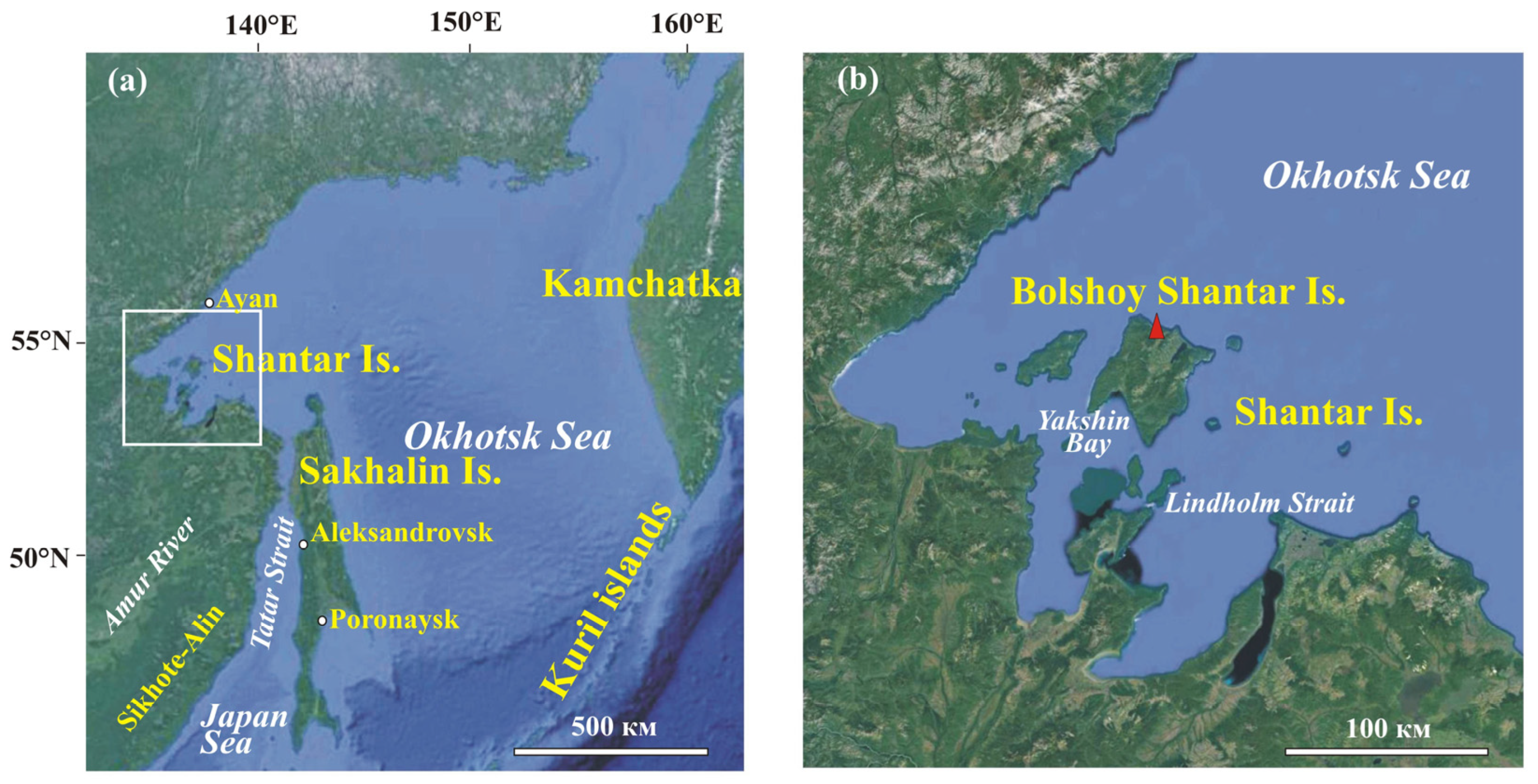
Abstract
:1. Introduction
2. Regional Settings
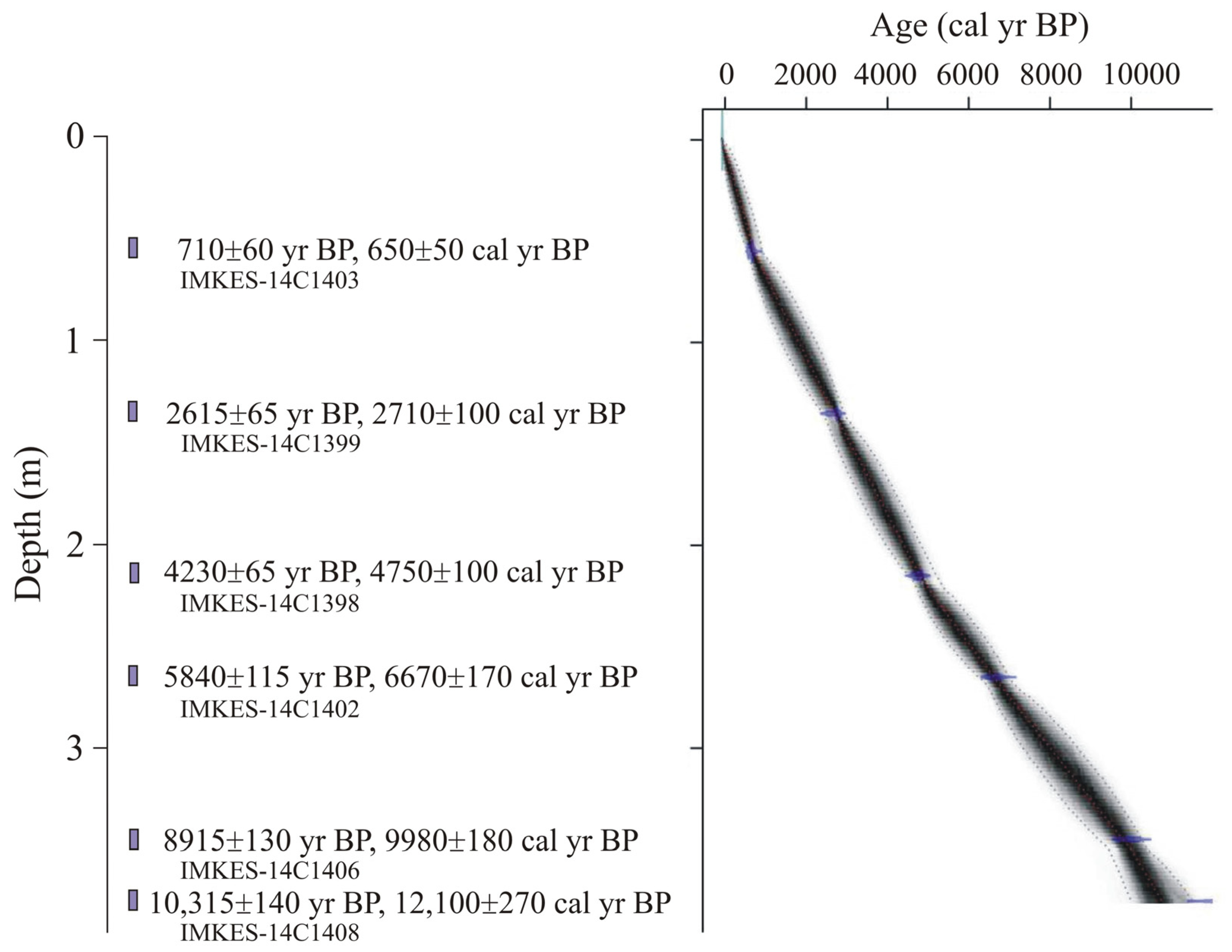
3. Materials and Methods
4. Results
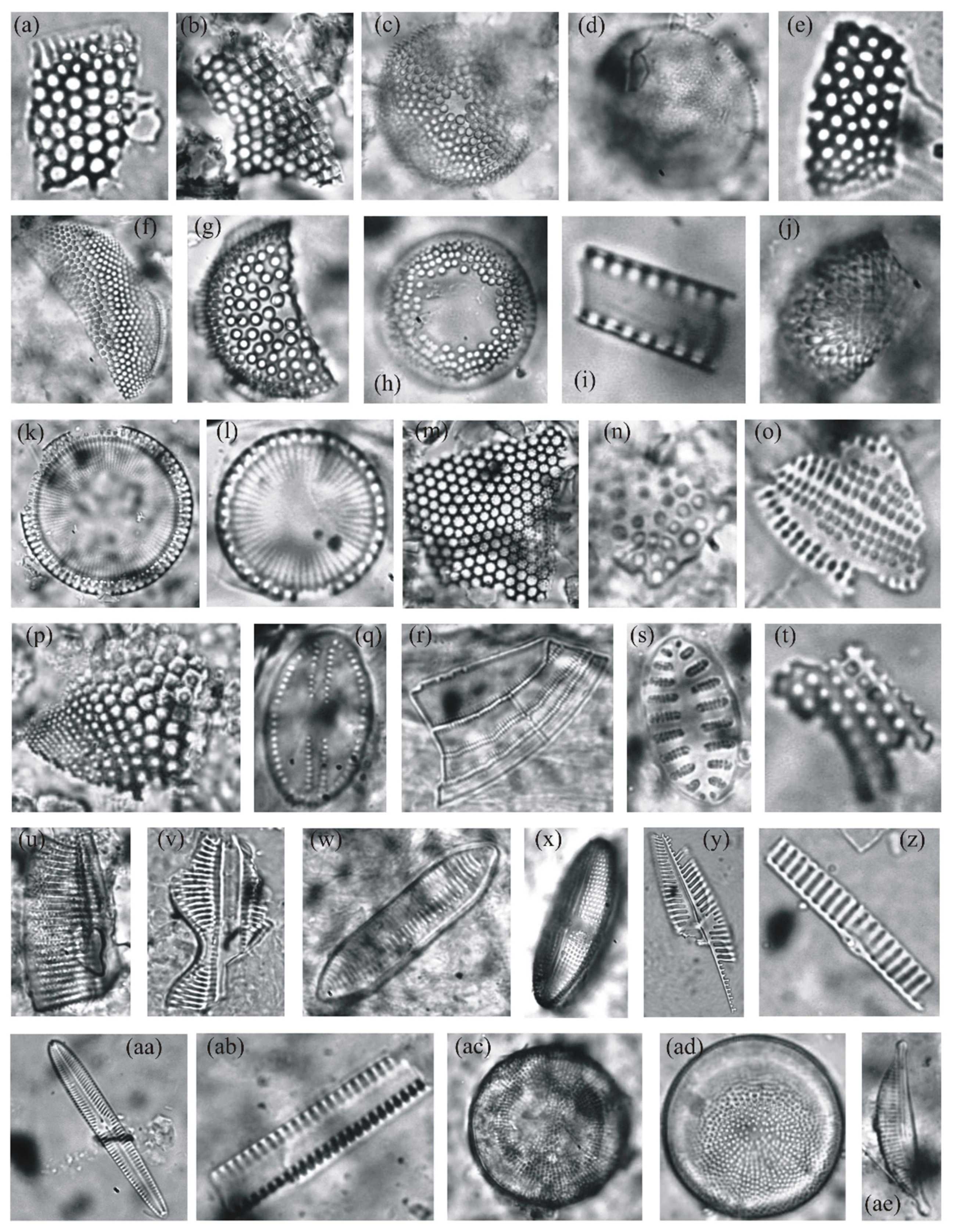
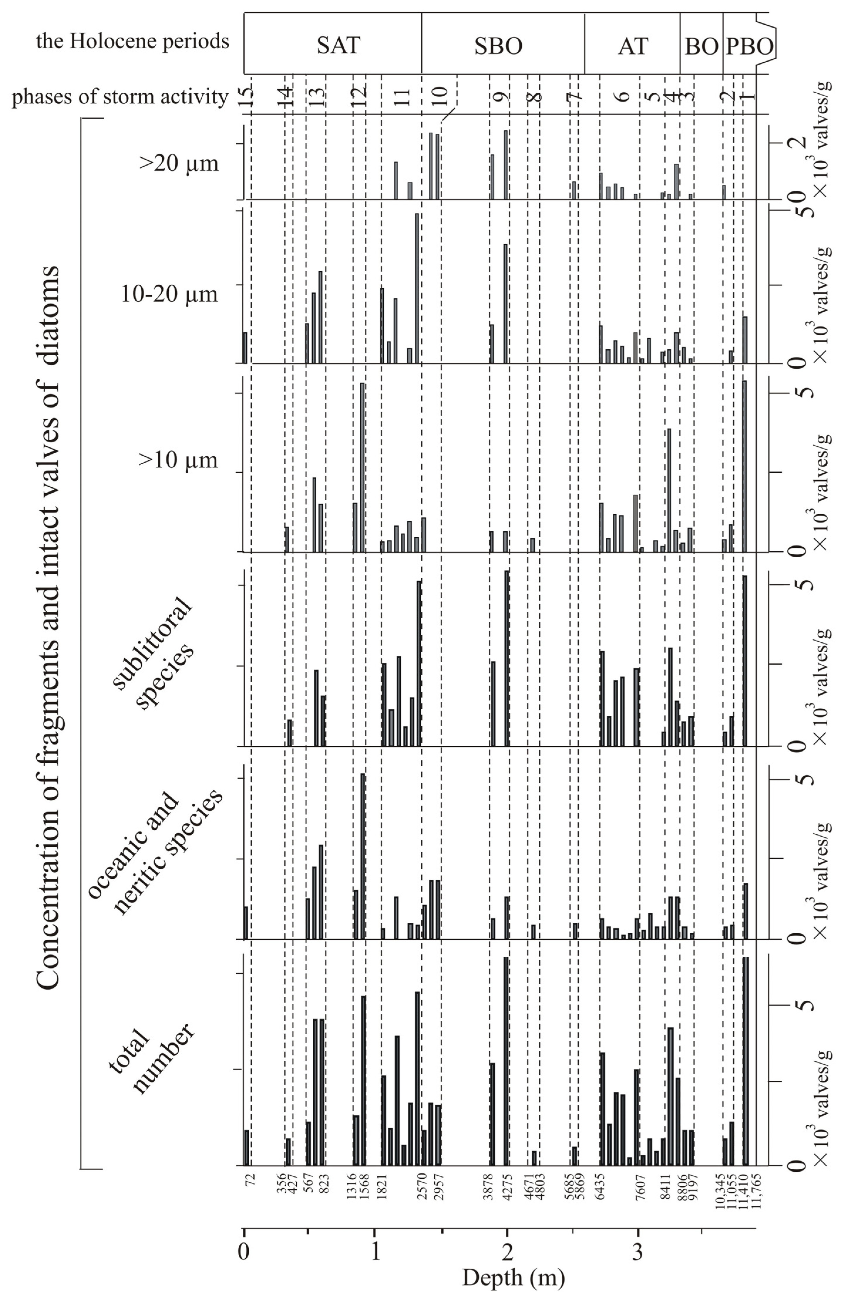
4.1. Diatoms
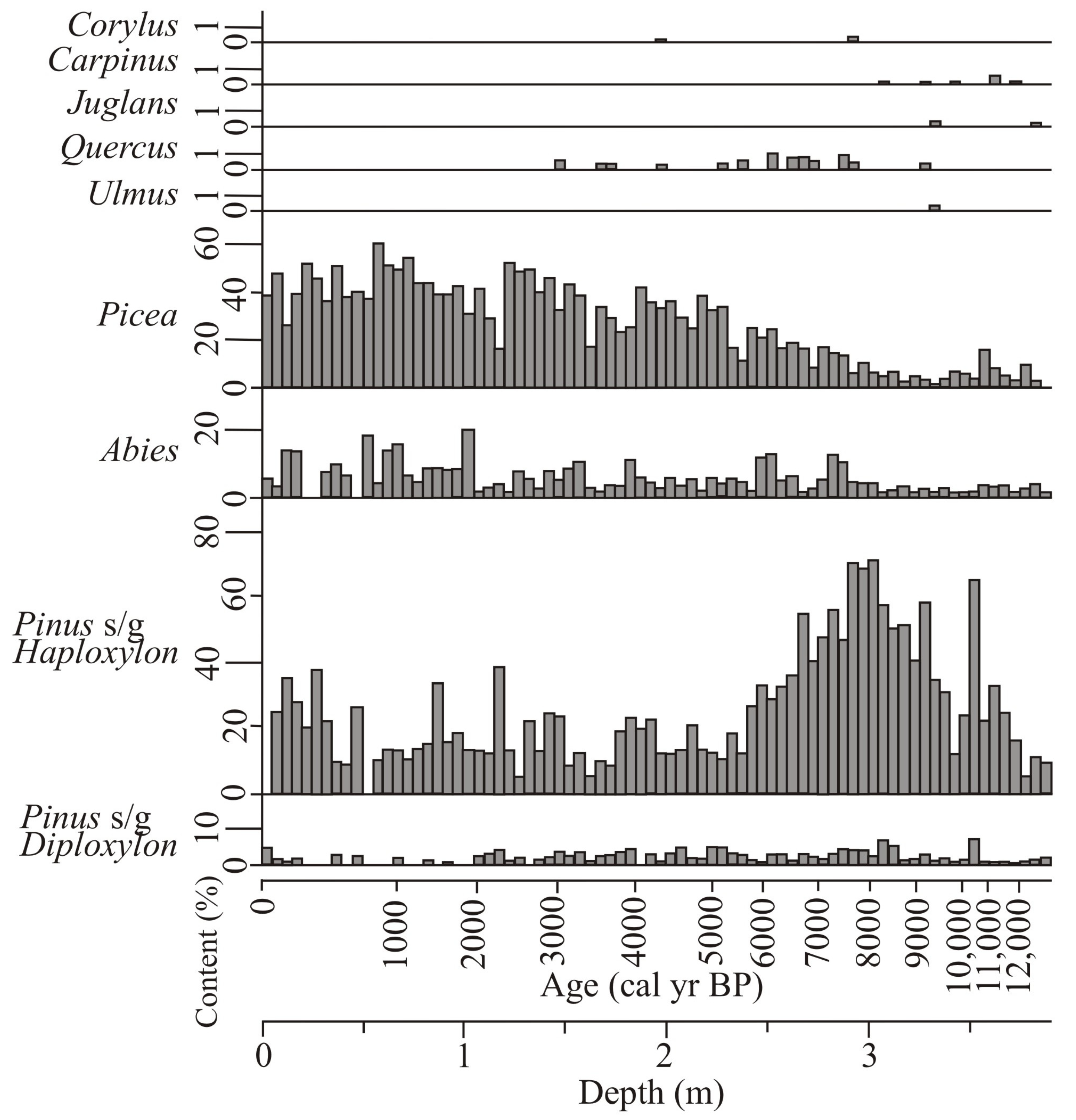
4.2. Pollen
5. Discussion
5.1. Younger Dryas–Early Holocene
5.2. Middle Holocene
5.3. Late Holocene
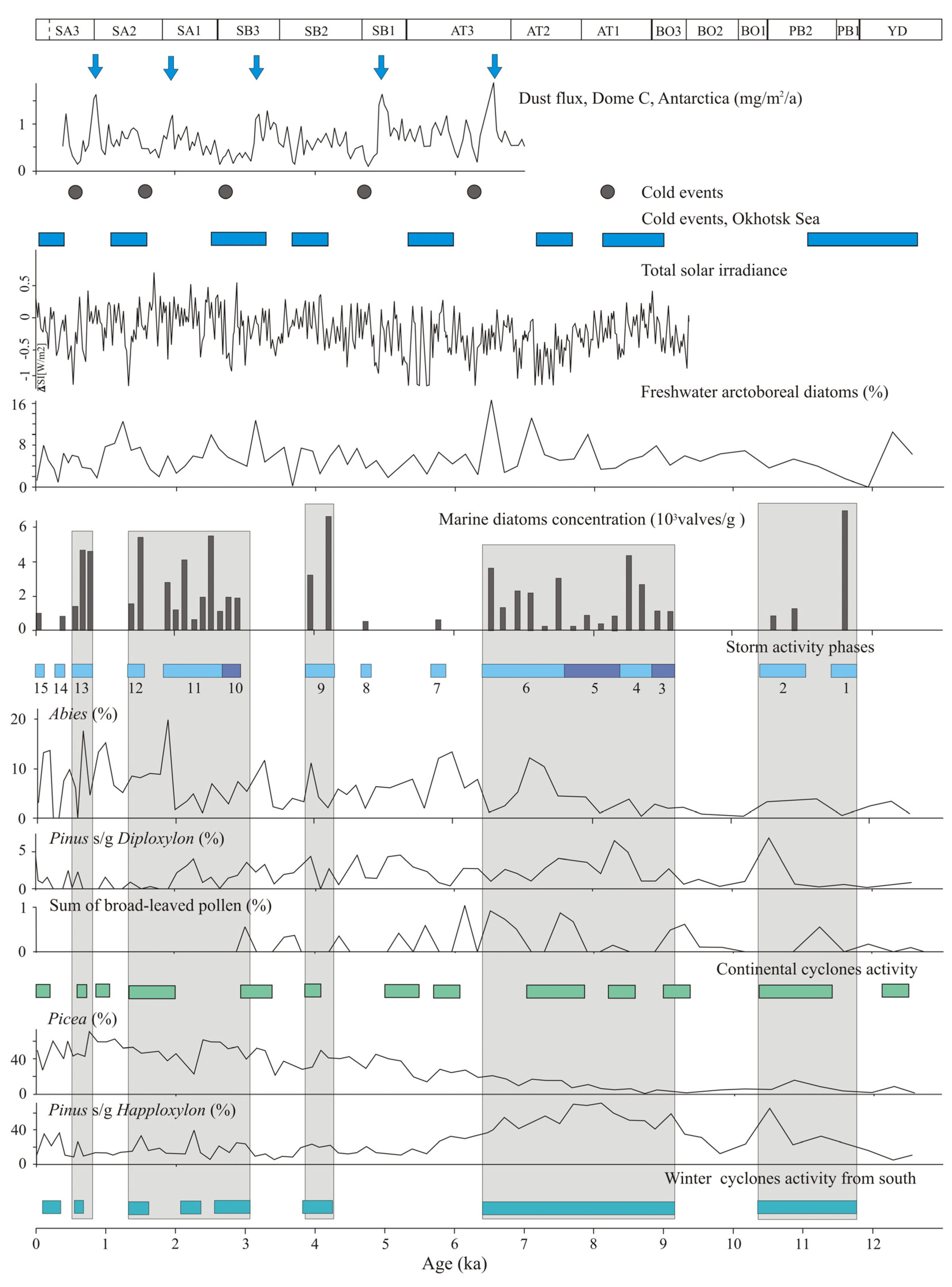
5.4. Typical Changes in Atmosphere Circulation Affecting Bioaerosol Transport
6. Conclusions
Supplementary Materials
Author Contributions
Funding
Institutional Review Board Statement
Informed Consent Statement
Data Availability Statement
Acknowledgments
Conflicts of Interest
References
- Fröhlich-Nowoisky, J.; Kampf, C.J.; Weber, B.; Huffman, J.A.; Pöhlker, C.; Andreae, M.O.; Lang-Yona, N.; Burrows, S.M.; Gunthe, S.S.; Elbert, W.; et al. Bioaerosols in the Earth system: Climate, health, and ecosystem interactions. Atmos. Res. 2016, 182, 346–376. [Google Scholar] [CrossRef] [Green Version]
- Borodulin, A.I.; Safatov, A.S.; Belan, B.D.; Panchenko, M.V. The height distribution and seasonal variations of the tropospheric aerosol biogenic component concentration on the south of western Siberia. J. Aerosol Sci. 2003, 34, 681. [Google Scholar]
- Manninen, H.E.; Back, J.; Sihto-Nissila, S.L.; Huffman, J.A.; Pessi, A.M.; Hiltunen, V.; Aalto, P.P.; Hidalgo, P.J.; Hari, P.; Saarto, A.; et al. Patterns in airborne pollen and other primary biological aerosol particles (PBAP), and their contribution to aerosol mass and number in a boreal forest. Boreal Environ. Res. 2014, 19, 383–405. [Google Scholar]
- Rogers, C.A.; Levetin, E. Evidence of long-distance transport of mountain cedar pollen into Tulsa, Oklahoma. Int. J. Biometerol. 1998, 42, 65–72. [Google Scholar] [CrossRef]
- Misaki, K. Aerosol Behavior. Kise Kenkyu Noto 1981, 142, 95–182. (In Japanese) [Google Scholar]
- Kondrat’ev, I.I. Transboundary Atmospheric Transport of Aerosol and Acid Precipitation to the Russian Far East; Dalnauka: Vladivostok, Russia, 2013. (In Russian) [Google Scholar]
- Hoose, C.; Kristjansson, J.E.; Burrows, S.M. How important is biological ice nucleation in clouds on a global scale? Environ. Res. Lett. 2010, 5, 024009. [Google Scholar] [CrossRef]
- Möhler, O.; DeMott, P.J.; Vali, G.; Levin, Z. Microbiology and atmospheric processes: The role of biological particles in cloud physics. Biogeosciences 2007, 4, 1059–1071. [Google Scholar] [CrossRef] [Green Version]
- Pope, F.D. Pollen grains are efficient cloud condensation nuclei. Environ. Res. Lett. 2010, 5, 044015. [Google Scholar] [CrossRef]
- Steiner, A.L.; Brooks, S.D.; Deng, C.; Thornton, D.C.; Pendleton, M.W.; Bryant, V. Pollen as atmospheric cloud condensation nuclei. Geophys. Res. Lett. 2015, 42, 3596–3602. [Google Scholar] [CrossRef]
- Mikhailov, E.F.; Ivanova, O.A.; Nebosko, E.Y.; Vlasenko, S.S.; Ryshkevich, T.I. Subpollen particles as atmospheric cloud condensation nuclei. Izv. Atmos. Ocean. Phys. 2019, 55, 357–364. [Google Scholar] [CrossRef]
- Taylor, P.E.; Flagan, R.C.; Miguel, A.G.; Valenta, R.; Glovsky, M.M. Birch pollen rupture and the release of aerosols of respirable allergens. Clin. Exp. Allergy 2004, 34, 1591–1596. [Google Scholar] [CrossRef] [PubMed]
- Petrov, E.S.; Novorotskiy, P.V.; Lenshin, V.T. The Climate of the Khabarovsky Krai and the Jewish Autonomous Region; Dalnauka: Khabarovsk, Russia, 2000. (In Russian) [Google Scholar]
- Kimura, N.; Wakatsuchi, M. Increase and decrease of sea ice are in the Sea of Okhotsk: Ice production in coastal polynyas and dynamic thickening in convergence zones. J. Geophys. Res. 2004, 109, C09S03. [Google Scholar] [CrossRef] [Green Version]
- Rogachev, K.A. Satellite observations of regular whirl winds in the bays of the Shantarsky Archipelago, Sea of Okhotsk. Issled. Zemli Iz Kosm. 2012, 1, 54–60. (In Russian) [Google Scholar]
- Rogachev, K.A.; Shlyk, N.V. Jet flow of the Shantarsky Archipelago: Satellite data. Issled. Zemli Iz Kosm. 2014, 5, 68–75. (In Russian) [Google Scholar]
- Terziev, F.S. (Ed.) Hydrometeorology and Hydrochemistry of the Seas. T. IX. Sea of Okhotsk. Issue 1. Hydrometeorological Conditions; Hydrometeoizdat: St. Petersburg, Russia, 1998. (In Russian) [Google Scholar]
- Kulakov, A.P. Quaternary Coastal Lines of Okhotsk and Japan Seas; Nauka: Novosibirsk, Russia, 1973. (In Russian) [Google Scholar]
- Ganeshin, V.G. Origin of the Shantarskie Islands. Priroda 1956, 4, 91–93. (In Russian) [Google Scholar]
- Zhabin, I.A.; Luk’yanova, N.B.; Dubina, V.A. The Water Structure and Dynamics of the Shantar Islands National Park Aquatory (the Sea of Okhotsk) According to Satellite Data. Issled. Zemli Iz Kosm. 2018, 5, 3–14. [Google Scholar] [CrossRef]
- Shlotgauer, S.D.; Kryukova, M.V. Vegetation cover of the Shantarskie Islands. Geogr. Nat. Resour. 2012, 3, 110–114. (In Russian) [Google Scholar]
- Razjigaeva, N.G.; Grebennikova, T.A.; Ganzey, L.A.; Chakov, V.V.; Klimin, M.A.; Mokhova, L.M.; Zakharchenko, E.N. The stratigraphy of the blanket peatland and the development of environments on Bolshoi Shantar Island in the Late Glacial–Holocene. Russ. J. Pac. Geol. 2021, 15, 252–267. [Google Scholar] [CrossRef]
- Blaauw, M.; Christen, J.A. Flexible paleoclimate age-depth models using an 601 autoregressive gamma process. Bayesian Anal. 2011, 6, 457–474. [Google Scholar] [CrossRef]
- Gleser, Z.I.; Jousé, A.P.; Makarova, I.V.; Proshkina-Lavrenko, A.I.; Sheshukova-Poretskaya, V.S. (Eds.) Diatom Algal of the USSR. Fossil and Recent; Nauka: Leningrad, Russia, 1974; Volume 1. (In Russian) [Google Scholar]
- Battarbee, R.W. Diatom analysis. In Handbook of Holocene Paleoecology and Paleohydrology; Berglund, B.E., Ed.; Wiley & Sons: London, UK, 1986; pp. 527–570. [Google Scholar]
- Jouse, A.P. Atlas of Microorganisms in Ocean Bottom Sediments. Diatoms, Radiolarians, Silicoflagellates, Coccoliths; Nauka: Moscow, Russia, 1977. (In Russian) [Google Scholar]
- Loseva, E.I. Atlas of Marine Pleistocene Diatoms of European North-West of USSR; Nauka: St. Peterburg, Russia, 1992. (In Russian) [Google Scholar]
- Tsoy, I.B.; Obrezkova, M.S. Atlas of Diatom Algae and Silicoflagellates from Holocene Sediments of the Russian East Arctic Seas; POI FEB RAS Publ.: Vladivostok, Russia, 2017. (In Russian) [Google Scholar]
- Pokrovskaya, I.M. Methods of paleopollen studies. In Paleopalynology; Pokrovskaya, I.M., Ed.; Nedra: Leningrad, Russia, 1966; pp. 29–60. (In Russian) [Google Scholar]
- Kharkevich, S.S. (Ed.) Vascular Plants of the Soviet Far East; Nauka: Moscow, Russia, 1989; Volume 4. (In Russian) [Google Scholar]
- Takhtajan, A.L. Floristic Areas of the Earth; Nauka: Leningrad, Russia, 1978. (In Russian) [Google Scholar]
- Kharkevich, S.S. (Ed.) Vascular Plants of the Soviet Far East; Nauka: Moscow, Russia, 1991; Volume 5. (In Russian) [Google Scholar]
- Kharkevich, S.S. (Ed.) Vascular Plants of the Soviet Far East; Nauka: Moscow, Russia, 1996; Volume 8. (In Russian) [Google Scholar]
- Kharkevich, S.S. (Ed.) Vascular Plants of the Soviet Far East; Nauka: Moscow, Russia, 1987; Volume 2. (In Russian) [Google Scholar]
- Korotky, A.M.; Pletnev, S.P.; Pushkar, V.S.; Grebennikova, T.A.; Razzhigaeva, N.G.; Sakhebgareeva, E.D.; Mokhova, L.M. Development of Natural Environments of South Far East (the Late Pleistocene-Holocene); Nauka: Moscow, Russia, 1988. (In Russian) [Google Scholar]
- Korotky, A.M.; Grebennikova, T.A.; Pushkar, V.S.; Razzhigaeva, N.G.; Volkov, V.G.; Ganzey, L.A.; Mokhova, L.M.; Bazarova, V.B.; Makarova, T.R. Climatic changes of the territory of South Far East at Late Pleistocene-Holocene. Bull. FEB RAS 1997, 3, 121–143. (In Russian) [Google Scholar]
- Bazarova, V.B. Spreading of broadleaved species in Amur River basin in the Holocene. Bot. Pac. 2014, 3, 47–54. [Google Scholar] [CrossRef] [Green Version]
- Anderson, P.M.; Lozhkin, A.V.; Solomatkina, T.B.; Brown, T.A. Paleoclimatic implications of glacial and postglacial refugia for Pinus pumila in Western Beringia. Quat. Res. 2010, 73, 269–276. [Google Scholar] [CrossRef] [Green Version]
- Hammarlund, D.; Klimaschewski, A.; Amour, N.A.S.; Andrén, E.; Self, A.E.; Solovieva, N.; Andreev, A.A.; Barnekowa, L.; Thomas, W.D.; Edwards, T.W.D. Late Holocene expansion of Siberian dwarf pine (Pinus pumila) in Kamchatka in response to increased snow cover as inferred from lacustrine oxygen-isotope records. Glob. Planet. Change 2015, 134, 91–100. [Google Scholar] [CrossRef]
- Sancetta, C. Oceanographic and ecologic significance of diatoms in surface sediments of the Bering and Okhotsk Seas. Deep-Sea Res. 1981, 28A, 789–817. [Google Scholar] [CrossRef]
- Jouse, A.P. Stratigraphic and Paleogeographic Studies in the Northwest Pacific; Nauka: Moscow, Russia, 1962. (In Russian) [Google Scholar]
- Sancetta, C. Distribution of diatom species in surface sediments of the Bering and Okhotsk seas. Micropaleontology 1982, 28, 221–257. [Google Scholar] [CrossRef]
- Gorbarenko, S.A.; Psheneva OYu Artemova, A.V.; Matul, A.G.; Tiedemann, R.; Nürnberg, D. Paleoenvironment changes in the NW Okhotsk Sea for the last 18 thousand years by micropaleontologic, geochemical, and lithological data. Deep-Sea Res. 2010, 57, 797–811. [Google Scholar] [CrossRef]
- Verkulich, S.R.; Pushina, Z.V.; Dorozhkina, M.V.; Melles, M.; Rethemeyer, J. Characterization of environmental conditions of the interstadial (MIS 3) deposits formation in King George Island (West Antarctica) based on the study of fossil diatom assemblages. Probl. Arct. Antarct. 2015, 3, 109–119. (In Russian) [Google Scholar]
- Nair, A.; Mohan, R.; Shetye, S.; Gazi, S.; Jafar, S.A. Trigonium curvatus sp. nov. and Trigonium arcticum (Bacillariophyceae) from the surface sediments of Prydz Bay, East Antarctica. Micropaleontology 2015, 61, 185–192. [Google Scholar]
- Kharitonov, V.G. Synopsis of Diatom Flora (Bacillariophyceae) of Northern Okhotsk Sea Region; NECSI FEB RAS Publ.: Magadan, Russia, 2010. (In Russian) [Google Scholar]
- Makarova, I.V.; Strelnikova, N.I.; Kozyrenko, T.F.; Gladenkov, A.Y.; Jakovschikova, T.K.; Kazarina, G.K.; Nikolaev, V.A.; Potapova, M.G. (Eds.) The Diatoms of Russia and Adjacent Countries: Fossil and Recent; St.-Petersburg State University Publ.: St. Petersburg, Russia, 2002; Volume II. (In Russian) [Google Scholar]
- Pushkar, V.S.; Cherepanova, M.V.; Likhacheva, O.Y. Detalization of the Pliocene-Quaternary North Pacific diatom zonal scale. Algologia 2014, 24, 94–117. [Google Scholar] [CrossRef] [Green Version]
- Ryabushko, L.I. Diatoms (Bacillariophyta) of the Vostok Bay, Sea of Japan. Biodivers. Environ. Far East Reserves 2014, 2, 4–17. (In Russian) [Google Scholar]
- Tunegolovets, V.P. The intensity of cyclogenesis in the second half of the twentieth century. Izv. TINRO 2009, 151, 140–153. (In Russian) [Google Scholar]
- Sorokin, Y.I. Primary production in the Okhotsk Sea. In Comprehensive Researches of Ecosystem of the Sea of Okhotsk; Sapozhnikov, V.V., Ed.; VNIRO: Moscow, Russia, 1997; pp. 103–110. (In Russian) [Google Scholar]
- Pishchalnik, V.M.; Bobkov, A.O. Oceanographical Atlas of the Sakhalin Shelf; Sakhalin State University: Yuzhno-Sakhalinsk, Russia, 2000. (In Russian) [Google Scholar]
- Yokoyama, Y.; Esat, T.M. Global climate and sea level–enduring variability and rapid fluctuations over the past 150,000 years. Oceanography 2011, 24, 54–67. [Google Scholar] [CrossRef]
- Golovko, V.V.; Koutsenogii, K.P.; Istomin, V.L. Number and mass concentrations of the pollen component of atmospheric aerosol measured near Novosibirsk during blossoming of arboreal plants. Atmos. Ocean. Opt. 2015, 28, 529–533. (In Russian) [Google Scholar] [CrossRef] [Green Version]
- Bazarova, V.B.; Klimin, M.A.; Mokhova, L.M.; Orlova, L.A. New pollen records of Late Pleistocene and Holocene changes of environment and climate in the Lower Amur River basin, NE Eurasia. Quat. Int. 2008, 179, 9–19. [Google Scholar] [CrossRef] [Green Version]
- Razzhigaeva, N.G.; Ganzey, L.A.; Mokhova, L.M.; Grebennikova, T.A.; Panichev, A.M.; Kopoteva, T.A.; Kudryavtseva, E.P.; Arslanov, K.A.; Maksimov, F.E.; Starikova, A.A.; et al. Stages of landscape evolution on the western macroslope of Sikhote-Alin at the Pleistocene–Holocene transition (Bikin River basin). Geogr. Nat. Resour. 2017, 3, 127–138. (In Russian) [Google Scholar]
- Igarashi, Y.; Zharov, E. Climate and vegetation change during the late Pleistocene and early Holocene in Sakhalin and Hokkaido, northeast Asia. Quat. Int. 2011, 237, 24–31. [Google Scholar] [CrossRef]
- Leipe, C.; Nakagawa, T.; Gotanda, K.; Müller, S.; Tarasov, P. Late Quaternary vegetation and climate dynamics at the northern limit of the East Asian summer monsoon and its regional and global-scale controls. Quat. Sci. Rev. 2015, 116, 57–71. [Google Scholar] [CrossRef]
- Razjigaeva, N.G.; Ganzey, L.A.; Grebennikova, T.A.; Mokhova, L.M.; Kopoteva, T.A.; Kudryavtseva, E.P.; Belyanin, P.S.; Panichev, A.M.; Arslanov, K.A.; Maksimov, F.E.; et al. Holocene mountain landscape development and monsoon variation in the southernmost Russian Far East. Boreas 2021, 50, 1043–1058. [Google Scholar] [CrossRef]
- Li, C.; Wu, Y.; Hou, X. Holocene vegetation and climate in Northeast China revealed from Jingbo Lake sediment. Quat. Int. 2011, 229, 67–73. [Google Scholar] [CrossRef]
- Mezentseva, L.I.; Grishina, M.A.; Kondrat’ev, I.I. Trajectories and depth of cyclones entering Primorsky Krai. Bull. FEB RAS 2019, 3, 121–143. (In Russian) [Google Scholar]
- Davis, W.J.; Davis, W.B. Antarctic winds: Pacemaker of global warming, global cooling, and the collapse of civilizations. Climate 2020, 8, 130. [Google Scholar] [CrossRef]
- Steinhilber, F.; Beer, J.; Fröhlich, C. Total solar irradiance during the Holocene. Geophys. Res. Lett. 2009, 36, L19704. [Google Scholar] [CrossRef] [Green Version]
- Wanner, H.; Solomina, O.; Grosjean, M.; Ritz, S.P.; Jetel, M. Structure and origin of Holocene cold events. Quat. Sci. Rev. 2011, 30, 3109–3123. [Google Scholar] [CrossRef]
- Gorbarenko, S.A.; Artemova, A.V.; Goldberg, E.L.; Vasilenko, Y.P. The response of the Okhotsk Sea environment to the orbital-millennium global climate changes during the Last Glacial Maximum, deglaciation and Holocene. Glob. Planet. Change 2014, 116, 76–90. [Google Scholar] [CrossRef]
- Khotinsky, N.A. Holocene of Northern Eurasia; Nauka: Moscow, Russia, 1977. (In Russian) [Google Scholar]
- Katsuki, K.; Khim, B.-K.; Itaki, T. Sea-ice distribution and atmospheric pressure patterns in southwestern Okhotsk Sea since the Last Glacial Maximum. Glob. Planet. Change 2010, 72, 99–107. [Google Scholar] [CrossRef]
- Korotkii, A.M. Quaternary sea-level fluctuations on the Northwestern shelf of the Japan Sea. J. Coast. Res. 1985, 1, 293–298. [Google Scholar]
- Pushkar, V.S.; Cherepanova, M.V. Diatom Assemblages and Correlation of Quaternary Deposits of the Northwestern Pacific Ocean; Dalnauka: Vladivostok, Russia, 2008. (In Russian) [Google Scholar]
- Harada, N.; Katsuki, K.; Nakagawa, M.; Matsumoto, A.; Seki, O.; Addison, J.A.; Finney, B.P.; Sato, M. Holocene sea surface temperature and sea ice extent in the Okhotsk and Bering Seas. Prog. Oceanogr. 2014, 126, 242–253. [Google Scholar] [CrossRef]
- Bazarova, V.B.; Klimin, M.A.; Kopoteva, T.A. Holocene dynamic of Eastern-Asia Monsoon in Lower Amur Area. Geogr. Nat. Resour. 2018, 39, 124–133. [Google Scholar] [CrossRef]
- Chen, R.; Shen, J.; Li, C.; Zhang, E.; Sun, W.; Ji, M. Mid- to late-Holocene East Asian summer monsoon variability recorded in lacustrine sediments from Jingpo Lake, Northeastern China. Holocene 2015, 25, 454–468. [Google Scholar] [CrossRef]
- Kawahata, H.; Ohshima, H.; Shimada, C.; Oba, T. Terrestrial oceanic environmental change in the southern Okhotsk Sea during the Holocene. Quat. Int. 2003, 108, 67–76. [Google Scholar] [CrossRef]
- Mikishin, Y.A.; Gvozdeva, I.G. Early-Middle Holocene of Northern Sakhalin. Bull. NESC FEB RAS 2021, 1, 50–65. [Google Scholar] [CrossRef]
- Razjigaeva, N.G.; Grebennikova, T.A.; Ganzey, L.A.; Ponomarev, V.I.; Gorbunov, A.O.; Klimin, M.A.; Arslanov, K.A.; Maksimov, F.E.; Petrov, A.Y. Recurrence of extreme floods in south Sakhalin Island as evidence of paleo-typhoon variability in North-Western Pacific since 6.6 ka BP. Palaeogeogr. Palaeoclimatol. Palaeoecol. 2020, 556, 109901. [Google Scholar] [CrossRef]
- Korotky, A.M.; Razjigaeva, N.G.; Grebennikova, T.A.; Ganzey, L.A.; Mokhova, L.M.; Bazarova, V.B.; Sulerzhitsky, L.D.; Lutaenko, K.A. Middle and Late Holocene environments and vegetation history of Kunashir Island, Kurile Islands, northwestern Pacific. Holocene 2000, 11, 311–331. [Google Scholar] [CrossRef]
- Itaki, T.; Ikehara, K. Middle to late Holocene changes of the Okhotsk Sea Intermediate Water and their relation to atmospheric circulation. Geophys. Res. Lett. 2004, 31, L24309. [Google Scholar] [CrossRef]
- Denton, G.H.; Karlen, W. Holocene climatic variations. Their pattern and possible cause. Quat. Res. 1973, 3, 155–205. [Google Scholar] [CrossRef]
- Bazarova, V.B.; Grebennikova, T.A.; Orlova, L.A. Natural-environment dynamics within the Amur basin during the neoglacial. Geogr. Nat. Resour. 2014, 35, 275–283. [Google Scholar] [CrossRef]
- Tunegolovets, V.P.; Kochetkova, M.V.; Cherednichenko, U.A. Climatic generalizations of southern cyclones entering the Far Eastern seas and the northwestern part of the Pacific Ocean during the cold season. Izv. TINRO 2009, 151, 109–126. (In Russian) [Google Scholar]
- Glebova, S.Y. Fall-winter cyclogenesis over the Pacific Ocean and Far-Eastern Seas and its influence on development of the sea ice. Izv. TINRO 2017, 191, 147–159. [Google Scholar] [CrossRef] [Green Version]
- Parkinson, C.L. The impact of the Siberian high and Aleutian low on the sea-ice cover of the Sea of Okhotsk. Ann. Glaciol. 1990, 14, 226–229. [Google Scholar] [CrossRef] [Green Version]
- Glebova, S.Y. Cyclones over the Pacific Ocean and Far-Eastern Seas in cold and warm seasons and their influence on wind and thermal regime in the last two decade period. Izv. TINRO 2018, 193, 153–166. [Google Scholar] [CrossRef] [Green Version]
- Martin, S.; Drucker, R.; Yamashita, K. The production of ice and dense shelf water in the Okhotsk Sea polynyas. J. Geophys. Res. 1998, 103, 771–782. [Google Scholar] [CrossRef]
- Il’insky, O.K.; Egorova, M.V. Cyclonic activity over the Okhotsk Sea during cold half year. Tr. FERHRI 1962, 14, 34–38. (In Russian) [Google Scholar]
- Zhang, Y.; Ding, Y.; Li, Q. A climatology of extratropical cyclones over East Asia during 1958–2001. Acta Meteorol. Sin. 2012, 26, 261–277. [Google Scholar] [CrossRef]
- Mesquita, M.D.S.; Hodges, K.I.; Bader, J. Sea-ice anomalies in the Sea of Okhotsk and the relationship with storm tracks in the Northern Hemisphere during winter. Tellus 2011, 63, 312–323. [Google Scholar] [CrossRef] [Green Version]
- Shatilina, T.A.; Tsitsiashvili, G.S.; Radchenkova, T.V. The Okhotsk tropospheric cyclone and its role in the occurrence of extreme air temperature in January in 1950–2019. Izv. TINRO 2021, 201, 64–79. [Google Scholar] [CrossRef]


Publisher’s Note: MDPI stays neutral with regard to jurisdictional claims in published maps and institutional affiliations. |
© 2022 by the authors. Licensee MDPI, Basel, Switzerland. This article is an open access article distributed under the terms and conditions of the Creative Commons Attribution (CC BY) license (https://creativecommons.org/licenses/by/4.0/).
Share and Cite
Razjigaeva, N.; Ganzey, L.; Grebennikova, T.; Ponomarev, V.; Mokhova, L.; Chakov, V.; Klimin, M. Bioaerosols as Evidence of Atmospheric Circulation Anomalies over the Okhotsk Sea and Shantar Islands in the Late Glacial–Holocene. Climate 2022, 10, 24. https://doi.org/10.3390/cli10020024
Razjigaeva N, Ganzey L, Grebennikova T, Ponomarev V, Mokhova L, Chakov V, Klimin M. Bioaerosols as Evidence of Atmospheric Circulation Anomalies over the Okhotsk Sea and Shantar Islands in the Late Glacial–Holocene. Climate. 2022; 10(2):24. https://doi.org/10.3390/cli10020024
Chicago/Turabian StyleRazjigaeva, Nadezhda, Larisa Ganzey, Tatiana Grebennikova, Vladimir Ponomarev, Ludmila Mokhova, Vladimir Chakov, and Mikhail Klimin. 2022. "Bioaerosols as Evidence of Atmospheric Circulation Anomalies over the Okhotsk Sea and Shantar Islands in the Late Glacial–Holocene" Climate 10, no. 2: 24. https://doi.org/10.3390/cli10020024