Article

Suitability Assessment of Weather Networks for Wind Data Measurements in the Athabasca Oil Sands Area

1
Schulich School of Engineering, University of Calgary, Calgary, AB T2N 1N4, Canada
2
Resource Stewardship Division, Alberta Environment and Parks, University Research Park, Calgary, AB T2L 2K8, Canada
*
Author to whom correspondence should be addressed.
Climate 2022, 10(2), 10; https://doi.org/10.3390/cli10020010
Submission received: 2 December 2021 / Revised: 24 December 2021 / Accepted: 15 January 2022 / Published: 18 January 2022
(This article belongs to the Special Issue Climate Change Dynamics and Modeling: Future Perspectives)

Abstract

:
The Athabasca Oil Sands Area (AOSA) in Alberta, Canada, is considered to have a high density of weather stations. Therefore, our objective was to determine an optimal network for the wind data measurement that could sufficiently represent the wind variability in the area. We used available historical data records of the weather stations in the three networks in AOSA, i.e., oil sands monitoring (OSM) water quantity program (WQP) and Wood Buffalo Environmental Association (WBEA) edge sites (ES) and meteorological towers (MT) of the air program. Both graphical and quantitative methods were implemented to find the correlations and similarities in the measurements between weather stations in each network. The graphical method (wind rose diagram) was found as a functional tool to understand the patterns of wind directions, but it was not appropriate to quantify and compare between wind speed data of weather stations. Therefore, we applied the quantitative method of the Pearson correlation coefficient (r) and absolute average error (AAE) in finding a relationship between the wind data of station pairs and the percentage of similarity (PS) method in quantifying the closeness/similarity. In the correlation analyses, we found weak to strong correlations in the wind data of OSM WQP (r = 0.04–0.69) and WBEA ES (r = 0.32–0.77), and a strong correlation (r = 0.33–0.86) in most of the station pairs of the WBEA MT network. In the case of AAE, we did not find any acceptable value within the standard operating procedure (SOP) threshold when logically combining the values of the u and v components together. In the similarity analysis, minor similarities were identified between the stations in the three networks. Hence, we presumed that all weather stations would be required to measure wind data in the AOSA.

1. Introduction

Wind is an important atmospheric element when we think about the current weather condition and predicting the future. It carries temperature and moisture from one place to another, and therefore, weather conditions vary with the shift of wind speed and direction. Both wind speed and wind direction are critical for monitoring and predicting weather patterns and climate from the global to local scale. The wind blows due to uneven heating of the Earth’s surface by the Sun (solar radiation). In this process, the Sun heats the Earth’s surface and warms up the surface air. The warm air becomes less dense and creates a low-pressure zone that tends to rise upwards. Subsequently, denser cold air from the surrounding high-pressure zone blows toward the low-pressure zone due to the pressure gradient, and that causes surface wind [1]. The surface wind recorded at the weather station is directly related to the characteristics of the landscape of the site, i.e., latitude, the roughness of the terrain, surrounding vegetation, and any elevated surface structures [2,3]. Wind observations (i.e., wind speed and direction) have extensive applications in weather monitoring [4] and wind power forecasting [5,6]. For example, studying wind at any place is an initial and critical step to determine the feasibility of intended wind power harnessing through wind farms [3,7]. Moreover, wind is used as a key input parameter for computing the evaporation rate at any place of interest [4]. It also plays a key role in air pollution dispersion [8,9], various agricultural applications like the estimation of crop water requirement and risk assessment of pesticide spray drift [10,11], studying the seasonal variability of rainfall [12,13], and seasonal change predictions [14]. Besides, wind extremes like gusty winds and wind-related disasters, e.g., hurricanes (cyclones) and tornados, could cause immense losses to life and property damages [15,16]. Consequently, the observations of surface wind measurements in weather stations are critical to forecasting such extreme disaster events to plan for the operation and safety at any place in advance [17].
Considering the importance of surface wind measurements, many weather stations record wind speed and direction continuously. For instance, three distinct networks of 17 weather stations are operating in the Athabasca Oil Sands Area (AOSA) for the measurement of meteorological parameters, including surface wind (both speed and direction). These networks are operational under the oil sands monitoring (OSM) water quantity program (WQP) and the Wood Buffalo Environmental Association (WBEA) air program. The WBEA stations are operational as two subnetworks, i.e., edge sites (ES) and meteorological towers (MT). Over 95% of oil sands in Canada reserves are at Alberta (including AOSA, Cold Lake, and Peace River) with a surface area of about 140,000 km2 [18,19], where AOSA alone covers about 66% (a surface area of ~93,259 km2) [20]. Alberta oil sands is known as the fourth-largest volume of proven oil reserves in the world [20]. Therefore, it is a very important region for Alberta Province, and for Canada, that contributes to the local to national economy. Due to the center of the oil sands industry-related activities, it required regular weather monitoring by the three networks to maintain a sustainable environment in AOSA [21,22]. However, one of the questions raised about the density of weather stations in AOSA considering the recommended guidelines of World Meteorological Organization (WMO) for setting up weather stations. In general, the recommended minimum horizontal spacing between two land stations is 250 km in a populated area and 300 km in sparsely populated area [23]. In the case of using the measurements for various weather models, the guidelines recommended at least one station in 10,000, 2500, and 100 km2 areas for the numerical weather prediction model, global model (GM), and regional model (RM), respectively [24]. However, the minimum and maximum distances between stations in each network at AOSA were found approximately 12 and 154 km, 69 and 242 km, and 37 and 186 km for the OSM WQP, WBEA MT, and WBEA ES networks, respectively. Following the WMO recommendation, the weather stations are sufficiently dense in these three networks. Consequently, we opted to investigate the potential of having redundancies of weather stations in measuring the wind speed and direction to be represented for AOSA. The suggested optimization of the networks (from this study) would be, therefore, instrumental in deciding the disposal of redundant stations (if any) and to reduce the financial burden of the operating agencies.
Several methods have been found in the literature for comparing wind data between stations to identify the similarity (i.e., redundancy or closeness). A major stream of literature used each wind component (either, speed, or direction) separately, instead of using them combinedly. For instance, comparisons were performed using only the speed component by linear statistics like the mean or only the direction component by circular statistics like standard deviation, coefficient of variation, skewness, kurtosis, and circular-circular correlation [2,8,25,26,27]. However, it is not appropriate to perform a comparison for a similarity analysis between two datasets (measured at two weather stations) based on the measurements of only a single component (either speed or direction), because wind is a vector quantity that requires to be used combinedly―both the magnitude (speed) and direction together. For example, station A and station B (both at 2-m height) measured wind directions of 5°, and the wind speeds measured by station A and station B were 10 and 20 km/h, respectively. Here, the wind data was 5° with 10 km/h and 5° with 20 km/h for station A and station B, respectively, and they are not similar. Therefore, it would be appropriate to use both components (speed and direction) together as a single entity in a wind data analysis to find similarities. We also observed in the literature that several approaches used both wind components for comparing and performing similarity or closeness between two wind datasets derived from two weather stations [28,29]. These analyses could be grouped into two major categories, such as graphical representation and quantitative measures. The wind rose diagram, a graphical representation, would show a visual to represent the frequency distribution of wind speed and direction over a certain period for any weather station [30]. In contrast, quantitative measures related to the methods included an analysis of association and analysis of coincidence using u (zonal) and v (meridional) for two-dimensional (2D) surface wind vectors of the speed expressed in polar coordinates of the x-direction (east–west) and y-direction (north–south), respectively [28,29,31]. The examples of association-related measures were the Pearson correlation coefficient (r), coefficient of determination (R2), Spearman’s correlation coefficient (RS), Nash–Sutcliffe efficiency (E), and Cosine similarity (Cosθ) [29,32], and the coincidence-related measures were the absolute average error (AAE), relative difference (RD), mean squared error (MSE), root mean square error (RMSE), and bias (B) [1,33,34].
In this study, we considered the approaches that used both u and v components of the surface wind data together as vectors for estimating the similarity or closeness between two datasets of the station pairs in AOSA. The representation of graphical measures, i.e., the wind rose diagram, provided a very good visual in the literature for comparing the datasets between stations; however, it was not possible to derive any quantitative estimates from it. Therefore, we also opted to apply the measure of analysis of association (r, R2, RS, E, and Cosθ) and coincidence (AAE, RD, MSE, RMSE, and B). In the association-related measures, r was widely used in the literature for its capacity of determining the strength and direction of the relationship [32]. AAE was also broadly used among the coincidence-related measures due to providing a more natural measure of the average error and being relatively simple to calculate [35]. These two methods (i.e., r and AAE from the two groups of measure) were found sufficient to measure the quantitative similarity between two datasets to predict one another [36] but did not estimate the number of similar values in each station pair in the datasets. Additionally, we did not find any approach in the literature that considered integrating the error of measuring instrument to quantify the similarity in the wind data. Therefore, we set our overall goal for this study to perform a similarity analysis of historical wind data records of the weather stations in AOSA and identify the minimum number of weather stations required for wind measurements by integrating the instrumental error. The specific objectives to fulfill the overall goal were as follows:
  • Evaluation of graphical and quantitative measures on wind data among weather stations to identify the best representative ones for a similarity analysis;
  • Calculation of the percentage of similarity in the wind data records using the best measures and integrating the instrumental errors to find the correlations among the weather stations; and
  • Determination of optimal weather networks for wind data measurements in the study area based on the estimated percentage of the similarity analysis.

2. Study Area and Data Availability

2.1. Study Area

Our study area was the Athabasca oil sands area, which is in the lower Athabasca River Basin of Northern Alberta, Canada (Figure 1). The Athabasca River drains through the area from southwest towards the north. The landscape varies from upland Boreal forests to poorly drained wetlands within the low land regions [37]. The area is in a subarctic climatic regime with an average annual air temperature from 0.7 to 1 °C and having four seasons of long cold winter, short wet summer, and a short spring and fall. The spring and fall seasons receive a considerable amount of precipitation in terms of snowfall, with an annual total of 376–456 mm. Here, the driest months are from November to April, and the wettest is July. The yearly average wind speed is 9.6 km/h according to the 1961 to 1990 climate normal, where the highest is during spring (10.7 km/h) and the lowest in winter (8.8 km/h) [38]. According to the climate normals from 1981 to 2010, our study area receives an average annual solar radiation of 108–128 W/m2 [39] and records an annual average of the atmospheric pressure 96.9–97.2 kPa, relative humidity 40.1–87.5%, and snow depth up to 30 cm [40].
For monitoring purposes, three networks of weather stations (i.e., OSM WQP, WBEA ES, and WBEA MT) measure the wind speed and direction in the study area, including other meteorological parameters, and span between 109° W and 114° W longitudes and 56° N and 58° N latitudes (Figure 1). Here, the altitudes of the weather stations vary 294–559 m, 299–520 m, and 256–626 m mean sea level for the OSM WQP, WBEA ES, and WBEA MT networks, respectively.

2.2. Data Availability

We collected the available wind speed and wind direction data for 17 stations of the three weather networks from the OSM WQP of Alberta Environment and Parks (AEP) and WBEA for this study. Data measurements of the height, frequency (an averaging window), and period of records of each station are shown in Table 1.

3. Methods

3.1. Graphical Measure

We prepared wind rose diagrams as a graphical visual measure that presents the frequency distribution of both the wind speed and direction data for a period of interest. Here, we synthesized wind rose plots of station pairs in each weather network for each year and compared them side by side to visualize the dynamics in the wind patterns.

3.2. Quantitative Measures

We resolved the wind speed data into scalar quantities (i.e., u and v components were expressed in polar coordinates of the x- and y-directions, respectively) to find the correlation between the measurements of two stations in each station pair in a weather network, as shown in Figure 2. In wind direction measurements, direction refers to the angle from where the wind comes. Here, positive and negative values of the u component considered the wind coming from the west and east, respectively. In the case of the v component, positive and negative values were the south and north. Therefore, first, we transformed the wind direction measurements into the mathematical convention for resolving the scalar wind quantities. Here, we computed the math direction as 270 minus the measured wind direction and added 360 for the negative values. Finally, we computed the relationship between the u and v components for each station data and then compared the stations in each station pair by the correlation measures of the analysis for both association and coincidence (see Section 3.2.1. Association-Related Measures and Section 3.2.2. Coincidence-Related Measures).

3.2.1. Association-Related Measures

We performed a set of association-related measures, such as R2, r, R s , Cosθ, and E, on the entire dataset according to the following equations (Equations (1)–(5)).
R 2 = 1 R S S T S S
r = [ i = 1 n ( D 1 i D 1 ¯ ) ( D 2 i D 2 ¯ ) i = 1 n ( D 1 i   D 1 ¯ ) 2   i = 1 n ( D 2 i D 2 ¯ ) 2 ]
R s = 1 [ 6 i = 1 n D 2 n 3 n ]
C o s θ = i = 1 n D 1 D 2 i = 1 n D 1 2 i = 1 n D 2 2
E = 1 [ i = 1 n ( D 1 D 2 ) 2 i = 1 n ( D 1 D 1 ¯ ) 2 ]
where D1 and D2 are the observational data recorded at Station A and Station B, respectively, the number of observations is n, the residual sum of squares is RSS, and the total sum of squares is TSS.

3.2.2. Coincidence-Related Measures

We embraced several coincidence-related measures, including MSE, AAE, RMSE, B, and RD, and the equations are showing as follows (Equations (6)–(10)). All the symbols used in these equations refer to the meaning of symbols we showed in Section 3.2.1. Association-related measures.
MSE = 1 n   i = 1 n ( D 1 i D 2 i )   2
AAE = 1 n   i = 1 n | ( D 1 i D 2 i ) |
RMSE = 1 n i = 1 n ( D 1 i D 2 i ) 2
B = 1 n   i = 1 n ( D 1 i D 2 i )
RD = 100 n   i = 1 n | D 1 i D 2 i | max ( | D 1 i | , | D 2 i | )

3.2.3. Determination of the Best Representative Measures

We identified a representative measure from each group of the association and coincidence measures to minimize the ambiguity of using several measures. Here, we executed linear regressions among measures in each group to identify the representative measure. In this process, we also identified outliers where the points were significantly away from the best fit regression line [41].

3.3. Similarity Analysis

We conducted a similarity analysis (i.e., percentage of similarity, PS) on the station pairs for the wind data using the acceptable value of instrumental error recommended in the standard operating procedure (SOP) [42,43] using the following equation (Equation (11)):
PS = N 2 N 1   × 100
where N1 refers to the total data count, and N2 is the number of data counts that satisfy the arguments of the absolute difference between D1 and D2, which are ±0.5 m/s (1.8 km/h) for the operational wind speed and ±5° for the wind direction, as suggested in the SOP.

4. Results and Discussion

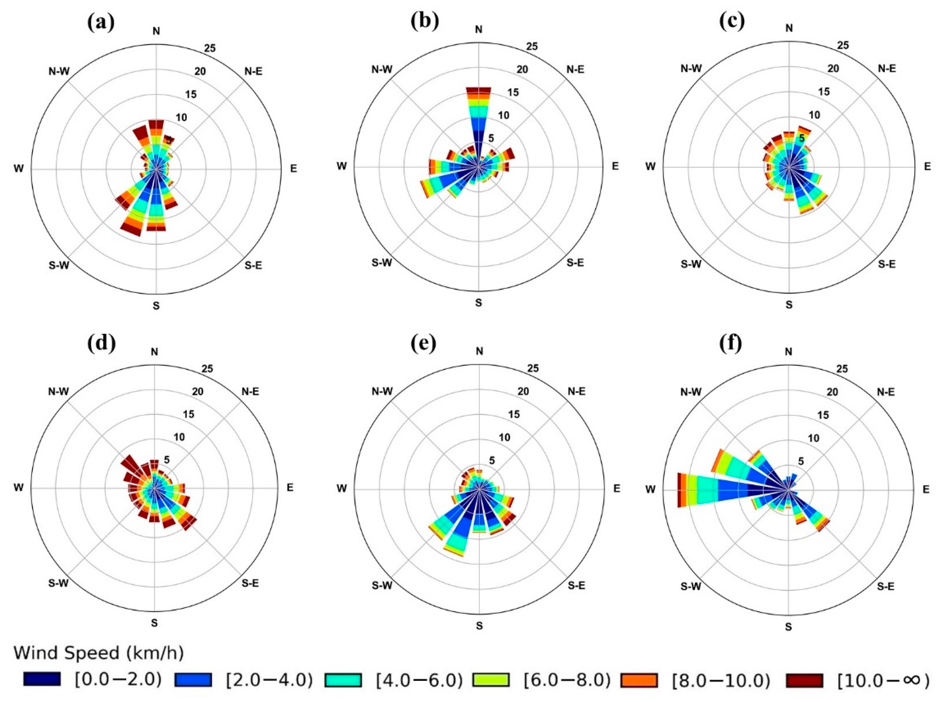
4.1. Wind Rose Diagram

Figure 3 shows wind rose diagrams for OSM WQP stations generated from wind data records measured at the 10-m level for the period 2012–2016. We observed that the dominant wind speed and direction (north: N, south: S, east: E, and west: W) were, respectively, 2–4 km/h and S for C1 (Figure 3a), 6–8 km/h and WSW for C2 (Figure 3b), >10 km/h and SSE for C3 (Figure 3c), 4–6 km/h and SW for C4 (Figure 3d), and 6–8 km/h and S for the C5 (Figure 3e) stations. In the case of the WBEA ES network, the wind rose diagrams were derived from wind data measured at 2-m height for 2015–2017 (see Figure 4). Here, we found the predominant wind speed and direction were, respectively, >10 km/h and SSW for JE306 (Figure 4a), <2 km/h and N for JE308 (Figure 4b), <2 km/h and SE for JE312 (Figure 4c), >10 km/h and SE for JE316 (Figure 4d), <2 km/h and SW for JE323 (Figure 4e), and <2 km/h and W for the R2 (Figure 4f) stations. Wind rose diagrams for WBEA MT stations are presented in Figure 5 and Figure 6.
From the visual comparison of the wind rose diagrams (Figure 3, Figure 4, Figure 5 and Figure 6), we observed significantly different patterns of wind magnitude (speed) and direction among stations. Such variability are likely due to the location of the stations at different altitudes [44] with variations in site characteristics, including the surface roughness and the size, shape, and height of the surrounding vegetations and structures [2,3]. It was straightforward for us to visually identify the dominant wind direction from wind rose diagrams but not for the wind speed. Moreover, we could not quantify the similarity among the wind data measured in the stations from the wind rose diagrams (Figure 3, Figure 4, Figure 5 and Figure 6).

4.2. Measures of Association

Our scatter plot of the association related measures (i.e., R2, RS, Cosθ, and E) against r for the u and v components of the entire wind dataset (see Figure 7a,b) indicated that r could be a representative measure because of its strong association (i.e., R2 > 0.71). Research studies indicated that R2 ≥ 0.50 was significant and acceptable [45,46], and R2 ≥ 0.70 showed a strong association between the two variables [47,48]. Note that we used only positive values of E in this analysis, because values less than zero (i.e., negative values) indicated an unacceptable model performance [49,50]. Therefore, we decided to use r as a representative for the measures of association in finding further similarities between two datasets of station pairs.

4.3. Measures of Coincidence

Our scatter plots of coincidence related measures (i.e., AAE against MSE, RMSE, B, and RD) for the u and v components of the wind datasets (see Figure 8a–d) showed that AAE was strongly correlated with RMSE and MSE (R2 > 0.99). However, we found very low to insignificant relationships of AAE with RD and B. It was because RD is the percentage error (i.e., ratio of absolute difference), while AAE provided only the actual differences [45,46], and the positive and negative differences cancelled each other to provide low values for B [51]. Hence, we considered to use AAE as a representative for the coincidence-related measures in further accomplishing the analysis of similarity between two datasets of station pairs.

4.4. Relationship and Similarity Analysis

We identified that two correlation measures, such as r and AAE (see Section 4.2 and Section 4.3), could represent the best in determining a relationship between two datasets of the wind components for each station pair in the three networks (supported by the results from another study [36]). Here, we considered a strong relationship with r ≥ 0.70 [52,53] and AAE values of ≤1.79 km/h (= 1.8*Cos5°) and ≤0.16 km/h (= 1.8*Sin5°) for the u and v components, respectively. These acceptable AAE values were computed from the acceptable absolute difference values recommended in the SOP, i.e., 1.8 km/h for the wind speed and 5° for the wind direction [42,43]. In addition, we considered at least a 75% value of PS in the similarity analysis to find the closeness of the data values between two stations in a station pair.

4.4.1. Correlation Analysis

OSM WQP network: We observed a very weak to moderate correlation (i.e., r from 0.04 to 0.69) for both the u and v components of all the station pairs, except the station pair C2 vs. C4 for the v component with a strong correlation (r = 0.77) (see Table 2). In addition, we found that AAE values were not acceptable for both the u (2.26–4.14) and v (2.84–5.38) components considering the required acceptable values of ≤1.79 and ≤0.16, respectively. Such a weak-to-moderate correlation and not acceptable AAE values were likely due to factors associated with elevation differences, surface frictions, and the surrounding vegetation of the stations [2,3,44].
WBEA ES network: For both the u and v components, r was satisfied in general (from 0.32 to 0.77) but not the AAE (from 2.05 to 4.33 and 1.57 to 4.26 for the u and v components, respectively). Here, we found two station pairs (i.e., JE306 vs. JE312 and JE312 vs. JE316), where at least one component showed a strong correlation (i.e., r ≥ 0.70), and the other was very close to it (see Table 2). Nevertheless, the reason of not having any acceptable AAE values among the wind datasets would be due to the site-associated factors that cause variable wind magnitude (speed) and direction at any place [54].
WBEA MT network: We found the range of weak to strong correlation values (i.e., r) from 0.35 to 0.82 and 0.33 to 0.86 for the u and v components, respectively (see Table 3). In general, moderate to strong correlations were observed at 16-m and above heights, which would probably be due to the measurements above the vegetation canopy with less interference of the surface roughness [55]. Here, AAE ranged from 0.14 to 0.36, 0.37 to 0.98, 0.63 to 1.43, and 0.93 to 1.83 at 2, 16, 21, and 29-m heights, respectively, for the u component and 0.16 to 0.34, 0.43 to 0.67, 0.63 to 1.16, and 0.91 to 1.88 at 2, 16, 21, and 29-m heights, respectively, for the v component. While all the AAE values of the 15 station pairs were showed as acceptable (i.e., AAE ≤ 1.79) at all heights (except the station pairs of JP107 vs. JP201 with 1.83 and JP201 vs. JP213 with 1.80 at a 29-m height) for the u component, none of those showed the acceptable value (i.e., ≤0.16) at any heights (except the station pair JP104 vs. JP201 with 0.16 at 2-m height) for the v component. However, not a single pair showed acceptable AAE values when we combined both the u and v components together.

4.4.2. Percentage of Similarity

We noticed that the PS values ranged from 8.15 to 16.38%, 3.95 to 30.53%, and 6.94 to 26.16% for the station pairs of the OSM WQP, WBEA ES, and WBEA MT networks, respectively (see Table 4). Note that we considered the SOP values for both the u and v components together in this analysis. Considering such low PS values, we determined that none of the station pairs showed any similarity. Such dissimilarity in wind datasets would likely be due to altitude variations among the weather stations [44]. Landscape or hill forms and its steepness and orientation toward wind would also potentially affect the wind speed and direction [56]. In addition, characteristics of the surrounding vegetation and topographic obstructions in the weather stations would be other factors [2,3]. Moreover, wind direction is difficult to compare even at the same place, because it is highly affected by a lack of synchronization between measurements that allows turbulent motion to make directions quite different [57]. Therefore, it would require wind measurements from all weather stations in the three networks to represent the observed variability in the study area.
Overall, we found variable relationships and similarities in the station pairs of each network, such as: some correlations (i.e., r) in all the networks, no acceptable AAE for the OSM WQP and WBEA ES networks, some acceptable AAE values for the u or v components individually for the WBEA MT network, and no acceptable PS value for any network. Therefore, we did not find any station pair that was acceptable with the logical combination of the “r value” AND “AAE value of the u component” AND “AAE value of the v component” AND “PS value”. We noticed that some stations are spatially very close to each other in the study area, but they belong to other networks. Since we did not find any acceptable station pair in each weather network, we further analyzed for r and AAE (both u and v components) and PS for the closest station pair across the network with the hope of receiving an acceptable correlation and similarity, as an example (see Table 5). For such an analysis, we required the data of station pairs across the network that were measured at the same height, because we should not compare wind data measured at different heights. The closest two station pairs in the cross network were JP104 vs. R2 and JP316 vs. JE316, where all the stations measured data at a 2-m height. The analysis showed a moderate correlation (r = 0.23 and 0.60) with AAE values 1.59 and 4.54 (for the u component) and 2.23 and 3.90 (for the v component) and PS values 6.64 and 4.09% (see Table 5). While reasonable correlations existed in the station pairs, the combination logic of the “r value” AND “AAE value of the u component” AND “AAE value of the v component” AND “PS value” did not show any acceptable station pair suitable from the cross network. It indicated that wind data is more variable at the lower height (e.g., 2 m), where the wind direction might not vary much but the wind speed is greatly impacted by the surrounding landcover, vegetation, topography, and other obstructions and therefore varies much.

5. Conclusions

Weather stations in AOSA were found significantly closer to each other than recommended by the WMO. To understand the redundancy of the stations, we demonstrated that a wind rose diagram would be appropriate for visual comparisons of the wind datasets among weather stations to understand various patterns of the wind magnitude (speed) and direction in the networks. Comparing the dominant wind directions from wind rose diagrams for a station pair was straightforward, but it was difficult for the wind speeds. Therefore, it was not possible to quantify the similarity among the datasets of station pairs from the wind rose diagrams. However, a correlation analysis (i.e., r and AAE) and similarity analysis (i.e., PS) made it possible to quantify the relationship and similarity of the wind data considering the integrated u and v vector components. In the correlation analysis, we observed insignificant correlation in the OSM WQP and WBEA ES networks and a strong correlation in most of the station pairs of the WBEA MT network at 16 m and above heights. However, none of the three networks showed any similarities between the wind data of the station pairs in the similarity analysis. As an example, we performed a similarity analysis between stations across networks for the two closest station pairs but received minor similarities. Note that we did not perform a similarity analysis on the wind data measured across different heights of any station in the WBEA MT network, because the wind speed varies with the level of measurement from the ground. We concluded that all weather stations in the three networks would be required to measure the variability of wind in the study area. Nevertheless, we demonstrated that a similarity analysis would be a decision tool to rationalize/optimize weather stations in a network for wind data measurements. This method of finding similarities would be applicable in optimizing a weather network to minimize the associated costs without sacrificing the scientific credibility of a monitoring program. However, we recommend evaluating these methods thoroughly before applying them to other weather networks in Canada and elsewhere during any decision-making process.

Author Contributions

Conceptualization, D.D., M.R.A., J.A.D., A.G., G.A. and Q.K.H.; Formal analysis, D.D., M.R.A. and J.A.D.; Methodology, D.D., M.R.A., J.A.D., A.G., G.A. and Q.K.H.; Supervision, Q.K.H.; Writing—original draft, D.D. and M.R.A., and Writing—review and editing, J.A.D., A.G., G.A. and Q.K.H. All authors have read and agreed to the published version of the manuscript.

Funding

This research was funded by the Oil Sands Monitoring (OSM) Program of Alberta Environment and Parks (AEP). It was independent of any position of the OSM Program. The fund was awarded to Q.K.H. having an agreement number of 19GRAEM25. OSM had no role in the study design, data collection and analysis, decision to publish, and preparation of the manuscript.

Data Availability Statement

The data used in this study is freely accessible and downloadable from their respective websites. The links are as follows: <http://www.ramp-alberta.org/data/map/default.aspx?c=Climate> (accessed on 1 December 2021) and <https://wbea.org/network-and-data/monitoring-stations/> (accessed on 1 December 2021).

Acknowledgments

The authors of this article would like to acknowledge the Alberta Environment and Parks (AEP) and Wood Buffalo Environmental Association (WBEA) for providing the required data free of cost.

Conflicts of Interest

The authors declare no conflict of interest.

References

  1. Kiranvishnu, K.; Sireesha, K.; Ramprabhakar, J. Comparative Study of Wind Speed Forecasting Techniques. In Proceedings of the 2016 Biennial International Conference on Power and Energy Systems: Towards Sustainable Energy (PESTSE), Bengaluru, India, 21–23 January 2016; pp. 1–6. [Google Scholar] [CrossRef]
  2. Keevallik, S.; Soomere, T.; Pärg, R.; Žukova, V. Outlook for wind measurement at Estonian automatic weather stations. Proc. Est. Acad. Sci. Eng. 2007, 13, 234–251. [Google Scholar]
  3. Ahmed, S.A.; Omer, M.A. Surface wind characteristics and wind direction estimation for “Kalar Region/Sulaimani-North Iraq”. J. Univ. Zakho 2013, 1, 882–890. [Google Scholar]
  4. World Meteorological Organization. Guide to Meteorological Instruments and Methods of Observation, 2010 ed.; WMO-No. 8; World Meteorological Organization (WMO): Geneva, Switzerland, 2010; p. 716. [Google Scholar]
  5. Cassola, F.; Burlando, M. Wind speed and wind energy forecast through Kalman filtering of Numerical Weather Prediction model output. Appl. Energy 2012, 99, 154–166. [Google Scholar] [CrossRef]
  6. Liu, H.; Chen, C. Data processing strategies in wind energy forecasting models and applications: A comprehensive review. Appl. Energy 2019, 249, 392–408. [Google Scholar] [CrossRef]
  7. Rehman, S.; El-Amin, I.M.; Ahmad, F.; Shaahid, S.M.; Al-Shehri, A.M.; Bakhashwain, J.M. Wind power resource assessment for Rafha, Saudi Arabia. Renew. Sustain. Energy Rev. 2007, 11, 937–950. [Google Scholar] [CrossRef]
  8. Belu, R.; Koracin, D. Statistical and spectral analysis of wind characteristics relevant to wind energy assessment using tower measurements in complex terrain. J. Wind Energy 2013, 2013, 1–12. [Google Scholar] [CrossRef]
  9. Carlotti, P. Urban fluid mechanics: Current issues and trends—Summary of the special symposium on urban fluid mechanics at the ASME 2014 4th joint US-European fluid engineering division summer meeting. Environ. Fluid Mech. 2015, 15, 483–490. [Google Scholar] [CrossRef]
  10. Allen, B.R.G.; Wright, J.L. Translating wind measurements from weather stations to agricultural crops. J. Hydrol. Eng. 1997, 2, 26–35. [Google Scholar] [CrossRef] [Green Version]
  11. Desmarteau, D.A.; Ritter, A.M.; Hendley, P.; Guevara, M.W. Impact of wind speed and direction and key meteorological parameters on potential pesticide drift mass loadings from sequential aerial applications. Integr. Environ. Assess. Manag. 2019, 16, 197–210. [Google Scholar] [CrossRef] [PubMed] [Green Version]
  12. Moscati, M.C.D.L.; Gan, M.A. Rainfall variability in the rainy season of semiarid zone of Northeast Brazil (NEB) and its relation to wind regime Marley. Int. J. Climatol. 2007, 27, 493–512. [Google Scholar] [CrossRef]
  13. Hand, L.M.; Shepherd, J.M. An investigation of warm-season spatial rainfall variability in Oklahoma City: Possible linkages to urbanization and prevailing wind. J. Appl. Meteorol. Climatol. 2009, 48, 251–269. [Google Scholar] [CrossRef]
  14. Lledó, L.; Torralba, V.; Soret, A.; Ramon, J.; Doblas-Reyes, F.J. Seasonal forecasts of wind power generation. Renew. Energy 2019, 143, 91–100. [Google Scholar] [CrossRef]
  15. Marchigiani, R.; Gordy, S.; Cipolla, J.; Stawicki, S.A.; Adams, R.C.; Evans, D.C.; Stehly, C.; Galwankar, S.; Russell, S.; Marco, A.P.; et al. Wind disasters: A comprehensive review of current management strategies. Int. J. Crit. Illn. Inj. Sci. 2013, 3, 130–142. [Google Scholar] [CrossRef] [PubMed]
  16. He, Y.; Wu, B.; He, P.; Gu, W.; Liu, B. Wind disasters adaptation in cities in a changing climate: A systematic review. PLoS ONE 2021, 16, e0248503. [Google Scholar] [CrossRef]
  17. Horstmann, J.; Borge, J.C.N.; Seemann, J.; Carrasco, R.; Lund, B. Wind, Wave, and Current Retrieval Utilizing X-Band Marine. In Coastal Ocean Observing Systems; Liu, Y., Kerkering, H., Weisberg, R.H., Eds.; Academic Press: Cambridge, MA, USA, 2015; pp. 281–304. ISBN 9780128020616. [Google Scholar]
  18. Papineau, J.W.; Deacon, L. Fort McMurray and the Canadian Oil Sands: Local Coverage of National Importance. Environ. Commun. 2017, 11, 593–608. [Google Scholar] [CrossRef]
  19. Ahmed, M.R.; Rahaman, K.R.; Hassan, Q.K. Remote sensing of wildland fire-induced risk assessment at the community level. Sensors 2018, 18, 1570. [Google Scholar] [CrossRef] [Green Version]
  20. Oil Sands Community Alliance. The Athabasca Oil Sands Area. Available online: https://www.oscaalberta.ca/did-you-know/the-athabasca-oil-sands-area/ (accessed on 24 November 2021).
  21. Regional Municipality of Wood Buffalo. Envision Wood Buffalo Towards 250k: Fort McMurray—Where We Are Today; Regional Municipality of Wood Buffalo (RMWB): Fort McMurray, AB, Canada, 2008; p. 61. [Google Scholar]
  22. Alberta Envirvonment and Parks. Oil Sands Monitoring Program: Annual Report for 2017–2018; Environment and Climate Change Canada; Government of Alberta: Edmonton, AB, Canada, 2018; p. 64. [Google Scholar]
  23. World Meteorological Organization. Manual on the Global Observing System; WMO-No.544; World Meteorological Organization (WMO): Geneva, Switzerland, 2017; Volume I, p. 172. [Google Scholar]
  24. World Meteorological Organization. Manual on the Global Data-Processing and Forecasting System; WMO-No.485; World Meteorological Organization (WMO): Geneva, Switzerland, 2012; p. 193. [Google Scholar]
  25. Jammalamadaka, S.R.; Seagupta, A. Topics in Circular Statistics (Multivaria Analysis Vol. 5); World Scientific: Singapore, 2001; ISBN 9810237782. [Google Scholar]
  26. Mardia, K.V.; Jupp, P.E. Directional Statistics; John Wiley & Sons, Ltd.: West Sussex, UK, 2000; ISBN 0471953334. [Google Scholar]
  27. Jammalamadaka, S.R.; Lund, U.J. The effect of wind direction on ozone levels: A case study. Environ. Ecol. Stat. 2006, 13, 287–298. [Google Scholar] [CrossRef] [Green Version]
  28. Mohanakumar, K.; Santosh, K.R.; Mohanan, P.; Vasudevan, K.; Manoj, M.G.; Samson, T.K.; Kottayil, A.; Rakesh, V.; Rebello, R.; Abhilash, S. A versatile 205 MHz stratosphere-troposphere radar at Cochin—scientific applications. Curr. Sci. 2018, 114, 2459–2466. [Google Scholar] [CrossRef]
  29. Cohen-Zada, A.L.; Maman, S.; Blumberg, D.G. Earth aeolian wind streaks: Comparison to wind data from model and stations. J. Geophys. Res. Planets 2017, 122, 1119–1137. [Google Scholar] [CrossRef]
  30. Varma, S.A.K.; Srimurali, M.; Varma, S.V.K. Evolution of wind Rose diagrams for RTPP, Kadapa, A.P., India. Int. J. Innov. Res. Dev. 2013, 2, 150–154. [Google Scholar]
  31. Grange, S.K. Technical Note: Averaging Wind Speeds and Directions; University of Auckland: Auckland, New Zealand, 2014; p. 12. [Google Scholar]
  32. Ratner, B. The correlation coefficient: Its values range between 1/1, or do they. J. Target. Meas. Anal. Mark. 2009, 17, 139–142. [Google Scholar] [CrossRef] [Green Version]
  33. Smith, J.; Smith, P. Environmental Modelling. An Introduction; Oxford University Press: Oxford, UK, 2007; ISBN 978019927206. [Google Scholar]
  34. Anderson, J.; Ash, G.; Wright, H. A Statistical Comparison of Weather Stations in Carberry, Manitoba Canada. In 92nd American Meteorological Society Annual Meeting (22–26 January 2012); American Meteorological Society: Boston, MA, USA, 2012; pp. 1–25. [Google Scholar]
  35. Willmott, C.J.; Matsuura, K. Advantages of the mean absolute error (MAE) over the root mean square error (RMSE) in assessing average model performance. Clim. Res. 2005, 30, 79–82. [Google Scholar] [CrossRef]
  36. Deshmukh, D.; Ahmed, M.R.; Dominic, J.A.; Zaghloul, M.S.; Gupta, A.; Achari, G.; Hassan, Q.K. Quantifying relations and similarities of the meteorological parameters among the weather stations in the Alberta Oil Sands region. PLoS ONE 2022, 17, e0261610. [Google Scholar] [CrossRef] [PubMed]
  37. Alberta Environment and Water. Groundwater Flow Model for the Athabasca Oil Sands, North of Fort MacMurray: Phase 1 Conceptual and Numerical Model Development; Environment and Sustainable Resource Development (ESRD): Edmonton, AB, Canada, 2012; p. 325. [Google Scholar]
  38. Suncor Energy Inc. Appendix 3: Climate Change in the Oil Sands Region; Voyageur South Project: Fort McMurray, AB, Canada, 2007; p. 134. [Google Scholar]
  39. Wood Buffalo Environmental Association. WBEA 2000 Annual Report; Wood Buffalo Environmental Association (WBEA): Fort McMurray, AB, Canada, 2000; p. 32. [Google Scholar]
  40. Government of Canada Canadian Climate Normals. Available online: https://climate.weather.gc.ca/climate_normals/index_e.html (accessed on 29 April 2021).
  41. Zou, M.; Djokic, S.Z. A review of approaches for the detection and treatment of outliers in processing wind turbine and wind farm measurements. Energies 2020, 13, 4228. [Google Scholar] [CrossRef]
  42. Government of Alberta Standards and Quality Program. Available online: http://environmentalmonitoring.alberta.ca/resources/standards-and-protocols/ (accessed on 15 December 2020).
  43. World Meteorological Organization. Guide to Instruments and Methods of Observation, 2018 ed.; WMO-No. 8; World Meteorological Organization (WMO): Geneva, Switzerland, 2018; Volume I, p. 573. [Google Scholar]
  44. Turgut, E.T.; Usanmaz, Ö. An analysis of vertical profiles of wind and humidity based on long-term radiosonde data in Turkey. Anadolu Univ. J. Sci. Technol. A—Appl. Sci. Eng. 2016, 17, 830. [Google Scholar]
  45. Mooi, E.; Sarstedt, M. A Concise Guide to Market Research: The Process, Data, and Methods Using IBM SPSS Statistic, 3rd ed.; Springer: Heidelberg, Germany, 2019; ISBN 978-3-662-56706-7. [Google Scholar]
  46. Golmohammadi, G.; Prasher, S.; Madani, A.; Rudra, R. Evaluating three hydrological distributed watershed models: MIKE-SHE, APEX, SWAT. Hydrology 2014, 1, 20–39. [Google Scholar] [CrossRef] [Green Version]
  47. Veiga, V.B.; Hassan, Q.K.; He, J. Development of flow forecasting models in the bow river at Calgary, Alberta, Canada. Water 2015, 7, 99–115. [Google Scholar] [CrossRef] [Green Version]
  48. Anonymous. Coefficient of Determination. Available online: https://www.creativesafetysupply.com/glossary/coefficient-of-determination/ (accessed on 21 April 2021).
  49. Olabanji, M.F.; Ndarana, T.; Davis, N.; Archer, E. Climate change impact on water availability in the olifants catchment (South Africa) with potential adaptation strategies. Phys. Chem. Earth 2020, 120, 102939. [Google Scholar] [CrossRef]
  50. Zhong, X.; Dutta, U. Engaging Nash-Sutcliffe Efficiency and Model Efficiency Factor Indicators in Selecting and Validating Effective Light Rail System Operation and Maintenance Cost Models. J. Traffic Transp. Eng. 2015, 3, 255–265. [Google Scholar] [CrossRef] [Green Version]
  51. Vandeput, N. Forecast KPIs: RMSE, MAE, MAPE & Bias. Available online: https://towardsdatascience.com/forecast-kpi-rmse-mae-mape-bias-cdc5703d242d (accessed on 28 May 2021).
  52. Ramesh, K.; Anitha, R.; Ramalakshmi, P. Prediction of lead seven day minimum and maximum surface air temperature using neural network and genetic programming. Sains Malays. 2015, 44, 1389–1396. [Google Scholar] [CrossRef]
  53. Schober, P.; Schwarte, L.A. Correlation coefficients: Appropriate use and interpretation. Anesth. Analg. 2018, 126, 1763–1768. [Google Scholar] [CrossRef] [PubMed]
  54. Wu, J.; Zha, J.; Zhao, D.; Yang, Q. Changes in terrestrial near-surface wind speed and their possible causes: An overview. Clim. Dyn. 2018, 51, 2039–2078. [Google Scholar] [CrossRef] [Green Version]
  55. Wood Buffalo Environmental Association. WBEA 2019 Annual Report; Wood Buffalo Environmental Association (WBEA): Fort McMurray, AB, Canada, 2020; p. 76. [Google Scholar]
  56. Ruel, J.C.; Pin, D.; Cooper, K. Effect of topography on wind behaviour in a complex terrain. Forestry 1998, 71, 261–265. [Google Scholar] [CrossRef] [Green Version]
  57. Jenkins, G. A comparison between two types of widely used weather stations. Weather 2014, 69, 105–110. [Google Scholar] [CrossRef]
Figure 1. Study area showing the spatial distribution of stations in the weather networks.
Climate 10 00010 g001
Figure 2. Derivation of the x-direction (east-west) and y-direction (north-south) components of the wind data.
Climate 10 00010 g002
Figure 3. Wind rose diagrams for the C1 (a), C2 (b), C3 (c), C4 (d), and C5 (e) stations in the OSM WQP network for the period 2012–2016, where a circular scale is presented as 0–25 in percentage. The latitude and longitude of the stations are: C1 (57.2389° N, 111.4104° W), C2 (57.3833° N, 111.95° W), C3 (57.0273° N, 111.4291° W), C4 (57.5494° N, 111.6533° W), and C5 (56.2236° N, 110.9590° W).
Climate 10 00010 g003
Figure 4. Wind rose diagrams for the JE306 (a), JE308 (b), JE312 (c), JE316 (d), JE323 (e), and R2 (f) stations in the WBEA ES network for the period 2015–2017, where the circular scale is presented as 0–25 in percentage. The latitude and longitude of the stations are: JE306 (57.6218° N, 110.9184° W), JE308 (57.0847° N, 112.8507° W), JE312 (56.8299° N, 110.4345° W), JE316 (56.3528° N, 110.1182° W), JE323 (56.8358° N, 111.1131° W), and R2 (57.1144° N, 111.4289° W).
Climate 10 00010 g004
Figure 5. Wind rose diagrams at 2, 16, 21, and 29-m heights for the JP104 ((ad), respectively); JP107 ((eh), respectively); and JP201 ((il), respectively) stations in the WBEA MT network for the period 2015–2018. Here, the circular scale is presented as 0–25 in percentage. The latitude and longitude of the stations are: JP104 (57.1180° N, 111.4249° W), JP107 (57.8911° N, 111.4348° W), and JP201 (57.0328° N, 113.7345° W).
Climate 10 00010 g005
Figure 6. Wind rose diagrams at 2, 16, 21, and 29-m heights for the JP213 ((ad), respectively); JP311 ((eh), respectively); and JP316 ((il), respectively) stations in the WBEA MT network for the period 2015–2018. Here, the circular scale is presented as 0–25 in percentage. The latitude and longitude of the stations are: JP213 (57.0470° N, 109.7494° W), JP311 (56.5655° N, 111.9485° W), and JP316 (56.3484° N, 110.1213° W).
Climate 10 00010 g006
Figure 7. Measures of association-related relationships among r, R2, and RS (a) and r, Cosθ, and E (b) for the u and v scalar components of the wind dataset. Outliers of E are shown using the solid filled triangles in panel (b).
Climate 10 00010 g007
Figure 8. Relationships of the coincidence-related measures for the entire wind datasets. Here, the relationships are shown for the u component as AAE against RMSE and MSE (a) and RD and B (b) and, for the v component, as AAE against RMSE and MSE (c) and RD and B (d).
Climate 10 00010 g008
Table 1. Availability of wind speed and wind direction data for this study.
NetworkWeather StationData MeasurementPeriod of Records *
Height (m)FrequencyFromTo
OSM WQPC110Daily1 January 200931 March 2017
C222 December 2008
C33 November 2010
C425 July 2011
C51 November 2011
WBEA ESJE3062Hourly3 September 20141 April 2019
JE30825 March 2014
JE3122 September 201431 March 2019
JE3167 March 20141 April 2019
JE32315 March 2014
R21 January 2015
WBEA MTJP1042, 16, 21, and 29Hourly30 May 201431 January 2019
JP10729 August 20121 April 2018
JP20127 May 201431 January 2019
JP21318 July 20121 April 2018
JP31130 July 2013
JP31610 October 2012
* Period of record used in this study.
Table 2. Correlation analysis of the wind components for the OSM WQP and WBEA ES networks.
OSM WQPWBEA ES
Station
Pair
nu-Componentv-ComponentStation
Pair
nu-Componentv-Component
rAAErAAErAAErAAE
C1 vs.C229280.343.260.594.75JE306 vs.JE30820,6280.493.900.582.45
C323380.483.630.692.86JE31237,3320.772.730.691.85
C420760.362.260.542.84JE31637,3800.623.700.633.17
C519750.043.730.484.20JE32318,6730.543.650.632.28
R216,8460.503.760.372.65
C2 vs.C323220.434.140.645.38JE308 vs.JE31220,5760.512.550.662.01
C420600.582.640.773.68JE31623,7520.554.230.612.53
C519750.283.600.534.28JE32322,3840.592.410.671.57
R216,4690.332.640.352.99
C3 vs.C420760.53.810.583.83JE312 vs.JE31637,1660.693.350.772.83
C519750.34.060.535.21JE32318,6910.632.050.721.72
R216,7230.482.570.422.40
C4 vs.C519750.233.180.274.18JE316 vs.JE323
R2
23,0890.714.090.612.58
16,5110.474.330.324.26
JE323 vs.R214,9850.552.070.522.43
Table 3. Correlation analysis of the wind components at different heights in meter (m) for the WBEA MT network.
Station Pair2 m16 m
nu-Componentv-Componentnu-Componentv-Component
rAAErAAErAAErAAE
JP104 vs.JP10731,1210.590.290.330.2832,8350.720.810.590.55
JP20139,9790.430.140.410.1639,9790.530.510.640.46
JP21330,0670.500.340.400.3431,3740.640.610.660.55
JP31129,8550.520.170.480.3432,3940.710.410.600.56
JP31628,3710.500.180.390.1931,2730.660.430.580.45
JP107 vs.JP20131,4860.450.340.490.2633,2300.580.980.520.66
JP21339,9010.730.280.600.2945,0300.760.710.610.60
JP31133,6220.620.310.500.3437,7750.690.890.530.67
JP31633,2270.560.320.500.2742,0240.660.870.550.58
JP201 vs.JP21330,3760.430.360.570.3031,7580.550.680.670.55
JP31130,2110.400.160.680.2732,7920.580.390.780.44
JP31628,4790.350.180.580.1931,5350.470.490.670.49
JP213 vs.JP31134,5850.560.340.620.3237,7010.680.600.690.57
JP31635,5930.590.330.660.2741,6250.730.550.800.43
JP311 vs.JP31630,7320.590.150.630.2935,5520.710.370.780.43
21 m29 m
JP104 vs.JP10732,8420.810.940.560.8632,8340.741.320.641.11
JP20139,9790.501.030.670.8139,9790.431.600.601.27
JP21332,7500.720.960.670.9432,5040.651.370.551.08
JP31132,4020.780.650.681.0232,5400.761.000.481.88
JP31632,1410.720.730.640.8732,1320.691.140.591.50
JP107 vs.JP20133,2390.531.430.511.0933,2310.521.830.501.48
JP21346,8680.771.000.620.9646,6200.771.330.631.38
JP31137,8510.721.140.501.1637,9830.731.360.491.71
JP31642,9010.701.130.610.9142,8680.701.420.621.32
JP201 vs.JP21333,1560.521.260.680.9632,9100.501.800.671.43
JP31132,8040.510.870.770.8532,9420.491.350.761.32
JP31632,3670.450.970.700.8732,3580.441.440.691.35
JP213 vs.JP31139,3910.700.990.700.9739,2770.721.350.691.46
JP31643,7280.800.820.850.6343,4710.821.090.860.91
JP311 vs.JP31636,5080.770.630.780.7736,6370.780.930.771.17
Table 4. Similarity analysis of the wind speed and direction for the three networks.
OSM WQP WBEA ESWBEA MT
Station PairPS (%)Station PairPS (%)Station PairPS (%)
at
10 m
at
2 m
at
2 m
at
16 m
at
21 m
at
29 m
C1 vs. C28.57JE306 vs.JE3087.03JP104 vs.JP10710.2215.1319.1614.51
C316.38JE31214.01JP20113.319.799.789.76
C411.46JE31612.18JP21311.0017.7121.3412.12
C58.76JE3238.63JP3116.949.0012.358.03
R24.93JP3169.6012.9514.6013.50
C2 vs.C38.18JE308 vs.JE31210.72JP107 vs.JP2018.009.4211.0611.00
C413.64JE31619.39JP21320.2220.0521.4020.89
C511.34JE32330.53JP31110.6011.0010.9610.91
R25.67JP31612.7014.4714.6114.38
C3 vs.C48.38JE312 vs.JE31610.05JP201 vs.JP21310.6913.3613.5512.89
C58.15JE32316.94JP31112.9717.2716.1416.38
R29.19JP31610.6015.8215.6914.97
C4 vs.C512.10JE316 vs.JE32318.43JP213 vs.JP31112.4115.0615.7816.98
R23.95JP31615.3923.7424.4126.16
JE323 vs.R29.90JP311 vs.JP31615.7021.2622.7523.96
Table 5. Example of a correlation and similarity analysis across the networks.
Station Pairnu-Componentv-ComponentPS
(%)
rAAErAAE
JP104 vs.R215,7360.231.590.312.236.64
JP316 vs.JE31628,6990.604.540.793.904.09
Publisher’s Note: MDPI stays neutral with regard to jurisdictional claims in published maps and institutional affiliations.

