
Climate Change Impacts on Groundwater Recharge in Cold and Humid Climates: Controlling Processes and Thresholds


Abstract
:
1. Introduction
2. Data and Methods
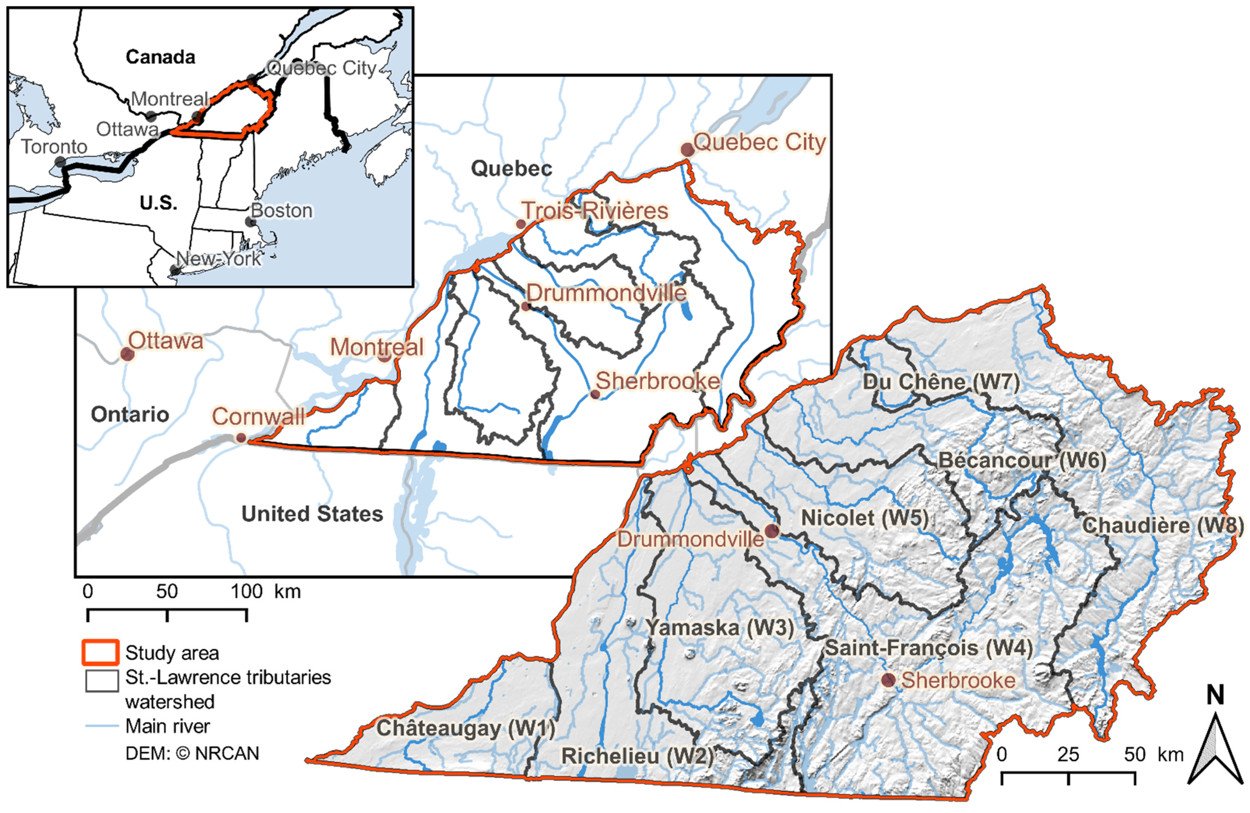
2.1. Study Area
2.2. Simulating Groundwater Recharge with Hydrobudget
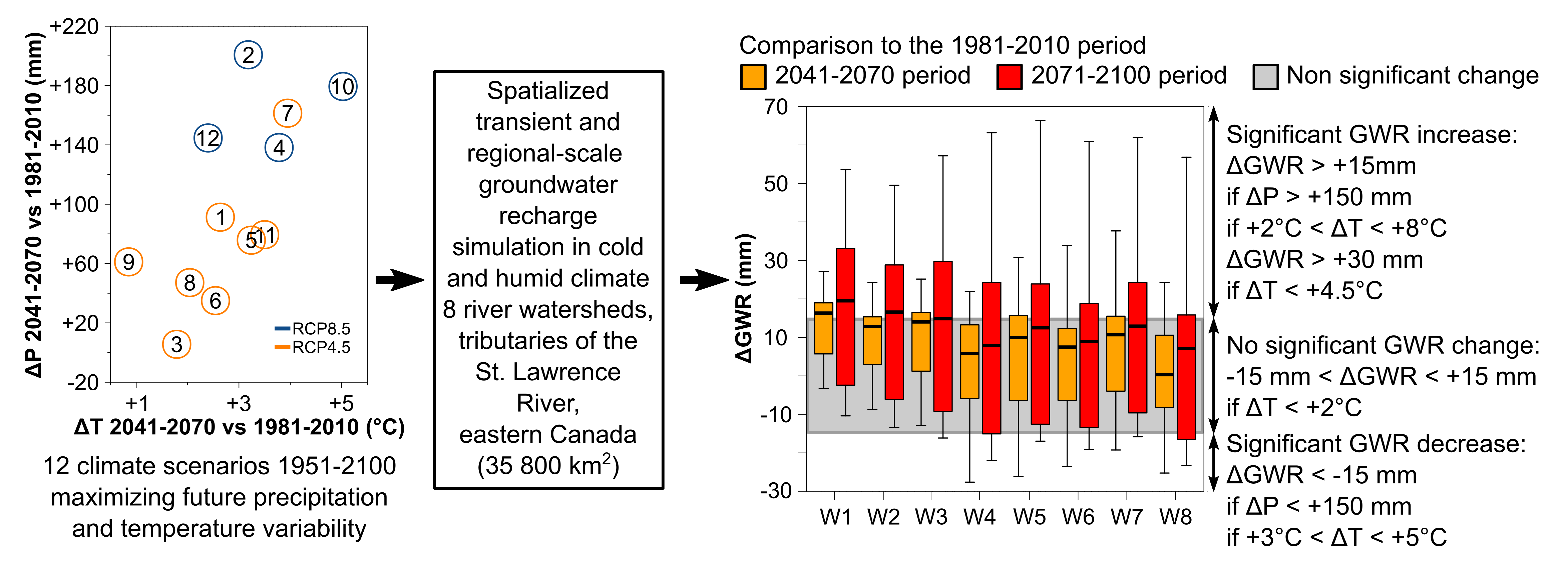
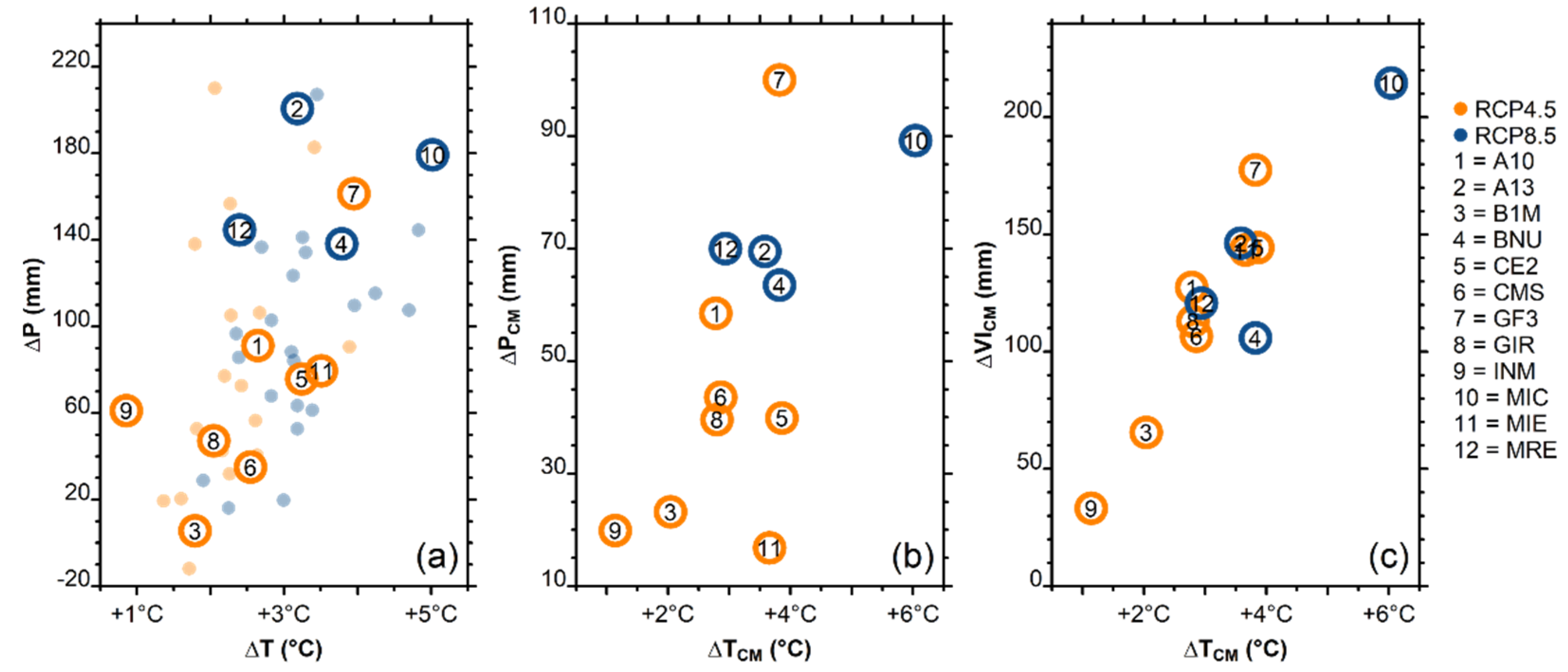
2.3. Climate Scenarios
2.4. Period Comparisons and Significant Changes
3. Results
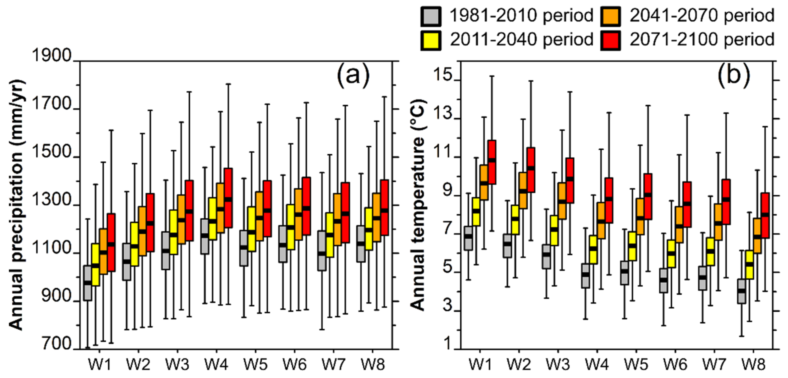
3.1. Climate Changes for the 1981–2100 Period
3.2. Groundwater Recharge for the 1981–2100 Period
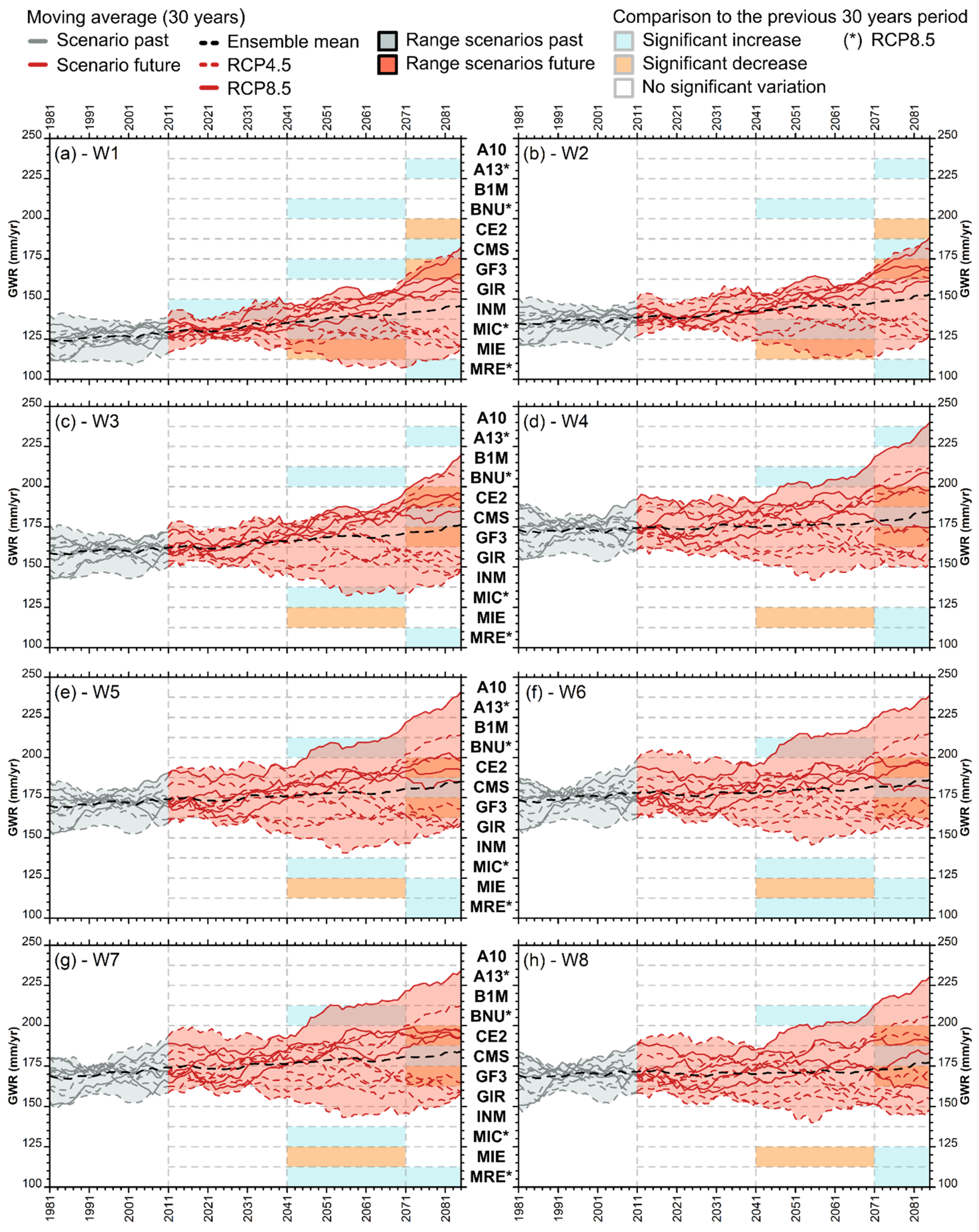
3.3. Inter-Annual Changes in Groundwater Recharge
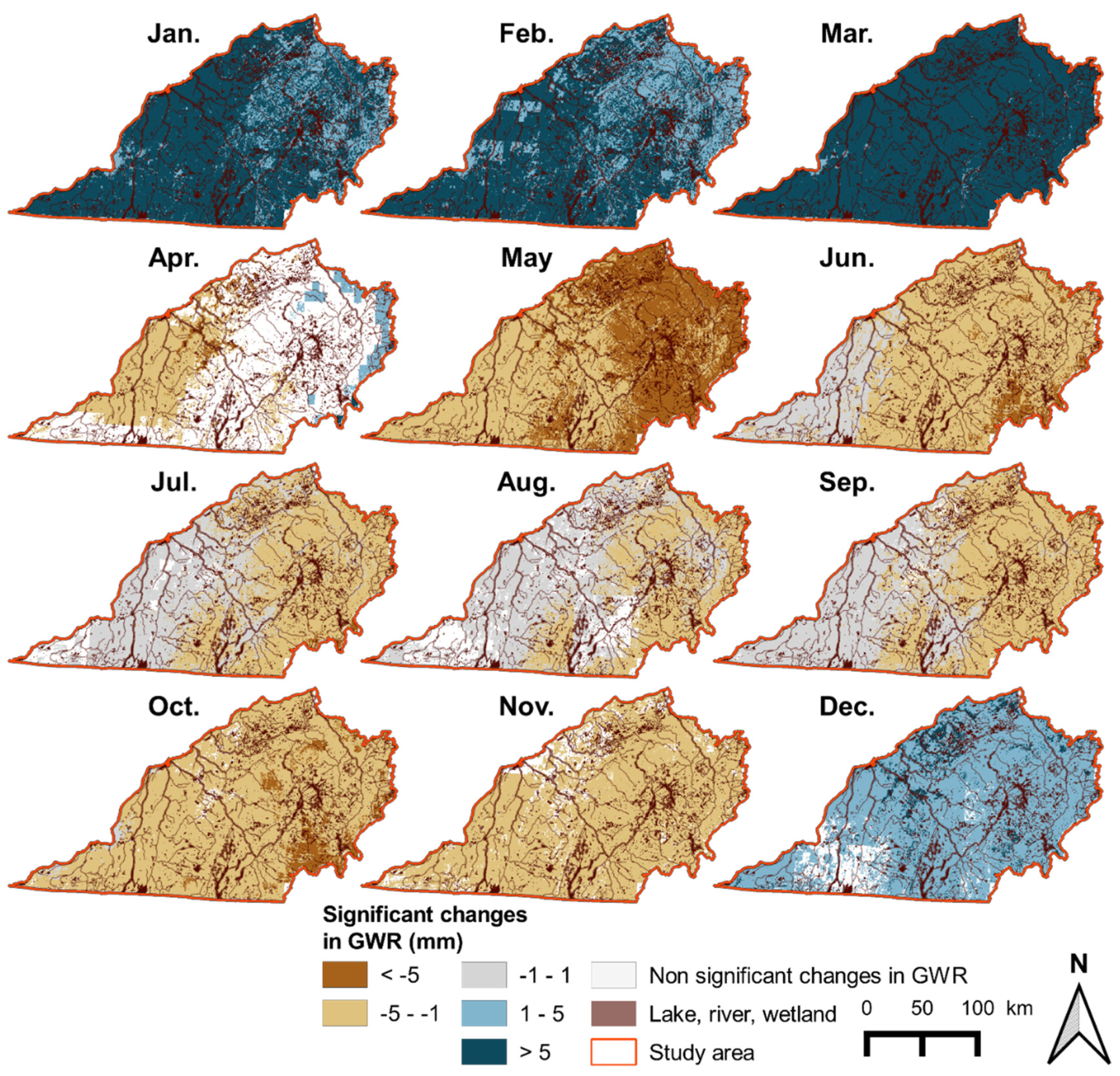
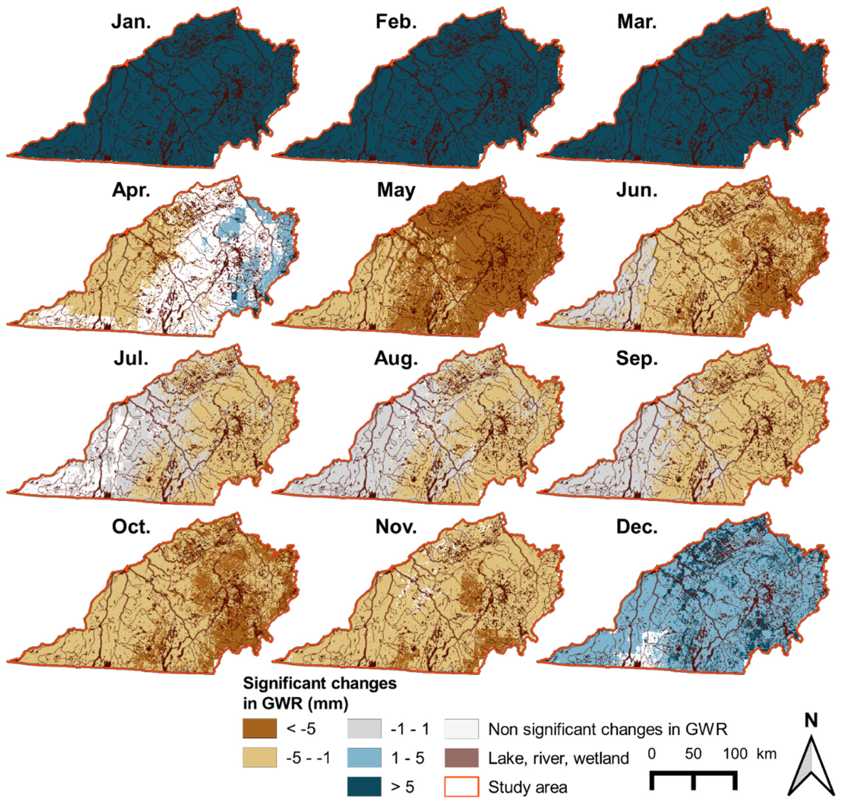
3.4. Spatial Changes in Groundwater Recharge over Time
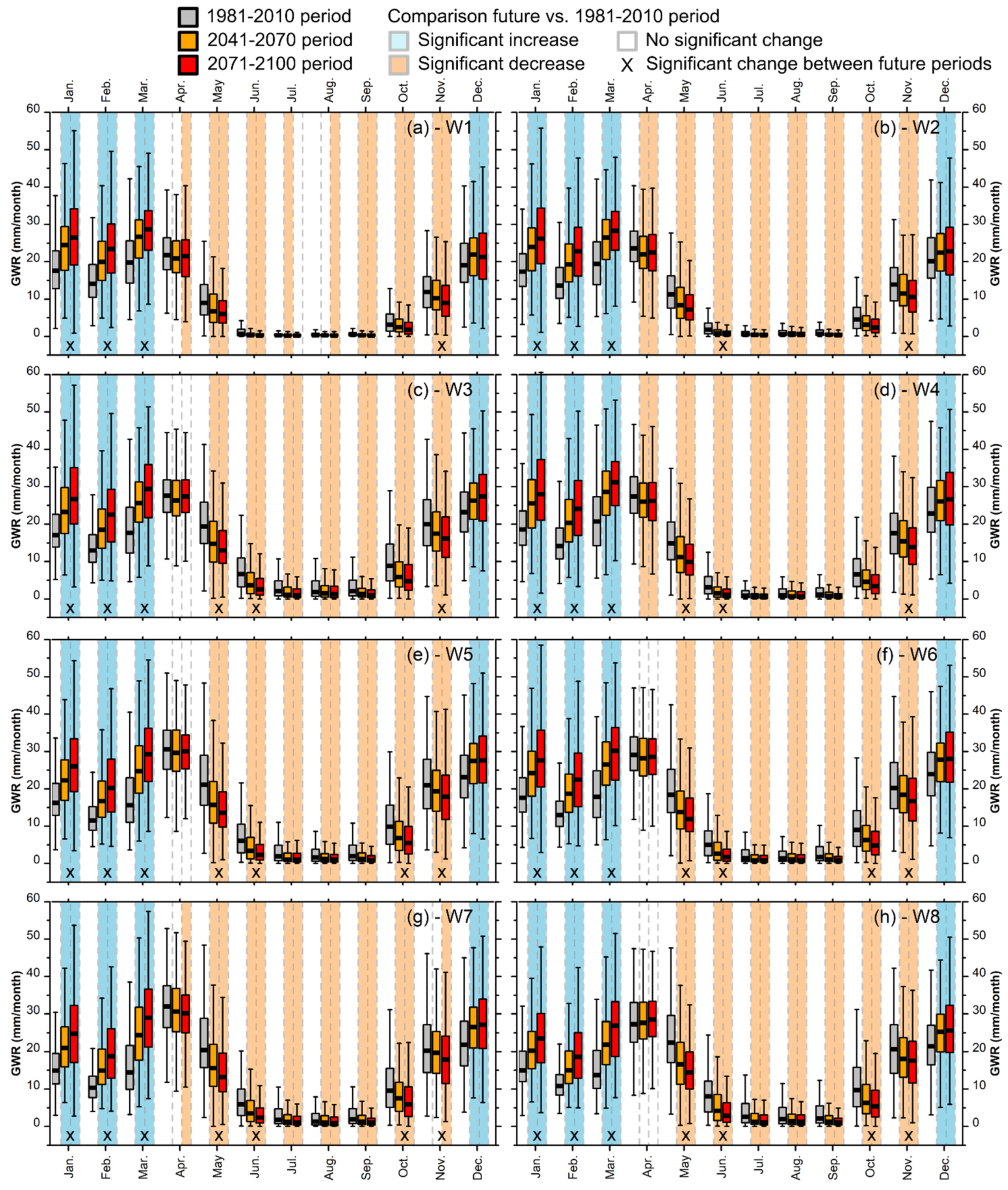
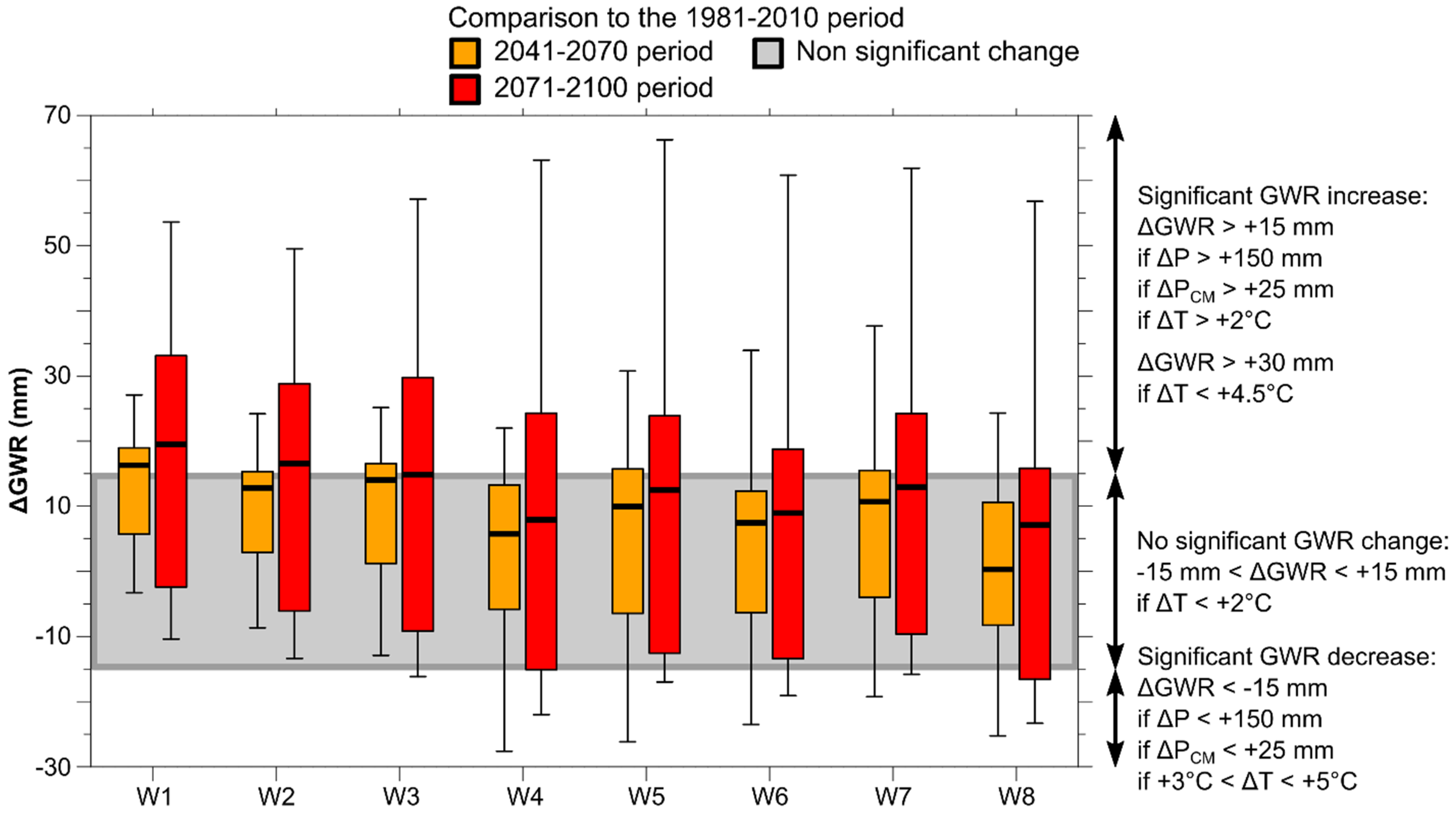
3.5. Monthly Groundwater Recharge Changes over Time
4. Discussion
4.1. Future Groundwater Recharge Dynamics
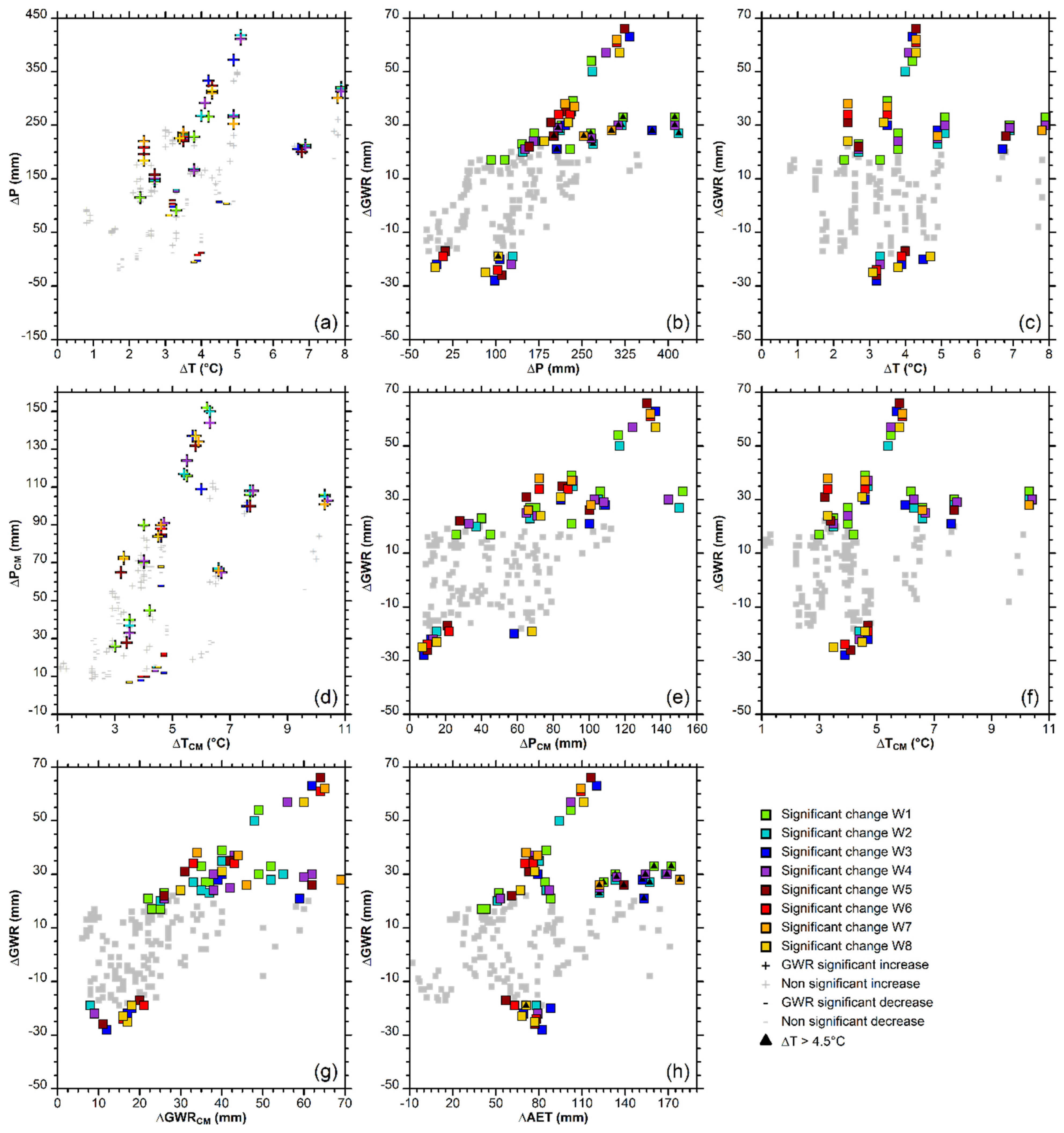
4.2. Climate Changes Impacting Groundwater Recharge
4.3. Future Groundwater Recharge Simulation in Cold and Humid Climates
4.4. Using These Results for Adaptation
5. Conclusions
Author Contributions
Funding
Institutional Review Board Statement
Informed Consent Statement
Data Availability Statement
Acknowledgments
Conflicts of Interest
References
- Gudmundsson, L.; Boulange, J.; Do, H.X.; Gosling, S.N.; Grillakis, M.G.; Koutroulis, A.G.; Leonard, M.; Liu, J.; Schmied, H.M.; Papadimitriou, L.; et al. Globally observed trends in mean and extreme river flow attributed to climate change. Science 2021, 371, 1159–1162. [Google Scholar] [CrossRef]
- Aygün, O.; Kinnard, C.; Campeau, S. Impacts of climate change on the hydrology of northern midlatitude cold regions. Prog. Phys. Geogr. Earth Environ. 2019, 44, 338–375. [Google Scholar] [CrossRef]
- Lee, B.; Hamm, S.-Y.; Jang, S.; Cheong, J.-Y.; Kim, G.-B. Relationship between groundwater and climate change in South Korea. Geosci. J. 2013, 18, 209–218. [Google Scholar] [CrossRef]
- Nygren, M.; Giese, M.; Kløve, B.; Haaf, E.; Rossi, P.M.; Barthel, R. Changes in seasonality of groundwater level fluctuations in a temperate-cold climate transition zone. J. Hydrol. X 2020, 8, 100062. [Google Scholar] [CrossRef]
- Arctic Climate Impact Assessment. Impacts of a Warming Arctic; Cambridge University Press: Cambridge, UK; New York, NY, USA, 2004; ISBN 978-0-521-61778-9. [Google Scholar]
- Döll, P. Vulnerability to the impact of climate change on renewable groundwater resources: A global-scale assessment. Environ. Res. Lett. 2009, 4, 035006. [Google Scholar] [CrossRef]
- Döll, P.; Trautmann, T.; Gerten, D.; Schmied, H.M.; Ostberg, S.; Saaed, F.; Schleussner, C.-F. Risks for the global freshwater system at 1.5 °C and 2 °C global warming. Environ. Res. Lett. 2018, 13, 044038. [Google Scholar] [CrossRef]
- Green, T.R.; Taniguchi, M.; Kooi, H.; Gurdak, J.J.; Allen, D.M.; Hiscock, K.M.; Treidel, H.; Aureli, A. Beneath the surface of global change: Impacts of climate change on groundwater. J. Hydrol. 2011, 405, 532–560. [Google Scholar] [CrossRef] [Green Version]
- Klöve, B.; Ala-Aho, P.; Bertrand, G.; Gurdak, J.J.; Kupfersberger, H.; Kværner, J.; Muotka, T.; Mykrä, H.; Preda, E.; Rossi, P.M.; et al. Climate change impacts on groundwater and dependent ecosystems. J. Hydrol. 2014, 518, 250–266. [Google Scholar] [CrossRef]
- Taylor, R.G.; Scanlon, B.; Döll, P.; Rodell, M.; Van Beek, R.; Wada, Y.; Longuevergne, L.; Leblanc, M.; Famiglietti, J.S.; Edmunds, M.; et al. Ground water and climate change. Nat. Clim. Chang. 2013, 3, 322–329. [Google Scholar] [CrossRef] [Green Version]
- Addor, N.; Rössler, O.; Köplin, N.; Huss, M.; Weingartner, R.; Seibert, J. Robust changes and sources of uncertainty in the projected hydrological regimes of Swiss catchments. Water Resour. Res. 2014, 50, 7541–7562. [Google Scholar] [CrossRef] [Green Version]
- Allen, D.M.; Cannon, A.; Toews, M.; Scibek, J. Variability in simulated recharge using different GCMs. Water Resour. Res. 2010, 46, W00F03. [Google Scholar] [CrossRef]
- Crosbie, R.S.; Pickett, T.; Mpelasoka, F.S.; Hodgson, G.; Charles, S.P.; Barron, O.V. An assessment of the climate change impacts on groundwater recharge at a continental scale using a probabilistic approach with an ensemble of GCMs. Clim. Chang. 2012, 117, 41–53. [Google Scholar] [CrossRef]
- Smerdon, B.D. A synopsis of climate change effects on groundwater recharge. J. Hydrol. 2017, 555, 125–128. [Google Scholar] [CrossRef]
- Larocque, M.; Levison, J.; Martin, A.; Chaumont, D. A review of simulated climate change impacts on groundwater resources in Eastern Canada. Can. Water Resour. J. Rev. Can. Des Ressour. Hydr. 2019, 44, 22–41. [Google Scholar] [CrossRef]
- Moeck, C.; Brunner, P.; Hunkeler, D. The influence of model structure on groundwater recharge rates in climate-change impact studies. Hydrogeol. J. 2016, 24, 1171–1184. [Google Scholar] [CrossRef] [Green Version]
- Reinecke, R.; Schmied, H.M.; Trautmann, T.; Andersen, L.S.; Burek, P.; Flörke, M.; Gosling, S.N.; Grillakis, M.; Hanasaki, N.; Koutroulis, A.; et al. Uncertainty of simulated groundwater recharge at different global warming levels: A global-scale multi-model ensemble study. Hydrol. Earth Syst. Sci. 2021, 25, 787–810. [Google Scholar] [CrossRef]
- Gleeson, T.; Marklund, L.; Smith, L.; Manning, A. Classifying the water table at regional to continental scales. Geophys. Res. Lett. 2011, 38, L05401. [Google Scholar] [CrossRef]
- Kløve, B.; Kvitsand, H.M.L.; Pitkänen, T.; Gunnarsdottir, M.J.; Gaut, S.; Gardarsson, S.; Rossi, P.M.; Miettinen, I. Overview of groundwater sources and water-supply systems, and associated microbial pollution, in Finland, Norway and Iceland. Appl. Hydrogeol. 2017, 25, 1033–1044. [Google Scholar] [CrossRef]
- Meyzonnat, G.; Barbecot, F.; Alazard, M.; McCormack, R. La Richesse de La Ressource En Eau Du Québec (Richness of Quebec’s Water Ressource). Géologues Rev. Off. Société Géologique Fr. 2018, 198, 69–75. [Google Scholar]
- Rivera, A. Canada’s Groundwater Resources; Fitzhenry & Whiteside: Markham, ON, Canada, 2014; ISBN 978-1-55455-292-4. [Google Scholar]
- Dubois, E.; Larocque, M.; Gagné, S.; Meyzonnat, G. Simulation of long-term spatiotemporal variations in regional-scale groundwater recharge: Contributions of a water budget approach in cold and humid climates. Hydrol. Earth Syst. Sci. 2021, 25, 6567–6589. [Google Scholar] [CrossRef]
- Cuthbert, M.O.; Gleeson, T.; Moosdorf, N.; Befus, K.M.; Schneider, A.; Hartmann, J.; Lehner, B. Global patterns and dynamics of climate–groundwater interactions. Nat. Clim. Chang. 2019, 9, 137–141. [Google Scholar] [CrossRef]
- Collins, M.; Knutti, R.; Arblaster, J.; Dufresne, J.-L.; Fichefet, T.; Friedlingstein, P.; Gao, X.; Gutowski, W.J.; Johns, T.; Krinner, G.; et al. Long-term Climate Change: Projections, Commitments and Irreversibility. In Climate Change 2013: The Physical Science Basis. Contribution of Working Group I to the Fifth Assessment Report of the Intergovernmental Panel on Climate Change; Stocker, T.F., Qin, D., Plattner, G.-K., Tignor, M., Allen, S.K., Boschung, J., Nauels, A., Xia, Y., Bex, V., Midgley, P.M., Eds.; Cambridge University Press: Cambridge, UK; New York, NY, USA, 2013; pp. 1029–1136. ISBN 978-1-107-66182-0. [Google Scholar]
- Ouranos. Vers l’adaptation—Synthèse Des Connaissances Sur Les Changements Climatiques Au Québec. (Toward Adaptation—Synthesis on the Knowledge about Climate Change in Quebec), 2015 ed.; Ouranos: Montréal, QC, Canada, 2015; ISBN 978-2-923292-18-2. [Google Scholar]
- Vincent, L.; Zhang, X.; Mekis, E.; Wan, H.; Bush, E. Changes in Canada’s Climate: Trends in Indices Based on Daily Temperature and Precipitation Data. Atmosphere-Ocean 2018, 56, 332–349. [Google Scholar] [CrossRef] [Green Version]
- Arnoux, M.; Brunner, P.; Schaefli, B.; Mott, R.; Cochand, F.; Hunkeler, D. Low-flow behavior of alpine catchments with varying quaternary cover under current and future climatic conditions. J. Hydrol. 2021, 592, 125591. [Google Scholar] [CrossRef]
- Barnett, T.P.; Adam, J.C.; Lettenmaier, D.P. Potential impacts of a warming climate on water availability in snow-dominated regions. Nature 2005, 438, 303–309. [Google Scholar] [CrossRef] [PubMed]
- Berghuijs, W.R.; Woods, R.A.; Hrachowitz, M. A precipitation shift from snow towards rain leads to a decrease in streamflow. Nat. Clim. Chang. 2014, 4, 583–586. [Google Scholar] [CrossRef] [Green Version]
- Cochand, F.; Therrien, R.; Lemieux, J.-M. Integrated Hydrological Modeling of Climate Change Impacts in a Snow-Influenced Catchment. Groundwater 2018, 57, 3–20. [Google Scholar] [CrossRef] [Green Version]
- Hayashi, M.; Farrow, C.R. Watershed-scale response of groundwater recharge to inter-annual and inter-decadal variability in precipitation (Alberta, Canada). Hydrogeol. J. 2014, 22, 1825–1839. [Google Scholar] [CrossRef]
- Scibek, J.; Allen, D.M.; Cannon, A.; Whitfield, P. Groundwater–surface water interaction under scenarios of climate change using a high-resolution transient groundwater model. J. Hydrol. 2007, 333, 165–181. [Google Scholar] [CrossRef]
- Wright, S.N.; Novakowski, K.S. Impacts of warming winters on recharge in a seasonally frozen bedrock aquifer. J. Hydrol. 2020, 590, 125352. [Google Scholar] [CrossRef]
- Dierauer, J.R.; Whitfield, P.H.; Allen, D.M. Climate Controls on Runoff and Low Flows in Mountain Catchments of Western North America. Water Resour. Res. 2018, 54, 7495–7510. [Google Scholar] [CrossRef]
- Jenicek, M.; Seibert, J.; Zappa, M.; Staudinger, M.; Jonas, T. Importance of maximum snow accumulation for summer low flows in humid catchments. Hydrol. Earth Syst. Sci. 2016, 20, 859–874. [Google Scholar] [CrossRef] [Green Version]
- Kong, Y.; Wang, C.-H. Responses and changes in the permafrost and snow water equivalent in the Northern Hemisphere under a scenario of 1.5 °C warming. Adv. Clim. Chang. Res. 2017, 8, 235–244. [Google Scholar] [CrossRef]
- Jyrkama, M.I.; Sykes, J.F. The impact of climate change on spatially varying groundwater recharge in the grand river watershed (Ontario). J. Hydrol. 2007, 338, 237–250. [Google Scholar] [CrossRef]
- Kurylyk, B.L.; MacQuarrie, K.T. The uncertainty associated with estimating future groundwater recharge: A summary of recent research and an example from a small unconfined aquifer in a northern humid-continental climate. J. Hydrol. 2013, 492, 244–253. [Google Scholar] [CrossRef]
- Rivard, C.; Paniconi, C.; Vigneault, H.; Chaumont, D. A watershed-scale study of climate change impacts on groundwater recharge (Annapolis Valley, Nova Scotia, Canada). Hydrol. Sci. J. 2014, 59, 1437–1456. [Google Scholar] [CrossRef] [Green Version]
- Direction De L’expertise Hydrique (DEH) Atlas Hydroclimatique Du Québec Méridional (Hydroclimatic Atlas of Southern Quebec). Available online: https://www.cehq.gouv.qc.ca/atlas-hydroclimatique/Hydraulicite/Qmoy.htm (accessed on 13 April 2021).
- Guay, C.; Minville, M.; Braun, M. A global portrait of hydrological changes at the 2050 horizon for the province of Québec. Can. Water Resour. J. Rev. Can. Des Ressour. Hydr. 2015, 40, 285–302. [Google Scholar] [CrossRef]
- Goderniaux, P.; Brouyère, S.; Blenkinsop, S.; Burton, A.; Fowler, H.; Orban, P.; Dassargues, A. Modeling climate change impacts on groundwater resources using transient stochastic climatic scenarios. Water Resour. Res. 2011, 47, W12516. [Google Scholar] [CrossRef] [Green Version]
- Hund, S.V.; Allen, D.M.; Morillas, L.; Johnson, M.S. Groundwater recharge indicator as tool for decision makers to increase socio-hydrological resilience to seasonal drought. J. Hydrol. 2018, 563, 1119–1134. [Google Scholar] [CrossRef]
- Bertrand, G.; Ponçot, A.; Pohl, B.; Lhosmot, A.; Steinmann, M.; Johannet, A.; Pinel, S.; Caldirak, H.; Artigue, G.; Binet, P.; et al. Statistical hydrology for evaluating peatland water table sensitivity to simple environmental variables and climate changes application to the mid-latitude/altitude Frasne peatland (Jura Mountains, France). Sci. Total. Environ. 2020, 754, 141931. [Google Scholar] [CrossRef]
- Dubois, E.; Larocque, M.; Gagné, S.; Meyzonnat, G. HydroBudget User Guide: Version 1.2; Université du Québec à Montréal, Département des sciences de la Terre et de l’atmosphère: Montréal, QC, Canada, 2021; Available online: https://archipel.uqam.ca/14075/ (accessed on 14 November 2021).
- Dubois, E.; Larocque, M.; Gagne, S.; Meyzonnat, G. HydroBudget—Groundwater Recharge Model in R. Dataverse [Code]. 2021. Available online: https://doi.org/10.5683/SP3/EUDV3H (accessed on 14 November 2021).
- Oudin, L.; Hervieu, F.; Michel, C.; Perrin, C.; Andréassian, V.; Anctil, F.; Loumagne, C. Which potential evapotranspiration input for a lumped rainfall–runoff model? Part 2—Towards a simple and efficient potential evapotranspiration model for rainfall–runoff modelling. J. Hydrol. 2005, 303, 290–306. [Google Scholar] [CrossRef]
- Casajus, N.; Perie, C.; Logan, T.; Lambert, M.-C.; De Blois, S.; Berteaux, D. An Objective Approach to Select Climate Scenarios when Projecting Species Distribution under Climate Change. PLoS ONE 2016, 11, e0152495. [Google Scholar] [CrossRef]
- Hopkinson, R.F.; McKenney, D.W.; Milewska, E.J.; Hutchinson, M.F.; Papadopol, P.; Vincent, L.A. Impact of Aligning Climatological Day on Gridding Daily Maximum–Minimum Temperature and Precipitation over Canada. J. Appl. Meteorol. Clim. 2011, 50, 1654–1665. [Google Scholar] [CrossRef]
- Hutchinson, M.F.; McKenney, D.W.; Lawrence, K.; Pedlar, J.H.; Hopkinson, R.F.; Milewska, E.; Papadopol, P. Development and Testing of Canada-Wide Interpolated Spatial Models of Daily Minimum–Maximum Temperature and Precipitation for 1961–2003. J. Appl. Meteorol. Clim. 2009, 48, 725–741. [Google Scholar] [CrossRef]
- Mpelasoka, F.S.; Chiew, F.H.S. Influence of Rainfall Scenario Construction Methods on Runoff Projections. J. Hydrometeorol. 2009, 10, 1168–1183. [Google Scholar] [CrossRef]
- Sulis, M.; Paniconi, C.; Marrocu, M.; Huard, D.; Chaumont, D. Hydrologic response to multimodel climate output using a physically based model of groundwater/surface water interactions. Water Resour. Res. 2012, 48, W12510. [Google Scholar] [CrossRef] [Green Version]
- Grinevskiy, S.; Pozdniakov, S.; Dedulina, E. Regional-Scale Model Analysis of Climate Changes Impact on the Water Budget of the Critical Zone and Groundwater Recharge in the European Part of Russia. Water 2021, 13, 428. [Google Scholar] [CrossRef]
- Luoma, S.; Okkonen, J. Impacts of Future Climate Change and Baltic Sea Level Rise on Groundwater Recharge, Groundwater Levels, and Surface Leakage in the Hanko Aquifer in Southern Finland. Water 2014, 6, 3671–3700. [Google Scholar] [CrossRef] [Green Version]
- Rathay, S.; Allen, D.; Kirste, D. Response of a fractured bedrock aquifer to recharge from heavy rainfall events. J. Hydrol. 2018, 561, 1048–1062. [Google Scholar] [CrossRef] [Green Version]
- Sulis, M.; Paniconi, C.; Rivard, C.; Harvey, R.; Chaumont, D. Assessment of climate change impacts at the catchment scale with a detailed hydrological model of surface-subsurface interactions and comparison with a land surface model. Water Resour. Res. 2011, 47, W01513. [Google Scholar] [CrossRef]
- Prein, A.F.; Rasmussen, R.M.; Ikeda, K.; Liu, C.; Clark, M.P.; Holland, G.J. The future intensification of hourly precipitation extremes. Nat. Clim. Chang. 2016, 7, 48–52. [Google Scholar] [CrossRef]
- Nemri, S.; Kinnard, C. Comparing calibration strategies of a conceptual snow hydrology model and their impact on model performance and parameter identifiability. J. Hydrol. 2019, 582, 124474. [Google Scholar] [CrossRef]
- Melsen, L.A.; Guse, B. Climate change impacts model parameter sensitivity—Implications for calibration strategy and model diagnostic evaluation. Hydrol. Earth Syst. Sci. 2021, 25, 1307–1332. [Google Scholar] [CrossRef]
- Jaramillo, F.; Prieto, C.; Lyon, S.W.; Destouni, G. Multimethod assessment of evapotranspiration shifts due to non-irrigated agricultural development in Sweden. J. Hydrol. 2013, 484, 55–62. [Google Scholar] [CrossRef] [Green Version]
- Destouni, G.; Jaramillo, F.; Prieto, C. Hydroclimatic shifts driven by human water use for food and energy production. Nat. Clim. Chang. 2012, 3, 213–217. [Google Scholar] [CrossRef]
- Guerrero-Morales, J.; Fonseca, C.; Goméz-Albores, M.; Sampedro-Rosas, M.; Silva-Gómez, S. Proportional Variation of Potential Groundwater Recharge as a Result of Climate Change and Land-Use: A Study Case in Mexico. Land 2020, 9, 364. [Google Scholar] [CrossRef]
- Verburg, P.H.; Neumann, K.; Nol, L. Challenges in using land use and land cover data for global change studies. Glob. Chang. Biol. 2011, 17, 974–989. [Google Scholar] [CrossRef] [Green Version]
- Koirala, S.; Jung, M.; Reichstein, M.; De Graaf, I.; Camps-Valls, G.; Ichii, K.; Papale, D.; Ráduly, B.; Schwalm, C.R.; Tramontana, G.; et al. Global distribution of groundwater-vegetation spatial covariation. Geophys. Res. Lett. 2017, 44, 4134–4142. [Google Scholar] [CrossRef]
- Groupe Agéco. Recherche Participative D’alternatives Durables Pour La Gestion De L’eau En Milieu Agricole Dans Un Contexte De Changement Climatique (RADEAU1) (Participative Research for Sustainable Options in Water Management in Agricole Region and within a Climate Change Context); Ministère de l’agriculture, des pêcheries et de l’alimentation, Fonds Vert: Quebec City, QC, Canada, 2019; p. 332. Available online: https://www.agrireseau.net/documents/Document_101346.pdf (accessed on 14 November 2021).


| Area (km2) | Median Elevation (m asl) | Annual | Cold Months | Pot. GWR | |||||||
|---|---|---|---|---|---|---|---|---|---|---|---|
| T (°C) | P (mm) | T (°C) | VI (mm) | mm/yr | Win. | Spr. | Sum. | Fall | |||
| W1. Châteaugay * | 2219 | 51 | 6.5 | 952 | −6.4 | 211 | 109 | 38% | 46% | 3% | 14% |
| W2. Richelieu * | 4414 | 40 | 6.3 | 1039 | −6.7 | 223 | 119 | 36% | 45% | 4% | 15% |
| W3. Yamaska | 4792 | 80 | 5.9 | 1080 | −7.1 | 231 | 139 | 35% | 44% | 4% | 17% |
| W4. Saint-François * | 9068 | 312 | 4.8 | 1123 | −7.8 | 214 | 147 | 31% | 42% | 8% | 19% |
| W5. Nicolet | 3591 | 150 | 5.1 | 1076 | −8.0 | 196 | 144 | 32% | 43% | 6% | 19% |
| W6. Bécancour | 3380 | 140 | 4.5 | 1103 | −8.7 | 164 | 151 | 28% | 44% | 7% | 21% |
| W7. Du Chêne | 461 | 90 | 4.5 | 1092 | −8.9 | 142 | 154 | 26% | 46% | 8% | 20% |
| W8. Chaudière | 7879 | 340 | 3.9 | 1092 | −8.9 | 151 | 145 | 27% | 42% | 10% | 21% |
| Parameter | Regionally Calibrated Value from Dubois et al. [22] | ||
|---|---|---|---|
| Snowmelt model | Melting temperature—TM (°C) | Air temperature threshold for snowmelt | 1.4 |
| Melting coefficient—CM (mm/°C/d) | Melting rate of the snowpack | 4.9 | |
| Freezing soil conditions | Threshold temperature for soil frost—TTF (°C) | Air temperature threshold for soil frost | −15.9 |
| Freezing time—FT (d) | Duration of air temperature threshold to freeze the soil | 16.4 | |
| Runoff | Antecedent precipitation index time—tAPI (d) | Time constant to consider the soil in dry or wet conditions based on previous precipitation event | 3.9 |
| Runoff factor—frunoff (-) | Correction factor for runoff computed with the RCN method for the partitioning between runoff and infiltration into the soil reservoir | 0.60 | |
| Lumped soil reservoir | Maximum soil water content—swm (mm) | Soil reservoir storage capacity, maximum height of water stored in a 1 m soil profile | 385 |
| Infiltration factor—finf (-) | Fraction of soil water that produces deep percolation at each daily time step | 0.06 | |
| Name. | Model Source | Code | RCP |
|---|---|---|---|
| ACCESS1-0_rcp45_r1i1p1 | Commonwealth Scientific and Industrial Research Organization (CSIRO), Australia and Bureau of Meteorology (BOM), Australia | A10 | 4.5 |
| ACCESS1-3_rcp85_r1i1p1 | Commonwealth Scientific and Industrial Research Organization (CSIRO), Australia and Bureau of Meteorology (BOM), Australia | A13 | 8.5 |
| bcc-csm1-1-m_rcp45_r1i1p1 | Beijing Climate Center, China Meteorological Administration, China | B1M | 4.5 |
| BNU-ESM_rcp85_r1i1p1 | College of Global Change and Earth System Science, Beijing Normal University (BNU), China | BNU | 8.5 |
| CanESM2_rcp45_r1i1p1 | Canadian Center for Climate Modelling and Analysis (CCCma), Canada | CE2 | 4.5 |
| CMCC-CMS_rcp45_r1i1p1 | Centro Euro-Mediterraneo sui Cambiamenti Climatici Climate Model, Italy | CMS | 4.5 |
| GFDL-CM3_rcp45_r1i1p1 | Geophysical Fluid Dynamics Laboratory (GFDL), USA | GF3 | 4.5 |
| GISS-E2-R_rcp45_r6i1p3 | National Aeronautics and Space Administration (NASA)/Goddard Institute for Space Studies (GISS), USA | GIR | 4.5 |
| inmcm4_rcp45_r1i1p1 | Institute for Numerical Mathematics (INM), Russia | INM | 4.5 |
| MIROC-ESM _rcp45_r1i1p1 | Japan Agency for Marine-Earth Science and Technology, Atmosphere and Ocean Research Institute (The University of Tokyo), National Institute for Environmental Studies, Japan | MIC | 8.5 |
| MIROC-ESM-CHEM_rcp85_r1i1p1 | Japan Agency for Marine-Earth Science and Technology, Atmosphere and Ocean Research Institute (The University of Tokyo), National Institute for Environmental Studies, Japan | MIE | 4.5 |
| MRI-ESM1_rcp85_r1i1p1 | Meteorological Research Institute, Japan | MRE | 8.5 |
| W1 | W2 | W3 | W4 | W5 | W6 | W7 | W8 | |||||||||
|---|---|---|---|---|---|---|---|---|---|---|---|---|---|---|---|---|
| CM | WM | CM | WM | CM | WM | CM | WM | CM | WM | CM | WM | CM | WM | CM | WM | |
| 1981–2010 | 126 (26) | 136 (24) | 160 (26) | 173 (28) | 171 (26) | 175 (28) | 170 (28) | 170 (24) | ||||||||
| 74 | 31 | 74 | 39 | 80 | 53 | 75 | 71 | 77 | 66 | 71 | 74 | 66 | 72 | 66 | 77 | |
| 2011–2040 | 132 (22) | 140 (22) | 164 (26) | 175 (34) | 175 (34) | 177 (38) | 175 (36) | 171 (36) | ||||||||
| 82 | 27 | 82 | 33 | 89 | 45 | 85 | 61 | 86 | 57 | 81 | 64 | 77 | 64 | 75 | 67 | |
| 2041–2070 | 138 (42) | 145 (42) | 168 (48) | 176 (54) | 178 (60) | 180 (60) | 178 (60) | 171 (50) | ||||||||
| 93 | 25 | 93 | 30 | 102 | 41 | 96 | 54 | 99 | 51 | 94 | 57 | 90 | 58 | 85 | 58 | |
| 2071–2100 | 143 (60) | 150 (60) | 173 (68) | 181 (76) | 182 (78) | 183 (76) | 182 (76) | 175 (74) | ||||||||
| 101 | 22 | 102 | 27 | 112 | 36 | 107 | 48 | 110 | 45 | 105 | 50 | 102 | 50 | 97 | 51 | |
| Climate Scenario | Period ** | Precipitation (mm) and Temperature (°C) Changes Compared to Previous 30-Year Period | |||||||||||||||
|---|---|---|---|---|---|---|---|---|---|---|---|---|---|---|---|---|---|
| W1 | W2 | W3 | W4 | W5 | W6 | W7 | W8 | ||||||||||
| ΔP | ΔT | ΔP | ΔT | ΔP | ΔT | ΔP | ΔT | ΔP | ΔT | ΔP | ΔT | ΔP | ΔT | ΔP | ΔT | ||
| A13 * | 3 | 198 | 1.9 | 200 | 1.9 | 113 | 1.8 | 191 | 1.9 | ||||||||
| BNU * | 2 | 119 | 2.6 | 121 | 2.6 | 39 | 1.1 | 121 | 2.6 | 116 | 2.6 | 118 | 2.6 | 119 | 2.6 | 40 | 1.1 |
| CE2 | 3 | −45 | 0.7 | −47 | 0.7 | 34 | 1.6 | −47 | 0.7 | −36 | 0.7 | −30 | 0.7 | 13 | 1.6 | ||
| CMS | 3 | 180 | 0.9 | 183 | 0.9 | −39 | 1.0 | 181 | 0.9 | 179 | 1.0 | 184 | 1.0 | 188 | 1.0 | −38 | 1.0 |
| GF3 | 2 | 92 | 2.1 | ||||||||||||||
| GF3 | 3 | −57 | 0.7 | −60 | 0.7 | 79 | 2.1 | −63 | 0.7 | −60 | 0.8 | −48 | 0.8 | −51 | 0.8 | 61 | 2.3 |
| INM | 1 | 36 | 0.2 | ||||||||||||||
| MIC * | 2 | 176 | 2.8 | 182 | 2.8 | 68 | 2.2 | 158 | 2.8 | 145 | 2.7 | 176 | 2.8 | ||||
| MIE | 2 | −11 | 1.6 | −16 | 1.6 | 94 | 1.7 | −18 | 1.6 | −4 | 1.5 | 8 | 1.5 | −15 | 1.6 | 60 | 1.7 |
| MIE | 3 | −6 | 1.2 | 16 | 1.2 | 35 | 1.2 | 25 | 1.4 | ||||||||
| MRE * | 2 | 117 | 1.5 | 120 | 1.5 | ||||||||||||
| MRE * | 3 | 135 | 1.9 | 144 | 1.9 | 88 | 1.5 | 146 | 1.9 | 127 | 1.9 | 100 | 1.9 | 88 | 1.9 | 104 | 1.5 |
| W1 | W2 | W3 | W4 | W5 | W6 | W7 | W8 | |
|---|---|---|---|---|---|---|---|---|
| 2041–2070 | 5 [2] | 3 [2] | 1 [0] | 3 [2] | 2 [1] | 2 [1] | 2 [2] | 2 [1] |
| 2071–2100 | 6 [4] | 6 [4] | 6 [3] | 6 [4] | 5 [2] | 3 [1] | 3 [2] | 4 [1] |
Publisher’s Note: MDPI stays neutral with regard to jurisdictional claims in published maps and institutional affiliations. |
© 2022 by the authors. Licensee MDPI, Basel, Switzerland. This article is an open access article distributed under the terms and conditions of the Creative Commons Attribution (CC BY) license (https://creativecommons.org/licenses/by/4.0/).
Share and Cite
Dubois, E.; Larocque, M.; Gagné, S.; Braun, M. Climate Change Impacts on Groundwater Recharge in Cold and Humid Climates: Controlling Processes and Thresholds. Climate 2022, 10, 6. https://doi.org/10.3390/cli10010006
Dubois E, Larocque M, Gagné S, Braun M. Climate Change Impacts on Groundwater Recharge in Cold and Humid Climates: Controlling Processes and Thresholds. Climate. 2022; 10(1):6. https://doi.org/10.3390/cli10010006
Chicago/Turabian StyleDubois, Emmanuel, Marie Larocque, Sylvain Gagné, and Marco Braun. 2022. "Climate Change Impacts on Groundwater Recharge in Cold and Humid Climates: Controlling Processes and Thresholds" Climate 10, no. 1: 6. https://doi.org/10.3390/cli10010006