Not p-Values, Said a Little Bit Differently


Department of Economics, University of California, Santa Barbara, CA 93106, USA
Econometrics 2019, 7(1), 11; https://doi.org/10.3390/econometrics7010011
Submission received: 14 December 2018
/
Revised: 25 February 2019
/
Accepted: 7 March 2019
/
Published: 13 March 2019
(This article belongs to the Special Issue Towards a New Paradigm for Statistical Evidence)
Abstract
:As a contribution toward the ongoing discussion about the use and mis-use of p-values, numerical examples are presented demonstrating that a p-value can, as a practical matter, give you a really different answer than the one that you want.
1. Introduction
The American Statistical Association statement on “Statistical Significance and P-values” (Wasserstein and Lazar 2016) aimed at reminding the statistics community about a number of pitfalls that are commonly fallen into, in the everyday use of p-values. The statement and accompanying introduction also pointed to the rich history of the statisticians who have articulated the issues, providing a long list of references. This raises a question: If no one has listened before, will they be swayed by this latest exhortation? Perhaps a numerical example might be more convincing—an example that illustrates that the issue is less that the common use of p-values is philosophically misguided, and more that the numbers can just be completely wrong (for evidence that these issues are of real, applied importance in economics and finance see Kim and Ji (2015).
One way in which to understand the misuse of the p-value is as a misapplication of the modus tollens argument. Suppose we had data that would prove a null hypothesis to be true or false, with certainty. If the null hypothesis is true, then the data would support the null with certainty. So if the data did not support the null, we would know that the null is false. However, such logic does not apply to statistical reasoning, where the data does not give answers with certainty. If the null is true, then a small p-value is unlikely. The fallacy of applying modus tollens is that it may be that if the null is false, then a small p-value is also unlikely.
Problems with the misuse of p-values have been understand for a very long time—at least in principle. The purpose here is to provide a new-but-simple example of the disconnect between a p-value and the probability that a null hypothesis is true—adding to the long list of existing examples. Beginning with a quick review of what has been said in the past may be useful. There are a number of concerns with regard to p-values, which have been discussed at least as far back as Berkson (1942), and as recently as Wasserstein and Lazar (2016). The latter also includes many references. I focus here solely on the issue that a p-value is not designed to speak to the relative merits of a null hypothesis versus the alternative. Nickerson (2000) explains the problem, and gives many further references. Trafimow (2003) puts the matter succinctly, “although one can calculate the probability of obtaining a finding given that the null hypothesis is true, this is not equivalent to calculating the probability that the null hypothesis is true given that one has obtained a finding.”1 Trafimow (2005) is more pointed, writing, “A p-value can be a dramatic overestimate or underestimate of the desired posterior probability of the null hypothesis depending on the prior probability of the null hypothesis and the probability of the finding given that the null hypothesis is not true.”
Dickey (1977) points out that the area under the tail is not, in general, a good approximation to the Bayes factor. Berger and Sellke (1987) summarize the issue nicely, writing that “actual evidence against a null (as measured, say, by posterior probability or comparative likelihood) can differ by an order of magnitude from the p-value. … The overall conclusion is that p-values can be highly misleading measures of the evidence provided by the data against the null hypothesis” Trafimow and Rice (2009) show that the p-value need not even be very highly correlated with the true probability of the null hypothesis.
The point addressed here is the ASA’s second principle, “P-values do not measure the probability that the studied hypothesis is true…” Or as E.S. Pearson (1938) wrote eight decades ago, “Gosset … had a tremendous influence on the … idea which has formed the basis of all the…researches of Neyman and myself. It is the simple suggestion that the only valid reason for rejecting a statistical hypothesis is that some alternative hypothesis explains the events with a greater degree of probability.” Hubbard and Bayarri (2003) explain the difference between Fisher’s advocacy of the p-value and the idea of Neyman and Pearson to compare a null hypothesis to an alternative, offering historical perspectives as well. Robinson and Wainer (2002) discuss a number of issues with the use of p-values, including the point that “… many users of NHST [Null Hypothesis Significance Testing] interpret the result as the probability of the null hypothesis based on the data observed. … This error suggests that users really want to make a different kind of inference—a probabilistic statement of the likelihood of the hypothesis”, which is the point that we pursue below.2 Hubbard and Lindsay (2008) write that “P-Values Exaggerate the Evidence Against the Null Hypothesis”. This is the most damning criticism of the p-value as a measure of evidence.” (Emphasis in the original). We shall see, however, that it is also possible for a p-value to understate the evidence against the null.
2. The General Problem
Wasserstein and Lazar (2016) succinctly remind everyone that “Informally, a p-value is the probability under a specified statistical model that a statistical summary of the data … would be equal to or more extreme than its observed value.” Following Trafimow (2005), suppose that we call finding that probability to be equal to or more extreme to be the “finding”, or simply, . The “philosophical” problem is that p-values summarize , while we are, with rare exception, interested in . The two are related by Bayes’ Theorem, but they are not the same. Pointedly, they need not even be close. As a reminder, the p-value is calculated by assuming that the null hypothesis is true, and then calculating the probability that some observed outcome would come about under the null hypothesis. The classic case is to calculate the probability that an estimated parameter should be as far or farther from a point that is specified by the null, as is the observed estimate. The p-value is , but from Bayes’ theorem:
The generic reason that the p-value need not be close to the conditional probability of the hypothesis is that the p-value is missing the other two elements in Equation (1). Since this is obvious, it is probably worth commenting on why the deployment of the p-value remains nearly pervasive. The requirement to specify is sometimes viewed as non-scientific, as it comes from something other than the data at hand. Also, the specification of generally requires considerable information about the alternative hypothesis, certainly much more than merely the idea that the alternative is anything other than the null.
The notion that the p-value summarizes is an oversimplification, of course, as it ignores conditioning on the econometric specification of the entire estimate. Really, the p-value gives . Conditioning on specification carries through to the left side of Equation (1), but in what follows, I will omit it for the sake of brevity. In addition, when one applies Bayes’ Theorem, the result is really conditioned on the prior specified, although this is traditionally omitted from the notation. It is also true that frequentists and Bayesians sometimes disagree over the entire nature of the statistical enterprise, including even the meaning of “probability.” Nothing in what follows speaks to these deeper issues.
3. A Simple Example of the Problem
Consider the decision of whether a coin is fair or not, based on the number of heads, , observed after tosses. If there are 26 heads out of 64 tosses, the p-value is 0.08 (so the null seems very unlikely). Though a bit short of the magic number 0.05, that’s a sufficiently low p-value that a sympathetic editor might consider publication. Doing the Bayes’ Theorem calculation requires some additional assumptions, but arguably innocuous assumptions suggest that the coin is more likely than not, fair, —a strikingly different conclusion (“Arguably innocuous” being taken here as the prior odds for the coin being fair being 50/50, and that if the coin is not fair, all we know is that the probability of a head is between zero and one). Note that since the posterior is not far from the prior, we would conclude that the data is not very informative, which is probably not the conclusion one would draw from looking at the 0.08 p-value.
In this example, the studied hypothesis is that the mean chance of a head is , and that the p-value is , where is the cdf (cumulative distribution function) of the binomial distribution. Bayes Theorem gives us as a function of the binomial probability mass function , and a prior over , .
Unlike the formula for calculating the p-value, here, the answer requires some extra inputs. Most researchers would probably agree that the probability of a head is between zero and one, so that outside that range, equals zero. Beyond that, we probably want to put some finite mass onto the studied hypothesis. might be thought of as neutral.3 Also, we might be as ignorant as possible about alternative values, by spreading the rest of the mass uniformly between the limits, so between zero and one, . This gives:
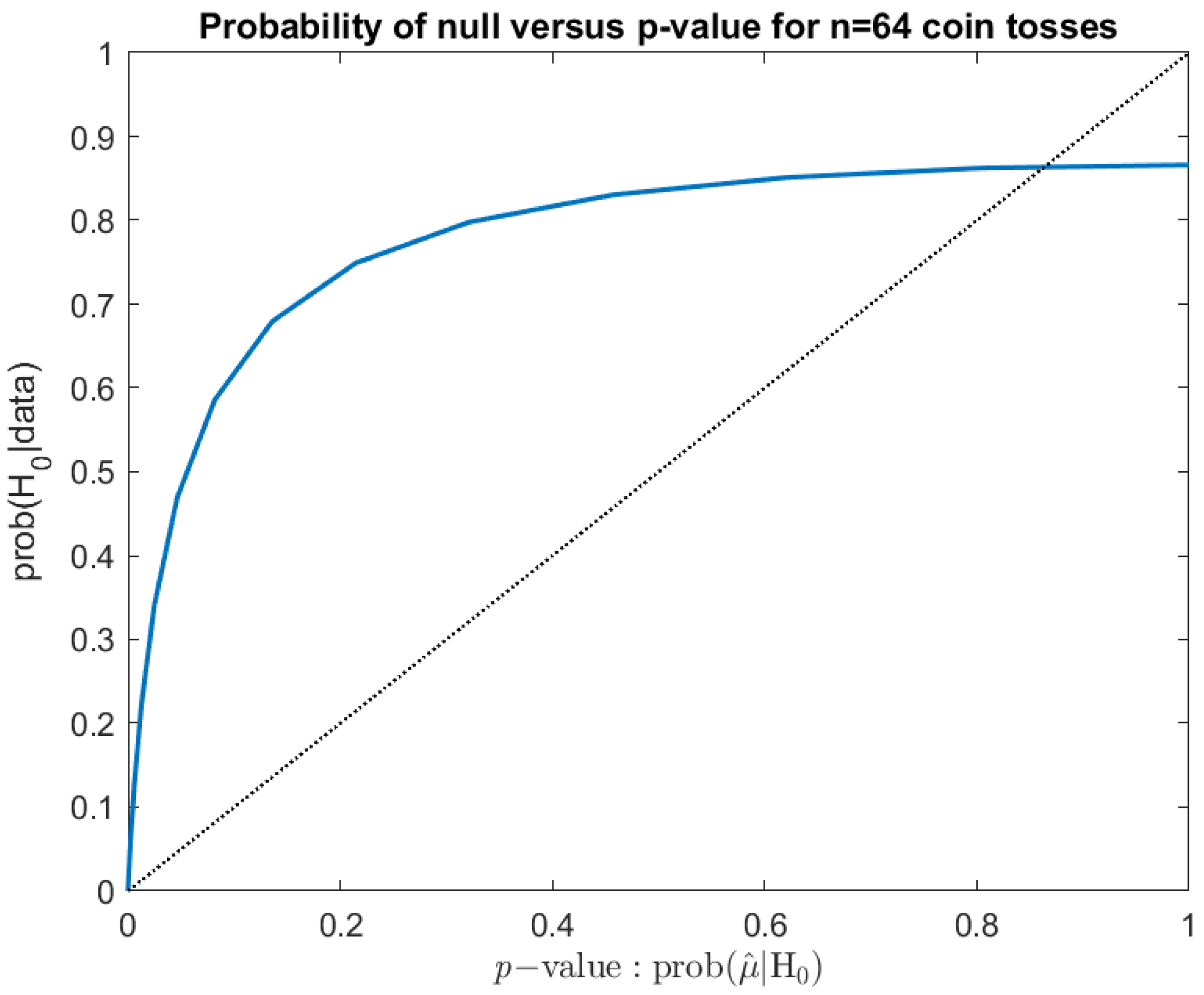
Using these assumptions gives us the value given above. Of course, varying counts of heads give different probabilities and p-values, with the relation between the two for the 64 coin tosses shown in Figure 1. If the p-value gave the probability that the hypothesis were true, the plot would lie along the 45° line. However, it does not do so. Regardless, the more important lesson is that the curve is often very far from the 45° line, and indeed, it can lie either above or below.
Different priors do give different probabilities for the studied hypothesis, so there may well be a prior for which the p-value does coincide with the correct probability for the studied hypothesis. In the example here, if we put a prior weight, , on the fair coin that is equal to 0.04, we obtain a probability that is equal to the 0.08 p-value. Still, it seems likely that a p-valuista who rejects a fair coin did not intend to declare a prior of 96 percent against the coin being fair.
4. Summary
The point in the ASA statement is not that p-values give the wrong answer; the point is that p-values usually commit what (Howard Raiffa (1968), attributing the idea to John Tukey) called “errors of the third kind: solving the wrong problem.” Not always, of course. For example, in a capital punishment case, we might well be interested only in controlling for Type I error against a null of not guilty, as distinct from deciding whether the accused is innocent or guilty. But in most cases, we do care about what the data tells us with regard to the probability of the studied hypothesis. As a practical matter, the p-value cannot be expected to be a good guide for this probability.
Funding
This research received no external funding.
Acknowledgments
Conflicts of Interest
The author declares no conflict of interest.
References
- Berger, James O., and Thomas Sellke. 1987. Testing a Point Null Hypothesis: The Irreconcilability of P Values and Evidence (with comments). Journal of the American Statistical Association 82: 112–39. [Google Scholar] [CrossRef]
- Berkson, Joseph. 1942. Tests of Significance Considered as Evidence. Journal of the American Statistical Association 37: 325–35. [Google Scholar] [CrossRef]
- Dickey, James M. 1977. Is the Tail Area Useful as an Approximate Bayes Factor? Journal of the American Statistical Association 72: 138–42. [Google Scholar] [CrossRef]
- Hubbard, Raymond, and María Jesús Bayarri. 2003. Confusion over Measures of Evidence (p’s) versus Errors (α’s) in Classical Statistical Testing. American Statistician 57: 171–82, Comments by K. N. Berk and M. A. Carlton, and Rejoinder. [Google Scholar] [CrossRef]
- Hubbard, Raymond, and R. Murray Lindsay. 2008. Why P-Values Are Not a Useful Measure of Evidence in Statistical Significance Testing. Theory & Psychology 18: 69–88. [Google Scholar]
- Kim, Jae H., and Philip Inyeob Ji. 2015. Significance testing in empirical finance: A critical review and assessment. Journal of Empirical Finance 34: 1–14. [Google Scholar] [CrossRef]
- Nickerson, Raymond S. 2000. Null hypothesis significance testing: A review of an old and continuing controversy. Psychological Methods 5: 241–301. [Google Scholar] [CrossRef] [PubMed]
- Pearson, Egon S. 1938. “Student” as a statistician. Biometrika 30: 210–50. [Google Scholar] [CrossRef]
- Raiffa, Howard. 1968. Decision Analysis: Introductory Lectures on Choices under Uncertainty. Reading: Addison-Wesley. [Google Scholar]
- Robinson, Daniel H., and Howard Wainer. 2002. On the Past and Future of Null Hypothesis Significance Testing. Journal of Wildlife Management 66: 262–71. [Google Scholar] [CrossRef]
- Startz, Richard. 2014. Choosing the More Likely Hypothesis. Foundations and Trends in Econometrics 7: 120–86. [Google Scholar] [CrossRef]
- Trafimow, David. 2003. Hypothesis Testing and Theory Evaluation at the Boundaries: Surprising Insights From Bayes’s Theorem. Psychological Review 110: 526–35. [Google Scholar] [CrossRef] [PubMed]
- Trafimow, David. 2005. The ubiquitous Laplacian assumption: Reply to Lee and Wagenmakers. Psychological Review 112: 669–74. [Google Scholar] [CrossRef]
- Trafimow, David. 2015. The benefits of applying Bayes’ theorem in medicine. American Research Journal of Humanities and Social Sciences 1: 14–23. [Google Scholar]
- Trafimow, David, and Michael Marks. 2015. Editorial. Basic and Applied Social Psychology 37: 1–2. [Google Scholar] [CrossRef]
- Trafimow, David, and Stephen Rice. 2009. A test of the NHSTP correlation argument. Journal of General Psychology 136: 261–69. [Google Scholar] [CrossRef] [PubMed]
- Wasserstein, Ronald L., and Nicole A. Lazar. 2016. The ASA’s Statement on p-Values: Context, Process, and Purpose. The American Statistician 70: 129–33. [Google Scholar] [CrossRef]
| 1 | See also Trafimow (2015) and Trafimow and Marks (2015). Trafimow offers a bit of history and explanations that are suitable for students at https://www.youtube.com/watch?v=dsp_hSIsacQ. |
| 2 | Robinson and Wainer (2002) take a more sanguine view of the possible damage of conflating the Fisherian and Neyman–Pearson approaches than does Hubbard and Bayarri (2003). |
| 3 | A dedicated Bayesian might point out that in the presence of prior information, a relatively non-informative prior would not be appropriate. An informative prior might lead to , either closer to the p-value or farther away. |
Figure 1.
Relation between probability of the null and the p-value for various observed heads.

© 2019 by the author. Licensee MDPI, Basel, Switzerland. This article is an open access article distributed under the terms and conditions of the Creative Commons Attribution (CC BY) license (http://creativecommons.org/licenses/by/4.0/).
Share and Cite
MDPI and ACS Style
Startz, R. Not p-Values, Said a Little Bit Differently. Econometrics 2019, 7, 11. https://doi.org/10.3390/econometrics7010011
AMA Style
Startz R. Not p-Values, Said a Little Bit Differently. Econometrics. 2019; 7(1):11. https://doi.org/10.3390/econometrics7010011
Chicago/Turabian StyleStartz, Richard. 2019. "Not p-Values, Said a Little Bit Differently" Econometrics 7, no. 1: 11. https://doi.org/10.3390/econometrics7010011
Note that from the first issue of 2016, this journal uses article numbers instead of page numbers. See further details here.