Article

A Pretest Estimator for the Two-Way Error Component Model

by
Badi H. Baltagi
1,*,
Georges Bresson
2 and
Jean-Michel Etienne
3
1
Department of Economics and Center for Policy Research, Syracuse University, Syracuse, NY 13244-1020, USA
2
Department of Economics, Université Paris Panthéon-Assas, 75005 Paris, France
3
Department of Economics, Université Paris-Saclay, 92330 Sceaux, France
*
Author to whom correspondence should be addressed.
Econometrics 2024, 12(2), 9; https://doi.org/10.3390/econometrics12020009
Submission received: 10 February 2024 / Revised: 3 April 2024 / Accepted: 8 April 2024 / Published: 16 April 2024

Abstract

:
For a panel data linear regression model with both individual and time effects, empirical studies select the two-way random-effects (TWRE) estimator if the Hausman test based on the contrast between the two-way fixed-effects (TWFE) estimator and the TWRE estimator is not rejected. Alternatively, they select the TWFE estimator in cases where this Hausman test rejects the null hypothesis. Not all the regressors may be correlated with these individual and time effects. The one-way Hausman-Taylor model has been generalized to the two-way error component model and allow some but not all regressors to be correlated with these individual and time effects. This paper proposes a pretest estimator for this two-way error component panel data regression model based on two Hausman tests. The first Hausman test is based upon the contrast between the TWFE and the TWRE estimators. The second Hausman test is based on the contrast between the two-way Hausman and Taylor (TWHT) estimator and the TWFE estimator. The Monte Carlo results show that this pretest estimator is always second best in MSE performance compared to the efficient estimator, whether the model is random-effects, fixed-effects or Hausman and Taylor. This paper generalizes the one-way pretest estimator to the two-way error component model.

1. Introduction

For a panel data linear regression model with individual effects capturing heterogeneity, empirical studies select the random-effects (RE) estimator if the Hausman (1978) test based on the contrast between the fixed-effects (FE) estimator and the random-effects estimator is not rejected (see Owusu-Gyapong (1986) for one such example). Alternatively, they select the fixed-effects estimator in cases where this Hausman test rejects the null hypothesis (see Glick and Rose (2002) for one such example). The fixed-effects estimator allows all the regressors to be correlated with the individual effects, while the random-effects estimator assumes that none of the regressors are correlated with the individual effects (see Mundlak (1978) for an explanation of this all-or-nothing idea). Hausman and Taylor (1981) argued that not all regressors may be correlated with individual effects, and proposed an instrumental variable estimator called the Hausman and Taylor (HT) estimator, which uses both the between and within variation in the strictly exogenous variables as instruments. This estimator allows the estimation of the coefficients of time-invariant regressors which are wiped out by the FE estimator. The extra instruments are obtained using the individual means of the strictly exogenous regressors as instruments for the time-invariant regressors that are correlated with the individual effects. The choice of strictly exogenous regressors is tested using a second Hausman test based upon the contrast between the FE and the HT estimators. Examples of time-invariant regressors include the effect of distance on trade and foreign direct investment (see Egger and Pfaffermayr 2004), and the effect of common language on bilateral trade in a gravity equation (see Serlenga and Shin 2007). The effects of time-invariant variables like race and gender in a Mincer wage equation (see Cornwell and Rupert 1998) are important in wage discrimination applications estimating the wage gap between males and females or black and nonblack people. Baltagi et al. (2003) proposed a pretest estimator for this one-way error component panel data regression model based on these two-Hausman tests. In fact, the standard Hausman (1978) test based on the contrast between the one-way RE estimator and the one-way FE estimator is applied first. If it is not rejected, the pretest estimator chooses the one-way random-effects estimator. But rather than accepting the one-way fixed-effects estimator in cases where this first Hausman test rejects the null hypothesis, a second Hausman test based on the difference between the one-way FE and the one-way HT estimators is performed. If this second Hausman test does not reject the null hypothesis, the pretest estimator chooses the one-way HT estimator. Otherwise, this pretest estimator chooses the one-way FE estimator. In this study, the Monte Carlo results show that this pretest estimator is always second best in MSE performance compared to the efficient estimator, whether the model is random-effects, fixed-effects or Hausman and Taylor.
This paper generalizes this pretest estimator to the two-way panel data linear model with individual and time effects. These could be macro-regressions of countries over time, or the marketing data of household purchases over repeated visits to a store. For the fixed versus random-effects in the two-way model, it is important to note that the Mundlak (1978) interpretation of the fixed-effects model as a correlated random effects model was generalized to this two-way model by Wooldridge (2021) and Baltagi (2023a). In fact, Baltagi (2023a) showed that in the Mundlak two-way model, the two-way fixed-effects model assumes that the time and individual effects are always correlated with all the regressors, whereas the two-way random-effects model assumes that they are uncorrelated with all the regressors. Once again, the choice between two-way fixed and two-way random-effects estimators is determined by a Hausman (1978) test, which was generalized from the one-way to the two-way model by Kang (1985).
Wyhowski (1994) generalized the Hausman and Taylor estimator from the one-way to the two-way model. Instead of all the exogenous variables being uncorrelated with the time and individual effects as in the two-way random effects model, or all the exogenous variables being correlated with the time and individual effects like in the two-way fixed-effects model, Wyhowski (1994) allows some but not necessarily all of the regressors to be correlated with the individual and time effects. Wyhowski (1994) assumes that the researcher knows which regressors are correlated with the time effects but not the individual effects, the regressors that are correlated with the individual effects but not the time effects, the regressors correlated with both time and individual effects, as well as the regressors that are not correlated with both effects. Baltagi (2023b), on the other hand, assumes that the researcher only knows which regressors are not correlated with both effects. Wyhowski’s assumptions lead to more instrumental variables. These assumptions are testable using a Hausman-type over-identification test that is extended from the one-way to the two-way HT model (see Baltagi 2023b). The two-way HT estimator allows the estimation of the effects of time-invariant as well as individual-invariant regressors which are wiped out by the two-way fixed-effects estimator.1
In this study, Monte Carlo experiments are performed which compare the performance of this two-way pretest estimator with the standard panel data estimators under various designs. The estimators considered are ordinary least squares (OLS), two-way fixed-effects (TWFE), two-way random-effects (TWRE) and the two-way Hausman–Taylor (TWHT) estimators. In a two-way Hausman–Taylor design, we let some regressors be correlated with the individual effects and/or time effects. In a two-way RE design, the regressors are not allowed to be correlated with the individual and time effects. The Monte Carlo results show that the pretest estimator is always second best compared to the efficient estimator. It is second in RMSE performance compared to the two-way RE estimator in a two-way RE world, and second compared to the two-way HT estimator in a two-way HT world. The two-way FE estimator is a consistent estimator under both designs, but it is inefficient. The two-way HT estimator is the efficient estimator in the first design, and the two-way RE estimator is the efficient estimator in the second design. The disadvantage of the two-way FE estimator is that it does not allow the estimation of the coefficients of the time-invariant or individual-invariant regressors. Under the first design, where there is endogeneity among the regressors, we show that there is substantial bias in OLS and the two-way RE estimators, and both yield misleading inferences. Even under the second design, where there is no endogeneity between the time and individual effects and the regressors, inference based on OLS can be seriously misleading. This last result was emphasized by Moulton (1986).
Section 2 reviews the two-way Hausman and Taylor (1981) estimator first considered by Wyhowski (1994) and proposes a pretest estimator. Section 3 presents the Monte Carlo design, the results of the experiments and our conclusions.

2. The Two-Way Hausman and Taylor Estimator

Consider the two-way error component model:
y i t = α + X i t β + Z i γ + W t δ + μ i + λ t + ν i t i = 1 , , N and t = 1 , , T
where y i t is the i t -th observation on the dependent variable, α denotes the constant, X i t represents 1 × k time-varying as well as individual-varying regressors, Z i represents 1 × g time-invariant regressors, and W t represents 1 × h individual-invariant regressors. μ i I I N ( 0 , σ μ 2 ) , λ t I I N ( 0 , σ λ 2 ) and ν i t I I N ( 0 , σ ν 2 ) independent of each other and themselves. let n = N T denote the total number of observations.
In vector form, (1) can be written as
y = α ι N T + X β + Z γ + W δ + Z μ μ + Z λ λ + ν = V Θ + Z μ μ + Z λ λ + ν ,
where y = ( y 11 , , y 1 T , y 21 , , y 2 T , , y N 1 , , y N T ) ordered by i as the slow index and t as the fast index. ι N T is a vector of ones of dimension N T . X is N T × k , Z is N T × g , W is N T × h . V = ι N T , X , Z , W and Θ = α , β , γ , δ . Z μ = I N ι T , Z λ = ι N I T , where ⊗ is the Kronecker product, I N is an identity matrix of dimension N, ι N a vector of ones of dimension N, μ = ( μ 1 , , μ N ) , λ = ( λ 1 , , λ T ) , and ν = ( ν 11 , , ν 1 T , ν 21 , , ν 2 T , , ν N 1 , , ν N T ) .
Wyhowski (1994) extended the Hausman and Taylor (1981) idea from the one-way to the two-way set up and allowed some but not necessarily all of the explanatory variables to be correlated with μ i and λ t . Wyhowski (1994) assumed that the researcher knows which Xs are correlated with μ i but not λ t , which Xs are correlated with λ t but not μ i , which Xs are correlated with both λ t and μ i , and which Xs are not correlated with both λ t and μ i . In this paper, we only know which Xs are not correlated with both effects. In particular, we consider the following model, where Z i represents cross-sectionally variant but time-invariant variables, W t are time-variant but cross-sectionally invariant variables, and X i t is the i t -th row of X. As in the one-way Hausman and Taylor (1981) model, we split the regressors X, Z and W into two sets of variables— X = [ X 1 ; X 2 ] , Z = [ Z 1 ; Z 2 ] and W = [ W 1 ; W 2 ] —where X 1 is n × k 1 , X 2 is n × k 2 , Z 1 is n × g 1 , Z 2 is n × g 2 , W 1 is n × h 1 , W 2 is n × h 2 with n = N T , k = k 1 + k 2 , g = g 1 + g 2 and h = h 1 + h 2 . X 1 , Z 1 and W 1 are assumed to be exogenous in that they are not correlated with μ i , λ t and ν i t , while X 2 , Z 2 and W 2 are endogenous because they are correlated with μ i or λ t , but not ν i t . The two-way fixed-effects (FE) model or Within transformation would sweep the intercepts α , μ i and λ t and remove the bias, but in the process, it would also sweep the Z i and W t variables. Hence the two-way Within estimator will not give estimates of α , γ or δ . The two-way random-effects (RE) estimator assumes that the regressors are not correlated with the individual and time effects and applies a two-way random-effects GLS. A Hausman test based on the contrast between two-way FE and two-way RE determines whether two-way RE is efficient under the null hypothesis of no correlation between the regressors and the time and individual effects (see Kang 1985). Instead of this idea of “all” versus “none” of the regressors being correlated with the individual and time effects, the two-way Hausman and Taylor (HT) estimator first proposed by Wyhowski (1994) allows some but not necessarily all of the regressors to be correlated with the individual and time effects. Assuming we only know which regressors are not correlated with both individual and time effects, Baltagi (2023b) proposed a modification of the Wyhowski (1994) estimator that uses fewer instruments and recovers the time-invariant as well as the individual-invariant variables which are important for policy studies. This is an instrumental-variables GLS estimator which can be implemented with a 2SLS or instrumental-variables regression after a two-way feasible GLS transformation due to Fuller and Battese (1974) (see the details in Wyhowski (1994) or Baltagi (2023b)). When both N and T and N / T is bounded, Wyhowski (1994) showed that the two-way Hausman–Taylor estimator is consistent. The two-way HT approach proposed by Baltagi (2023b) is summarized in the following Algorithm 1. A Hausman test based on two-way HT versus two-way FE determines whether the over-identification conditions are satisfied and, hence, whether the choice of exogenous X 1 , Z 1 , W 1 is rejected by the data (see Baltagi 2023b).
Algorithm 1 Estimation of a two-way Hausman–Taylor model
  • First step.
    (a)
    β ˜ w = X Q 1 X 1 X Q 1 y
    with Q 1 = I N T P μ P λ + J ¯ N J ¯ T
    with P μ = Z μ ( Z μ Z μ ) 1 Z μ = I N J ¯ T and P λ = Z λ ( Z λ Z λ ) 1 Z λ = J ¯ N I T
    and J ¯ N = ( ι N ι N ) / N , J ¯ T = ( ι T ι T ) / T .
    (b)
    P A = A ( A A ) 1 A , P B = B ( B B ) 1 B with A = [ X 1 , Z 1 ] , B = [ X 1 , W 1 ] .
    (c)
    d ^ = Q 2 y X β ˜ w , e ^ = Q 3 y X β ˜ w where Q 2 = P μ J ¯ N J ¯ T
    and Q 3 = P λ J ¯ N J ¯ T .
    (c)
    γ ^ 2 S L S = ( Z P A Z ) 1 Z P A d ^ and δ ^ 2 S L S = ( W P B W ) 1 W P B e ^ .
    (e)
    ϕ ^ 1 = y ˜ P ¯ X ˜ y ˜ / ( N 1 ) ( T 1 ) where y ˜ = Q 1 y , X ˜ = Q 1 X ,   P ¯ X ˜ = I N T P X ˜ .
    (f)
    ϕ ^ 2 = ( y X β ˜ w Z γ ^ 2 S L S W δ ^ 2 S L S ) Q 2 ( y X β ˜ w Z γ ^ 2 S L S W δ ^ 2 S L S ) / ( N 1 ) .
    (g)
    ϕ ^ 3 = ( y X β ˜ w Z γ ^ 2 S L S W δ ^ 2 S L S ) Q 3 ( y X β ˜ w Z γ ^ 2 S L S W δ ^ 2 S L S ) / ( T 1 ) .
    (h)
    ϕ ^ 4 = ϕ ^ 2 + ϕ ^ 3 ϕ ^ 1 .
    (i)
    σ ˜ ν 2 = ϕ ^ 1 , σ ˜ μ 2 = ( ϕ ^ 2 ϕ ^ 1 ) / T , σ ˜ λ 2 = ( ϕ ^ 3 ϕ ^ 1 ) / N .
  • Second step.
    (a)
    θ ^ 1 = 1 σ ˜ ν 2 / ϕ ^ 2 , θ ^ 2 = 1 σ ˜ ν 2 / ϕ ^ 3 and θ ^ 3 = θ ^ 1 + θ ^ 2 + σ ˜ ν 2 / ϕ ^ 4 1 .
    (b)
    y * = y θ ^ 1 P μ y θ ^ 2 P λ y + θ ^ 3 Q 4 y with Q 4 = J ¯ N J ¯ T .
    (c)
    Similarly, let V * = ι N T * , X * , Z * , W * , with ι N T * = 1 θ ^ 1 θ ^ 2 + θ ^ 3 ι N T .
    (d)
    A H T = Q 1 X , P μ X 1 , P λ X 1 , Z 1 , W 1 , ι N T and P A H T = A H T A H T A H T 1 A H T .
    (e)
    Θ ^ H T = ( V * P A H T V * ) 1 V * P A H T y *
    with Θ ^ H T = α ^ H T , β ^ 11 , H T , β ^ 12 , H T , β ^ 2 , H T , γ ^ 1 , H T , γ ^ 2 , H T , δ ^ 1 , H T , δ ^ 2 , H T .
    (f)
    u ^ H T * = y * V * Θ ^ H T and σ ^ u H T * 2 = u ^ H T * u ^ H T * / ( N T ( k + g + h + 1 ) ) .
    (g)
    V a r Θ ^ H T = σ ^ u H T * 2 ( V * P A H T V * ) 1 .
For the two-way Hausman and Taylor model considered in (1), OLS is biased and inconsistent, while the two-way FE estimator which wipes out the intercept and the individual and time effects is consistent. The weakness of the fixed-effects estimator is that it also wipes out Z i s and W t s , and therefore cannot estimate γ and δ . The two-way RE estimator is biased and inconsistent under the correlated random-effects two-way model of Hausman and Taylor. The two-way HT estimator is efficient under this model. In this case, the two-way pretest estimator performs the Hausman test for two-way FE versus two-way RE proposed by Kang (
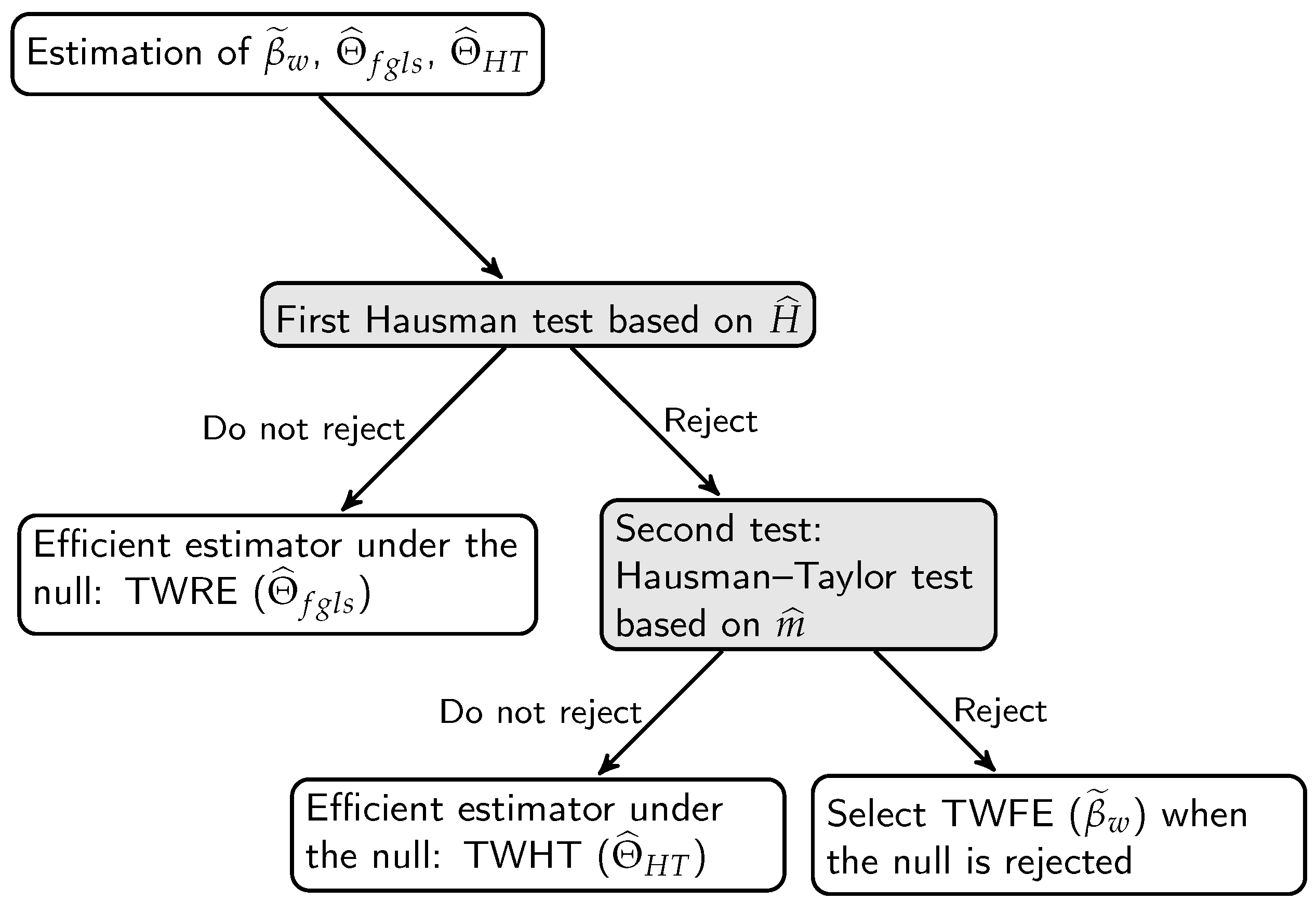
1985) and selects the two-way RE if the null hypothesis is not rejected. It then selects the two-way HT if it passes a second Hausman test based on two-way FE versus two-way HT. If this is rejected, the pretest selects the two-way FE estimator.2
In empirical applications, the two tests should be used successively, as shown in Figure 1. After calculating the TWFE ( β ˜ w ), TWRE ( Θ ^ f g l s ) and TWHT ( Θ ^ H T ) estimators, the first test is the Hausman test defined by H ^ = q ^ v a r ( β ˜ w ) v a r ( β ^ f g l s ) 1 q ^ , where q ^ = β ^ f g l s β ˜ w , and β ^ f g l s is a subset of Θ ^ f g l s . Under H 0 (none of the individual effects or time effects are correlated with the regressors), H ^ χ k 2 , and one chooses the efficient estimator TWRE. If this test is rejected, we use the over-identification test (called the Hausman–Taylor test in Figure 1) obtained by computing m ^ = q ^ v a r ( β ˜ w ) v a r ( β ^ H T ) q ^ , where q ^ = β ^ H T β ˜ w , with β ^ H T representing a subset of Θ ^ H T , and ⊖ is the symbol of the generalized inverse. Under H 0 , m ^ χ l 2 with l = 2 k 1 g 2 h 2 , and the efficient estimator TWHT is chosen. If the second test is rejected, the TWFE estimator is selected.
The pretest estimator may be written as
Θ ^ p r e = I ( 0 , c 1 ) ( H ^ ) Θ ^ f g l s + I [ c 1 , ) ( H ^ ) × I ( 0 , c 2 ) ( m ^ ) Θ ^ H T + I [ c 2 , ) ( m ^ ) β ˜ w ,
where I ( 0 , c 1 ) ( H ^ ) and I [ c 1 , ) ( H ^ ) are indicator functions that take the values I ( 0 , c 1 ) ( H ^ ) = 1 and I [ c 1 , ) ( H ^ ) = 0 if H ^ in the first Hausman test falls within the interval 0 and c 1 where c 1 is the 5% critical value for the χ k 2 statistics. This also means that I ( 0 , c 1 ) ( H ^ ) = 0 and I [ c 1 , ) ( H ^ ) = 1 when H ^ > c 1 . Likewise, I ( 0 , c 2 ) ( m ^ ) and I [ c 2 , ) ( m ^ ) are indicator functions that take the values I ( 0 , c 2 ) ( m ^ ) = 1 and I [ c 2 , ) ( m ^ ) = 0 if m ^ in the second Hausman–Taylor test falls within the interval 0 and c 2 where c 2 is the 5% critical value for the χ l 2 statistics. This also means that I ( 0 , c 2 ) ( m ^ ) = 0 and I [ c 2 , ) ( m ^ ) = 1 when m ^ > c 2 . It is clear from (3) that the pretest estimator is a function of the data, the hypothesis and the significance level of the two Hausman tests. As (3) is the sum of three parts, all three composed of products of non-independent random variables, and as underlined by Judge et al. (1978, 1988) and Giles and Giles (1993), to mention a few, the specification of the pretest estimator highlights the difficulty of deriving its sampling properties. And the choice of the significance level (here, 5%) of the χ 2 tests has a crucial role to play both in determining the proportion of use of each estimator and in determining the sampling performance of the pretest estimator.

3. Monte Carlo Results

Following Baltagi et al. (2003), we generalize the Monte Carlo design from the one-way to the two-way model:
y i t = α + X 1 , i t β 1 + X 2 , i t β 2 + γ 1 Z 1 i + γ 2 Z 2 i + δ 1 W 1 t + δ 2 W 2 t + μ i + λ t + ν i t
where X 1 , i t = [ X 11 , i t , X 12 , i t ] , β 1 = [ β 11 , β 12 ] . X 1 , i t is ( 1 × k 1 ) (here, k 1 = 2 ) . Z 2 i is ( 1 × g 2 ) (here, g 2 = 1 ) . Z 1 i and Z 2 i are the time-invariant variables described below. W 1 t and W 2 t are the individual-invariant variables described below.
In our experiments, we set α = 5 , β 1 = β 2 = γ 1 = γ 2 = δ 2 = 1 , μ i I I N ( 0 , σ μ 2 ) , λ t I I N ( 0 , σ λ 2 ) and ν i t I I N ( 0 , σ ν 2 ) independent of each other. The total variance across experiments is fixed at σ 2 = σ μ 2 + σ λ 2 + σ ν 2 = 3 . The proportion of variance due to individual effects ρ 1 = σ μ 2 / σ 2 as well as the proportion of variance due to time effects ρ 2 = σ λ 2 / σ 2 is varied over the set (0.1, 0.2, 0.4, 0.6, 0.8) such that ( 1 ρ 1 ρ 2 ) is always positive. We let ρ 3 = σ ν 2 / σ 2 = 0.1 , i.e., σ ν 2 = 0.3 . Then, ( ρ 1 , ρ 2 ) = ( ( 0.1 , 0.8 ) , ( 0.2 , 0.7 ) , ( 0.4 , 0.5 ) , ( 0.6 , 0.3 ) , ( 0.8 , 0.1 ) ) , to which we add the particular case ( ρ 1 , ρ 2 ) = ( 0 , 0 ) with σ ν 2 = σ 2 = 3 . The ( N , T ) values considered are ( 300 , 100 ) , ( 200 , 100 ) and ( 300 , 200 ) . The number of replications is 1000.
The X 1 variables are generated following Nerlove (1971). For these series, the ratios of the between-individual (Bxx), between-time (Cxx) and the within-individual–time (Wxx) variabilities relative to the total variability are roughly 71 % , 23 % and 6 % . Maddala and Mount (1973, p. 326) warned that for the two-way model, Wxx has to be small with respect to Bxx and Cxx; otherwise, the random-effects GLS would be equivalent to the fixed effects model, and the errors in the estimation of the variance components would not be of much consequence for estimating the slope coefficients. The X 1 , i t variables are not correlated with μ i and λ t , and are generated as follows:
X 11 , i t = 0.5 X 11 , i , t 1 + φ i + ϕ t + ζ i t X 12 , i , t = 0.5 X 12 , i , t 1 + ϑ i + τ t + ξ i t
where φ i , ϑ i t , ϕ t and τ t are uniform on [ 4 , 4 ] , ζ i t and ξ i t are uniform on [ 2 , 2 ] , and Z 1 i and W 1 t are uniform on [ 3 , 3 ] .
We focus on the following two designs:
Case 1—A two-way Hausman–Taylor world, where X 2 is correlated with μ i and λ t by design, and Z 2 i is correlated with μ i as well as X 11 , i t , X 12 , i t , X 2 , i t . Also, W 2 t is correlated with λ t as well as X 11 , i t , X 12 , i t , X 2 , i t .
X 2 , i t = 0.5 X 2 , i , t 1 + μ i + λ t + ϑ i t Z 2 i = μ i + φ i + ϑ i + χ i W 2 t = λ t + ϕ t + τ t + ψ t
In the above equations, χ i and ψ t are uniform on [ 4 , 4 ] , and ϑ i t is uniform on [ 2 , 2 ] . Z 2 i is correlated with X 11 , i t by the common term φ i , with X 12 , i , t by the common term ϑ i and with X 2 , i t by the common term μ i . W 2 t is correlated with X 11 , i t by the common term ϕ t , with X 12 , i , t by the common term τ t and with X 2 , i t by the common term λ t .
Case 2—A two-way random-effects world, where Z 2 i and W 2 t are not correlated with μ i and λ t , but are still correlated with X 11 , i t and X 12 , i t :
X 2 , i t = 0.5 X 2 , i , t 1 + κ i + ϱ t + ϑ i t Z 2 i = φ i + ϑ i + χ i W 2 t = ϕ t + τ t + ψ t
where κ i and ϱ t are uniform on [ 4 , 4 ] and where X 2 , i t is not correlated with μ i and λ t .
Table 1 shows the choice of the pretest estimator for various values of ( ρ 1 , ρ 2 ) in a Hausman–Taylor-type world when N = 300 and T = 100 . For example, when ( ρ 1 , ρ 2 ) = ( 0 , 0 ) , out of 1000 replications, the pretest estimator chose the RE estimator in 946 replications, the HT estimator in 24 replications and the FE estimator in 30 replications. For ( ρ 1 , ρ 2 ) ( 0 , 0 ) , almost all replications chose the HT estimator. None selected RE, and between 9 and 14 replications selected FE. Note that as we vary ( ρ 1 , ρ 2 ) , not only does the proportion of the total variance due to the random individual and time effects vary, but so does the extent of correlation between the regressors and the individual and time effects. For example, when ( ρ 1 , ρ 2 ) = ( 0.2 , 0.7 ) , the mean correlation between X 2 , i t and μ i is 0.59. This rises to 0.84 when ( ρ 1 , ρ 2 ) = ( 0.6 , 0.3 ) . In contrast, the mean correlation between X 2 , i t and λ t drops from 0.54 to 0.29 for these two cases. The mean correlation between Z 2 i and μ i is 0.19 and 0.32, and the mean correlation between W 2 t and λ t is 0.34 and 0.23 for these two cases. We focus on the coefficients of the endogenous regressors X 2 , Z 2 and W 2 , i.e., β 2 , γ 2 and δ 2 . The results of the other coefficients are available upon request from the authors. Table 1 reports the bias and RMSE (in %). When ( ρ 1 , ρ 2 ) = ( 0 , 0 ) , OLS performs well in terms of bias and RMSE for all coefficients. When ( ρ 1 , ρ 2 ) ( 0 , 0 ) , HT, pretest and FE are the best in terms of RMSE for β 2 , with HT and pretest performing the best for γ 2 and δ 2 . Table 1 also reports the frequency of rejections in 1000 replications for β 2 = 1 , γ 2 = 1 and δ 2 = 1 . This is assessed at the 5 % significance level. Since the null hypothesis is always true, this represents the empirical size of the test. As expected, OLS performs badly, rejecting the null hypothesis when true in 99 to 100 percent of the cases, when ( ρ 1 , ρ 2 ) ( 0 , 0 ) . The same is true for the RE estimator since endogeneity is present. On the other hand, HT performs well, giving a size close to the 5% level. FE performs well for β 2 , but it cannot estimate γ 2 and δ 2 . The pretest performs well, with a size between 5% and 6% for β 2 and γ 2 and between 5% and 7% for δ 2 .
Table 2 shows the choice of the pretest estimator for various values of ( ρ 1 , ρ 2 ) in a random effects-type world when N = 300 and T = 100 . For example, when ( ρ 1 , ρ 2 ) = ( 0.4 , 0.5 ) out of 1000 replications, the pretest estimator is an RE estimator in 951 replications and an HT estimator in 49 replications. Now, there is no correlation between the regressors and the random individual and time effects. Table 2 also reports the bias and RMSE (in %) for β 2 , γ 2 and δ 2 . When ( ρ 1 , ρ 2 ) = ( 0 , 0 ) , RE and OLS perform the best in terms of RMSE for all coefficients. The pretest is a distant third, while HT and the fixed-effects model perform poorly. When ( ρ 1 , ρ 2 ) ( 0 , 0 ) , in terms of RMSE, OLS performs poorly for all coefficients. RE is best, followed by the pretest and FE (only for β 2 ), and then, HT. For the frequency of rejections in 1000 replications for β 2 = 1 , γ 2 = 1 and δ 2 = 1 in an RE world, OLS is the only estimator that performs badly, rejecting the null hypothesis when true in a large percentage of cases, especially when ( ρ 1 ρ 2 ) are large. This is as large as 84% for β 2 , 81% for γ 2 and 88% for δ 2 .
Table 3 and Table 4 consider the two-way Hausman and Taylor world and two-way RE world for N = 200 and T = 100 , so that N / T = 2 , rather than 3 in the case of Table 1 and Table 2. Comparing Table 3 and Table 4 to Table 1 and Table 2, respectively, T remains fixed at 100, while N decreases from 300 to 200. Table 5 and Table 6 fix N at 300 and double T from 100 to 200. By and large, similar rankings in terms of RMSE occur as described in Table 1 and Table 2 but with different magnitudes.
As expected, holding T fixed at 100 and increasing N from 200 to 300, the RMSE of β 2 decreases for both the HT and RE worlds. In Table 3, the RMSE of the HT estimator of β 2 is of the order 0.296 to 0.300 for ( ρ 1 , ρ 2 ) ( 0 , 0 ) . This magnitude drops to the order 0.234 to 0.235 in Table 1 as N increases from 200 to 300, holding T fixed at 100. This RMSE range drops even further to ( 0.171 , 0.172 ) in Table 5 for N = 300 and T = 200 , i.e., increasing both N and T. A similar decline in RMSE occurs for γ 2 for the HT estimator. The RMSE range is ( 1.037 , 2.817 ) in Table 1 ( N = 300 , T = 100 ), compared to ( 1.272 , 3.414 ) in Table 3 ( N = 200 , T = 100 ) and ( 1.004 , 2.792 ) in Table 5 ( N = 300 , T = 200 ).
Similarly, for the RE estimator, the RMSE range for β 2 decreases from ( 0.277 , 0.290 ) in Table 4 (for N = 200 , T = 100 ) to ( 0.219 , 0.227 ) in Table 2 (for N = 300 , T = 100 ), and decreases further to ( 0.165 , 0.168 ) in Table 6 (for N = 300 , T = 200 ). A similar decline in the RMSE happens for γ 2 for the RE estimator. The RMSE range is ( 0.834 , 2.279 ) in Table 2 ( N = 300 , T = 100 ), compared to ( 0.983 , 2.669 ) in Table 4 ( N = 200 , T = 100 ), and ( 0.824 , 2.297 ) in Table 6 ( N = 300 , T = 200 ). For δ 2 , the RMSE performance improves as the N / T ratio declines. For the HT estimator, it is ( 2.053 , 5.819 ) for Table 1  ( N / T = 3 ) and drops to ( 2.025 , 5.680 ) for Table 3  ( N / T = 2 ) and ( 1.386 , 3.918 ) for Table 5  ( N / T = 1.5 ) . For the RE estimator, it is ( 1.426 , 4.019 ) for Table 2  ( N / T = 3 ) and drops to ( 1.405 , 3.935 ) for Table 4  ( N / T = 2 ) and ( 0.976 , 2.749 ) for Table 6  ( N / T = 1.5 ) .3
In summary, as in the one-way panel model, the OLS standard errors are biased and yield misleading inferences under both the two-way RE and HT worlds. RE, FE, HT and pretest yield the required 5% size under both designs for all values of ( ρ 1 , ρ 2 ) . As expected, the RE estimator yields correct inference under a two-way RE world, but leads to misleading inference under a two-way HT world. In terms of bias, RMSE and inference, the pretest estimator is a viable alternative to two-way FE, RE and HT and should be considered in empirical panel applications.

Author Contributions

The authors contributed equally to this work with regard to conceptualization, methodology, software, validation, formal analysis, investigation, resources, writing—original draft preparation, writing—review and editing, visualization, supervision and project administration. All authors have read and agreed to the published version of the manuscript.

Funding

This research received no external funding.

Institutional Review Board Statement

Not applicable.

Informed Consent Statement

Not applicable.

Data Availability Statement

Data sharing is not applicable because the article describes entirely theoretical research.

Acknowledgments

We would like to thank the editor and two anonymous referees for their valuable comments and suggestions.

Conflicts of Interest

The authors declare no conflicts of interest.

Notes

1
For an extension of the one-way Hausman and Taylor model to multidimensional panels, see Balazsi et al. (2017).
2
With large T panels, one may be concerned with serial correlation in the disturbances, and the Hausman and Taylor two-way estimator has to be modified to deal with this serial correlation.
3
These results corroborate assumptions 1 and 2 and theorem 2 of Wyhowski (1994) and in particular the important role of the constraint of a bounded N / T for asymptotic distributions. We also performed some robustness checks for alternative ( N , T ) combinations and alternative data generation processes for the exogenous and endogenous regressors.

References

  1. Balazsi, Laszlo, Maurice J. G. Bun, Felix Chan, and Mark N. Harris. 2017. Models with endogenous regressors, Chapter 3. In The Econometrics of Multi-Dimensional Panels. Advanced Studies in Theoretical and Applied Econometrics. Edited by Laszlo Matyas. Cham: Springer, vol. 50, pp. 71–100. [Google Scholar]
  2. Baltagi, Badi H. 2023a. The Two-way Mundlak Estimator. Econometric Reviews 42: 240–46. [Google Scholar] [CrossRef]
  3. Baltagi, Badi H. 2023b. The Two-way Hausman and Taylor Estimator. Economics Letters 228: 111159. [Google Scholar] [CrossRef]
  4. Baltagi, Badi H., Georges Bresson, and Alain Pirotte. 2003. Fixed effects, random effects or Hausman-Taylor? A pretest estimator. Economics Letters 79: 361–69. [Google Scholar] [CrossRef]
  5. Cornwell, Christopher, and Peter Rupert. 1988. Efficient estimation with panel data: An empirical comparison of instrumental variables estimators. Journal of Applied Econometrics 3: 149–55. [Google Scholar] [CrossRef]
  6. Egger, Peter, and Michael Pfaffermayr. 2004. Distance, trade and FDI: A Hausman-Taylor SUR approach. Journal of Applied Econometrics 19: 227–46. [Google Scholar] [CrossRef]
  7. Fuller, Wayne A., and George E. Battese. 1974. Estimation of linear models with cross-error structure. Journal of Econometrics 2: 67–78. [Google Scholar] [CrossRef]
  8. Giles, Judith A., and David E.A. Giles. 1993. Pre-test estimation and testing in econometrics: Recent developments. Journal of Economic Surveys 7: 145–97. [Google Scholar] [CrossRef]
  9. Glick, Reuven, and Andrew K. Rose. 2002. Does a currency union affect trade? The time series evidence. European Economic Review 46: 1125–51. [Google Scholar] [CrossRef]
  10. Hausman, Jerry A. 1978. Specification tests in econometrics. Econometrica 46: 1251–71. [Google Scholar] [CrossRef]
  11. Hausman, Jerry A., and William E. Taylor. 1981. Panel data and unobservable individual effects. Econometrica 49: 1377–98. [Google Scholar] [CrossRef]
  12. Judge, George G., and Mary E. Bock. 1978. The Statistical Implications of Pre-Test and Stein-Rule Estimators in Econometrics. Amsterdam: Elsevier. [Google Scholar]
  13. Judge, George G., R. Carter Hill, William E. Griffiths, Helmut Lutkepohl, and Tsoung-Chao Lee. 1988. Introduction to the Theory and Practice of Econometrics. New York: John Wiley & Sons. [Google Scholar]
  14. Kang, Suk. 1985. A note on the equivalence of specification tests in the two-factor multivariate variance components model. Journal of Econometrics 28: 193–203. [Google Scholar] [CrossRef]
  15. Maddala, Gangadharrao S., and Timothy D. Mount. 1973. A comparative study of alternative estimators for variance components models used in econometric applications. Journal of the American Statistical Association 68: 324–28. [Google Scholar] [CrossRef]
  16. Moulton, Brent R. 1986. Random group effects and the precision of regression estimates. Journal of Econometrics 32: 385–97. [Google Scholar] [CrossRef]
  17. Mundlak, Yair. 1978. On the pooling of time series and cross-section data. Econometrica 46: 69–85. [Google Scholar] [CrossRef]
  18. Nerlove, Marc. 1971. Further evidence on the estimation of dynamic economic relations from a time series of cross sections. Econometrica 39: 359–82. [Google Scholar] [CrossRef]
  19. Owusu-Gyapong, Anthony. 1986. Alternative estimating techniques for panel data on strike activity. Review of Economics and Statistics 68: 526–31. [Google Scholar] [CrossRef]
  20. Serlenga, Laura, and Yongcheol Shin. 2007. Gravity models of intra-EU trade: Application of the CCEP-HT estimation in heterogeneous panels with unobserved common time-specific factors. Journal of Applied Econometrics 22: 361–81. [Google Scholar] [CrossRef]
  21. Wooldridge, Jeffrey M. 2021. Two-Way Fixed Effects, the Two-Way Mundlak Regression, and Difference-in-Differences Estimator. Available online: https://www.researchgate.net/publication/353938385_Two-Way_Fixed_Effects_the_Two-Way_Mundlak_Regression_and_Difference-in-Differences_Estimators (accessed on 4 December 2023).
  22. Wyhowski, Donald J. 1994. Estimation of a panel data model in the presence of correlation between regressors and a two-way error component. Econometric Theory 10: 130–39. [Google Scholar] [CrossRef]
Figure 1. Pretest estimator.
Econometrics 12 00009 g001
Table 1. Hausman–Taylor world. Count, bias, RMSE, 5 % size, N = 300 , T = 100 , 1000 replications. 
Count Within β 2
( ρ 1 , ρ 2 ) REHTFE biasrmsesize
1 ( 0.0 , 0.0 ) 9462430 0.0320.7555
2 ( 0.1 , 0.8 ) 1097911 0.0040.2355
3 ( 0.2 , 0.7 ) 09919 0.0040.2355
4 ( 0.4 , 0.5 ) 098614 0.0040.2355
5 ( 0.6 , 0.3 ) 098812 0.0040.2345
6 ( 0.8 , 0.1 ) 098911 0.0040.2345
OLS RE
β 2 γ 2 δ 2 β 2 γ 2 δ 2
biasrmsesizebiasrmsesizebiasrmsesize biasrmsesizebiasrmsesizebiasrmsesize
10.0320.75450.0070.3595−;0.0050.2885 0.0320.75450.0070.3594−;0.0050.2884
244.92644.9531004.1664.2761008.9969.224100 19.41019.4231002.8322.90810011.23811.497100
344.37044.3871004.1474.2491008.1948.421100 27.40827.4191004.0224.0761009.4959.73499
443.41143.4181004.2244.3061006.4576.687100 34.56134.5691005.1075.1421007.0287.25394
542.51342.5161004.4264.4821004.5464.770100 37.85737.8631005.6235.6501004.9295.13586
641.59041.5921004.7454.7761002.4452.61099 39.75239.7571005.9225.9461002.8783.01583
Hausman-Taylor Pretest
β 2 γ 2 δ 2 β 2 γ 2 δ 2
biasrmsesizebiasrmsesizebiasrmsesize biasrmsesizebiasrmsesizebiasrmsesize
10.0320.7565−;0.0481.1024−;0.0250.8014 0.0320.75550.0030.4945−;0.0090.3715
20.0060.23550.0071.0374−;0.0385.8196 0.1821.75260.0501.09650.0485.9247
30.0060.23550.0121.4325−;0.0365.4386 0.0060.23550.0151.4325−;0.0605.4436
40.0060.23550.0192.0025−;0.0304.5876 0.0060.23550.0202.0115−;0.0484.5936
50.0060.23450.0252.4446−;0.0233.5486 0.0060.23450.0402.4446−;0.0203.5526
60.0060.23450.0292.8175−;0.0142.0536 0.0060.23450.0452.8105−;0.0202.0576
bias × 10 2 , rmse × 10 2 .
Table 2. Random-effects world. Count, bias, rmse, 5 % size, N = 300 , T = 100 , 1000 replications. 
Count Within β 2
( ρ 1 , ρ 2 ) REHTFE biasrmsesize
1 ( 0.0 , 0.0 ) 9492724 0.0250.7375
2 ( 0.1 , 0.8 ) 954460 0.0050.2294
3 ( 0.2 , 0.7 ) 951481 0.0050.2294
4 ( 0.4 , 0.5 ) 951490 0.0050.2294
5 ( 0.6 , 0.3 ) 948520 0.0050.2294
6 ( 0.8 , 0.1 ) 944560 0.0050.2294
OLS RE
β 2 γ 2 δ 2 β 2 γ 2 δ 2
biasrmsesizebiasrmsesizebiasrmsesize biasrmsesizebiasrmsesizebiasrmsesize
1−;0.0080.18240.0080.3605−;0.0050.2885 −;0.0070.18240.0070.3604−;0.0050.2884
2−;0.0441.46882−;0.0142.40378−;0.0484.14088 0.0040.2194−;0.0030.8345−;0.0324.0196
3−;0.0451.47983−;0.0192.48978−;0.0483.89186 0.0040.2244−;0.0021.1586−;0.0303.7606
4−;0.0451.49482−;0.0272.65179−;0.0463.33485 0.0040.22740.0001.6205−;0.0253.1786
5−;0.0421.50584−;0.0332.80480−;0.0412.66082 0.0040.22840.0011.9776−;0.0192.4636
6−;0.0361.51084−;0.0382.94981−;0.0331.73376 0.0040.22740.0022.2795−;0.0101.4266
Hausman-Taylor Pretest
β 2 γ 2 δ 2 β 2 γ 2 δ 2
biasrmsesizebiasrmsesizebiasrmsesize biasrmsesizebiasrmsesizebiasrmsesize
10.0210.7184−;0.0491.1014−;0.0260.8064 0.0040.33160.0070.5035−;0.0060.3755
20.0050.22940.0051.0374−;0.0435.7426 0.0050.2204−;0.0070.8786−;0.0894.1326
30.0050.22940.0101.4335−;0.0415.3726 0.0040.2244−;0.0081.2166−;0.0613.8796
40.0050.22940.0172.0045−;0.0354.5436 0.0040.2264−;0.0081.6986−;0.0623.3046
50.0050.22940.0232.4466−;0.0273.5246 0.0040.2274−;0.0072.0656−;0.0532.5706
60.0050.22940.0272.8206−;0.0162.0465 0.0040.2274−;0.0162.3636−;0.0091.5186
bias × 10 2 , rmse × 10 2 .
Table 3. Hausman–Taylor world. Count, bias, rmse, 5 % size, N = 200 , T = 100 , 1000 replications. 
Count Within β 2
( ρ 1 , ρ 2 ) REHTFE biasrmsesize
1 ( 0.0 , 0.0 ) 9631126 0.0310.9536
2 ( 0.1 , 0.8 ) 3894715 0.0310.2995
3 ( 0.2 , 0.7 ) 098614 0.0310.2995
4 ( 0.4 , 0.5 ) 098713 0.0310.2985
5 ( 0.6 , 0.3 ) 09955 0.0310.2965
6 ( 0.8 , 0.1 ) 098812 0.0310.2955
OLS RE
β 2 γ 2 δ 2 β 2 γ 2 δ 2
biasrmsesizebiasrmsesizebiasrmsesize biasrmsesizebiasrmsesizebiasrmsesize
10.0290.95060.0170.4364−;0.0090.3484 0.0300.95060.0180.4373−;0.0090.3484
244.92844.9561004.2004.3211009.0939.311100 19.34519.3621002.8492.96010011.36911.612100
344.36144.3791004.1774.2901008.2898.507100 27.31327.3281004.0464.1231009.6199.84699
443.38943.3971004.2494.3391006.5456.764100 34.46534.4761005.1385.1891007.1347.35096
542.48242.4851004.4464.5111004.6194.833100 37.77137.7791005.6585.6971005.0145.21487
641.54941.5511004.7634.8021002.4922.65499 39.67639.6821005.9555.9881002.9313.06981
Hausman-Taylor Pretest
β 2 γ 2 δ 2 β 2 γ 2 δ 2
biasrmsesizebiasrmsesizebiasrmsesize biasrmsesizebiasrmsesizebiasrmsesize
10.0310.95360.0591.36050.0250.9875 0.0300.95060.0310.5234−;0.0010.3994
20.0330.3005−;0.0501.27250.0825.6806 0.7123.49190.1311.43190.5256.07010
30.0340.2995−;0.0731.74550.0785.3116 0.0330.2995−;0.0721.74950.0645.3256
40.0340.2985−;0.1042.43050.0704.4886 0.0330.2985−;0.1062.43250.0804.4876
50.0330.2975−;0.1292.96260.0583.4806 0.0330.2975−;0.1252.96260.0563.4856
60.0330.2965−;0.1493.41450.0372.0255 0.0330.2965−;0.1383.42450.0332.0285
bias × 10 2 , rmse × 10 2 .
Table 4. Random-effects world. Count, bias, rmse, 5 % size, N = 200 , T = 100 , 1000 replications. 
Count Within β 2
( ρ 1 , ρ 2 ) REHTFE biasrmsesize
1 ( 0.0 , 0.0 ) 9462628 0.0280.9265
2 ( 0.1 , 0.8 ) 935641 0.0260.2955
3 ( 0.2 , 0.7 ) 937621 0.0260.2955
4 ( 0.4 , 0.5 ) 940582 0.0260.2955
5 ( 0.6 , 0.3 ) 941590 0.0260.2955
6 ( 0.8 , 0.1 ) 948502 0.0260.2955
OLS RE
β 2 γ 2 δ 2 β 2 γ 2 δ 2
biasrmsesizebiasrmsesizebiasrmsesize biasrmsesizebiasrmsesizebiasrmsesize
10.0070.22850.0170.4364−;0.0090.3474 0.0080.22850.0170.4373−;0.0090.3484
20.0641.533760.0022.582740.1314.13188 0.0260.2774−;0.0250.98350.1073.9356
30.0691.574770.0032.734760.1313.89388 0.0270.2855−;0.0371.36040.1003.6826
40.0731.652790.0053.013780.1253.36386 0.0270.2895−;0.0531.90050.0843.1145
50.0731.725790.0063.266800.1132.72483 0.0280.2905−;0.0662.31750.0652.4165
60.0671.793780.0073.499810.0901.86774 0.0280.2905−;0.0762.66950.0381.4055
Hausman-Taylor Pretest
β 2 γ 2 δ 2 β 2 γ 2 δ 2
biasrmsesizebiasrmsesizebiasrmsesize biasrmsesizebiasrmsesizebiasrmsesize
10.0280.89450.0581.36350.0210.9955 −;0.0060.46970.0260.6114−;0.0030.4634
20.0260.2955−;0.0531.27050.1165.6705 0.0260.2825−;0.0391.03550.0913.9966
30.0260.2955−;0.0751.74250.1085.3055 0.0270.2875−;0.0591.42140.0613.7556
40.0260.2955−;0.1072.42260.0914.4875 0.0280.2905−;0.0751.97050.0693.2226
50.0270.2955−;0.1322.94950.0703.4826 0.0270.2915−;0.0702.39450.0742.5146
60.0270.2955−;0.1533.39650.0402.0285 0.0270.2905−;0.0812.71550.0451.4996
bias × 10 2 , rmse × 10 2 .
Table 5. Hausman–Taylor world. Count, bias, rmse, 5 % size, N = 300 , T = 100 , 1000 replications. 
Count Within β 2
( ρ 1 , ρ 2 ) REHTFE biasrmsesize
1 ( 0.0 , 0.0 ) 9591922 0.0120.5274
2 ( 0.1 , 0.8 ) 79858 0.0000.1725
3 ( 0.2 , 0.7 ) 09937 0.0000.1725
4 ( 0.4 , 0.5 ) 098911 0.0000.1725
5 ( 0.6 , 0.3 ) 098515 0.0000.1715
6 ( 0.8 , 0.1 ) 098020 0.0000.1714
OLS RE
β 2 γ 2 δ 2 β 2 γ 2 δ 2
biasrmsesizebiasrmsesizebiasrmsesize biasrmsesizebiasrmsesizebiasrmsesize
10.0120.52540.0000.2616−;0.0090.2086 0.0120.52540.0000.2616−;0.0090.2076
244.74844.7611004.2184.2791009.0769.181100 19.28519.2971002.8242.90410011.34811.462100
344.19744.2051004.1864.2421008.2778.382100 27.25827.2691004.0174.0731009.5979.705100
443.24543.2481004.2384.2841006.5396.646100 34.40234.4091005.0985.1341007.1167.220100
542.34942.3511004.4174.4521004.6164.721100 37.70037.7061005.6065.6341005.0005.097100
641.42441.4251004.7174.7401002.4872.567100 39.60239.6061005.8955.9181002.9222.98899
Hausman-Taylor Pretest
β 2 γ 2 δ 2 β 2 γ 2 δ 2
biasrmsesizebiasrmsesizebiasrmsesize biasrmsesizebiasrmsesizebiasrmsesize
10.0120.5274−;0.0310.7656−;0.0260.5475 0.0120.5254−;0.0060.3667−;0.0120.2707
20.0010.1725−;0.0491.00450.0773.9185 0.1211.4435−;0.0271.04460.1364.0535
30.0010.1725−;0.0621.40450.0723.6635 0.0010.1725−;0.0651.40650.0653.6685
40.0010.1724−;0.0801.97650.0613.0944 0.0010.1724−;0.0751.97950.0563.0934
50.0010.1714−;0.0942.41850.0472.3955 0.0010.1714−;0.0932.42050.0572.3975
60.0010.1714−;0.1052.79250.0241.3864 0.0010.1714−;0.0942.78550.0281.3914
bias × 10 2 , rmse × 10 2 .
Table 6. Random-effects world. Count, bias, rmse, 5 % size, N = 300 , T = 100 , 1000 replications. 
Count Within β 2
( ρ 1 , ρ 2 ) REHTFE biasrmsesize
1 ( 0.0 , 0.0 ) 9452431 0.0140.5194
2 ( 0.1 , 0.8 ) 949492 −;0.0010.1694
3 ( 0.2 , 0.7 ) 947512 −;0.0010.1694
4 ( 0.4 , 0.5 ) 955450 −;0.0010.1694
5 ( 0.6 , 0.3 ) 959410 −;0.0010.1694
6 ( 0.8 , 0.1 ) 960391 −;0.0010.1694
OLS RE
β 2 γ 2 δ 2 β 2 γ 2 δ 2
biasrmsesizebiasrmsesizebiasrmsesize biasrmsesizebiasrmsesizebiasrmsesize
1−;0.0030.13340.0010.2616−;0.0090.2076 −;0.0040.13340.0010.2616−;0.0090.2075
2−;0.0391.10282−;0.0061.918800.1502.88088 −;0.0020.1654−;0.0450.82440.1302.7496
3−;0.0451.16183−;0.0252.114820.1392.71188 −;0.0020.1674−;0.0591.15550.1222.5726
4−;0.0511.26984−;0.0532.453830.1162.34288 −;0.0020.1685−;0.0791.62750.1032.1746
5−;0.0551.36686−;0.0772.746850.0881.90785 −;0.0020.1684−;0.0941.99050.0791.6856
6−;0.0561.45386−;0.1013.006880.0481.34276 −;0.0020.1685−;0.1072.29750.0450.9766
6
Hausman-Taylor Pretest
β 2 γ 2 δ 2 β 2 γ 2 δ 2
biasrmsesizebiasrmsesizebiasrmsesize biasrmsesizebiasrmsesizebiasrmsesize
10.0150.5114−;0.0290.7655−;0.0260.5485 0.0060.2556−;0.0010.3587−;0.0100.2656
2−;0.0010.1694−;0.0491.00250.0923.9065 −;0.0020.1654−;0.0420.84850.1182.8035
3−;0.0010.1694−;0.0621.39950.0853.6545 −;0.0010.1674−;0.0561.18750.1032.6135
4−;0.0010.1694−;0.0811.96650.0713.0895 −;0.0010.1685−;0.0821.66950.0792.2395
5−;0.0010.1694−;0.0952.40350.0532.3944 −;0.0010.1694−;0.1072.03450.0621.7616
6−;0.0010.1694−;0.1062.77250.0261.3874 −;0.0020.1685−;0.1132.32850.0311.0306
bias × 10 2 , rmse × 10 2 .
Disclaimer/Publisher’s Note: The statements, opinions and data contained in all publications are solely those of the individual author(s) and contributor(s) and not of MDPI and/or the editor(s). MDPI and/or the editor(s) disclaim responsibility for any injury to people or property resulting from any ideas, methods, instructions or products referred to in the content.

