Article

Public Debt and Economic Growth: A Panel Kink Regression Latent Group Structures Approach †

1
Magyar Nemzeti Bank (Central Bank of Hungary), 1054 Budapest, Hungary
2
MNB Institute, John von Neumann University, 6000 Kecskemét, Hungary
3
Department of Economics and Finance, University of Guelph, Guelph, ON N1G 2W1, Canada
*
Author to whom correspondence should be addressed.
The views expressed here are the authors’ and not necessarily those of the Central Bank of Hungary.
Econometrics 2024, 12(1), 7; https://doi.org/10.3390/econometrics12010007
Submission received: 6 January 2024 / Revised: 10 February 2024 / Accepted: 28 February 2024 / Published: 5 March 2024

Abstract

:
This paper investigates the relationship between public debt and economic growth in the context of a panel kink regression with latent group structures. The proposed model allows us to explore the heterogeneous threshold effects of public debt on economic growth based on unknown group patterns. We propose a least squares estimator and demonstrate the consistency of estimating group structures. The finite sample performance of the proposed estimator is evaluated by simulations. Our findings reveal that the nonlinear relationship between public debt and economic growth is characterized by a heterogeneous threshold level, which varies among different groups, and highlight that the mixed results found in previous studies may stem from the assumption of a homogeneous threshold effect.
JEL Classification:
C23; C24; O40

1. Introduction

In recent years, particularly during the COVID-19 pandemic, many countries have seen a consistent rise in public debt. This trend has sparked concerns about its potential effects on sustained economic growth. According to the conventional view, rooted in the Ricardian Equivalence theory, the negative impacts of rising public debt could be offset by an equal increase in private savings. This suggests that the overall national savings would remain unchanged, thus not influencing growth (e.g., Barro 1974). Conversely, if Ricardian Equivalence is not applicable, another strand of the literature believes that increased public debt could negatively affect long-term economic growth (e.g., Blanchard 1985; Elmendorf and Gregory Mankiw 1999).
Recent studies have shifted towards exploring potential nonlinear dynamics within the debt–growth nexus, examining how accumulating debt might adversely affect economic growth, particularly when debt levels surpass certain thresholds. A seminal study by Reinhart and Rogoff (2010) posits that public debt begins to impede economic growth when the debt-to-GDP ratio exceeds 90%. Using threshold regression models, studies by Afonso and Jalles (2013); Caner et al. (2010); Cecchetti et al. (2011) identified varying thresholds of debt-to-GDP ratios, 85%, 77%, and 59%, respectively, at which public debt begins to harm economic growth. However, Kourtellos et al. (2013) were unable to confirm a significant threshold effect for public debt when adjusting for endogeneity concerns.
The above-mentioned studies provide mixed evidence about the nonlinear effects of public debt on economic growth and two main challenges emerge. Firstly, these findings are obtained under strong assumptions of homogeneity in threshold levels across different countries. Commonly, heterogeneity is modeled as a unit-specific, time-invariant fixed effect. For example, Chudik et al. (2017) examines a dynamic heterogeneous panel threshold model with cross-sectional dependent errors, yet this approach still assumes a uniform threshold level for all countries. Likewise, Eberhardt and Presbitero (2015) model the long-run relationship between public debt and growth as heterogeneous across countries. However, they introduce nonlinearities at the country level by using pre-determined thresholds. Employing the grouped fixed-effect estimator proposed by Bonhomme and Manresa (2015), Gómez-Puig et al. (2022) examine the heterogeneous link between public debt and economic growth by identifying the latent group patterns within fixed effects. Nevertheless, their research is limited to a linear panel model, neglecting potential nonlinear impacts. In short, the complexity of heterogeneous threshold modeling and the extensive data requirement may be reasons why few studies have concurrently addressed the two critical aspects—nonlinearity and heterogeneity—that are central to the debt–growth relationship. To identify heterogeneous threshold levels, there is a pressing need for applied researchers to develop a new model, that can balance the use of flexible methods for modeling unobserved heterogeneity with the development of parsimonious specifications that are feasible within the constraints of limited datasets. Secondly, conventional threshold regression models assume a discontinuous regression function at the true threshold level, which may not be suitable in this context. It is not intuitively expected to observe an abrupt jump in the economic growth rate when the public debt ratio increases marginally at the turning point. Chan and Tsay (1998) introduce a continuous threshold autoregressive model, which enables a piece-wise linear function of the threshold variable. Building on this, Hansen (2017) expands the framework by proposing tests for a threshold effect and inferring the regression parameters in a continuous threshold model with an unknown threshold parameter, termed the kink threshold regression (KTR) model. This model is also applied to re-examine the issue of public debt overhang, albeit under the assumption of a uniform threshold level. Motivated by previous work, we employ a panel kink threshold regression model with latent group structures to re-examine the debt–growth puzzle. Our contribution is twofold, encompassing both methodological and empirical approaches, and can be outlined as follows.
In terms of methodology, the proposed model extends the panel threshold regression model with latent group structures of Miao et al. (2020) by incorporating a continuous threshold effect. It is important to note that the theoretical distinction of the KTR model lies in its continuity property, setting it apart from the standard (discontinuous) threshold regression (TR) model. Firstly, the asymptotic distribution of the least squares estimator of the threshold in the KTR model and the TR model are quite different. In the KTR model, the estimator yields a normal distribution, whereas in the TR model, the estimator follows a two-sided Brownian motion with a diminishing threshold effect (see Hansen 2000), or a Poisson distribution under the fixed-threshold-effect assumption (see Chan 1993). Secondly, even though the KTR model can be perceived as a constrained TR model, Hidalgo et al. (2019) emphasizes that mistakenly estimating a KTR model within the TR framework of Hansen (2000) without considering the continuity of the true model results in an irregular Hessian matrix. This irregularity leads to the least squares estimator of the threshold parameter converging at a cube root-n convergence rate, slower than the root-n convergence rate observed for the KTR model, as demonstrated by Hansen (2017). All these references imply that the methodology outlined in Miao et al. (2020) cannot be directly applied to address the latent group structure problem in a KTR model and necessitates a conversion of our theoretical contribution. This model enables variations in threshold and slope coefficients across individuals through a group-based pattern within a continuous-threshold-effect framework, effectively addressing the previously mentioned two challenges. The proposed data-driven method aligns with other studies in panel latent group structures (e.g., Bonhomme and Manresa 2015; Su et al. 2016; Bonhomme et al. 2022), balancing the trade-off between the limited flexibility of homogeneity assumptions and the extensive data requirements of heterogeneity inherently. We present the estimation strategy and show the latent group structure can be estimated consistently with a probability that approaches 1. This extends theorem 3.1 from Miao et al. (2020) to the context of continuous threshold effects.
Empirically, using the dataset of Chudik et al. (2017), encompassing data from forty countries spanning from 1980 to 2010, the empirical results determine that the optimal number of groups is three and recover the group structures. For all countries, two groups benefit significantly from increasing public debt, up to a certain threshold, beyond which the significance diminishes. Within the subset of OECD countries, the group—made up of sixteen out of twenty-one OECD countries—exhibits an inverse U-shaped relationship between public debt and economic growth. The findings indicate the presence of a heterogeneous threshold effect, suggesting that any contradictory conclusions in the previous studies might stem from overlooking this heterogeneous impact on the way countries manage their debt obligations.
The rest of the paper is organized as follows. Section 2 describes the panel kink threshold regression model and the estimation strategy. Section 3 details the assumptions and establishes the consistency of the estimators for group membership. In Section 4, we evaluate the finite-sample performance of our model through Monte Carlo simulations. The empirical results of our study are presented in Section 5. Section 6 concludes the paper. Technical proofs are relegated to the Appendix A and Appendix B.

2. The Model and Estimates

This section presents the panel kink regression model in latent group structure and introduces the estimation procedure.

2.1. The Model

To explore the heterogeneous threshold effects of the public debt on economic growth, we consider the following panel kink threshold regression model with latent group structures,
y i t = α g i 0 0 + ρ g i 0 0 y i t 1 + β 1 , g i 0 0 d i , t 1 γ g i 0 0 I ( d i , t 1 γ g i 0 0 ) + β 2 , g i 0 0 d i , t 1 γ g i 0 0 I ( d i , t 1 > γ g i 0 0 ) + x i t β 3 , g i 0 0 + u i t ,
for i = 1 , , N , t = 1 , , T , where N denotes the number of cross-sectional units and T the number of time periods. The y i t variable represents the economic growth in country i in year t. The lagged dependent variable is included on the right-hand side to capture persistency in economic growth. The main variable of interest is the lagged value of the logarithm of the public debt-to-GDP ratio (multiplied by 100), denoted by d i t 1 . We deliberately choose the lagged public debt-to-GDP ratio as the threshold variable given the substantial evidence suggesting that contemporaneous public debt is endogenous (e.g., Frankel and Romer 1999; Panizza and Presbitero 2013).1 The term x i , t is a k × 1 vector, encompassing all remaining covariates.2 Following Miao et al. (2020), the model allows both the slope and kink coefficient parameters to be group-specific, where g i determines the group membership with g G { 1 , , G } and G is the number of groups. Thus, within the same group g, all members have the same coefficients ( α g i 0 , β 1 , g i 0 , β 2 , g i 0 , β 3 , g i 0 , ρ g i 0 , γ g i 0 ) . u i t is the random disturbance term, which is assumed to be serially uncorrelated over t. Let F N T , t be the smallest sigma field generated by { y i , t j , d i , t 1 j , x i , t j , u i , t j : j 0 } i = 1 N . We assume E ( u i t | F N T , t 1 ) = 0 for all i = 1 , , N and t = 1 , , T . Many previous models in the literature can be considered special cases of our model, as represented by Equation (1). For instance, if G = 1 is known a priori, all countries are categorized into the same group, and model (1) then becomes a pooled panel kink regression model, akin to the one proposed by Hansen (2017). Alternatively, if β 1 , g i 0 0 = β 2 , g i 0 0 , model (1) simplifies to a heterogeneous panel model with group patterns, as introduced by Bonhomme and Manresa (2015).

2.2. Estimation

Let D ( γ 1 , , γ G ) D G , G ( g 1 , , g N ) G N and Θ ( θ 1 , , θ G ) B G , where θ g ( α g , ρ g , β 1 , g , β 2 , g , β 3 , g ) B R 4 + k . We denote the true parameters as ( Θ 0 , D 0 , G 0 ) , where Θ 0 ( θ 1 0 , , θ G 0 ) , D 0 ( γ 1 0 , , γ G 0 ) , and G 0 ( g 1 0 , , g N 0 ) . Model (1) can be estimated as the following steps:
Denote χ i t ( γ g i ) = [ 1 , y i t 1 , d i , t 1 γ g i 0 0 I ( d i , t 1 γ g i 0 0 ) , d i , t 1 γ g i 0 0 I ( d i , t 1 > γ g i 0 0 ) , x i t ] . Given G , the least squares estimator of ( Θ , D , G ) is given by
( Θ ^ , D ^ , G ^ ) = argmin ( Θ , D , G ) B G × D G × G N Q N T ( Θ , D , G ) ,
where
Q N T ( Θ , D , G ) = 1 N T i = 1 N t = 1 T y i t χ i t ( γ g i ) θ g i 2 .
For any given D and group structure G, the slope coefficients θ g , g = 1 , , G , can be estimated by
θ ^ g ( D , G ) = i = 1 N t = 1 T I ( g i = g ) χ i t ( γ g ) χ i t ( γ g ) 1 i = 1 N t = 1 T I ( g i = g ) χ i t ( γ g ) y i t .
Then, we can estimate D and G as
( D ^ , G ^ ) = argmin ( D , G ) D G , G N Q N T Θ ^ ( D , G ) , D , G ,
where Θ ^ ( D , G ) = [ θ ^ 1 ( D , G ) , , θ ^ G ( D , G ) ] .
For addressing the optimization challenge outlined, we use the EM-type iterative algorithm (Algorithm 1) for exploring the ( D , G ) space, as proposed by Miao et al. (2020).
Algorithm 1: EM-type iterative algorithm
Initialize G ( 0 ) as a random starting point for the group structure G and set s = 0 .
Step 1 Given G ( s ) , compute the following:
D ( s ) = argmin D D G Q N T Θ ^ ( D , G ( s ) ) , D , G ( s ) .
Step 2 Given D ( s ) and G ( s ) , compute the slope coefficients for each group:
θ ^ g ( s ) = i = 1 N t = 1 T I ( g i ( s ) = g ) χ i t ( γ g ( s ) ) χ i t ( γ g ( s ) ) 1 i = 1 N t = 1 T I ( g i = g ) χ i t ( γ g ( s ) ) y i t .
Step 3 Compute the following for all i { 1 , , N } :
g i ( s + 1 ) = argmin g G t = 1 T y i t θ ^ g ( s ) χ i t ( γ g ( s ) ) 2 .
Step 4 Set s = s + 1 and continue repeating steps 1–3 until numerical convergence is achieved.

3. Asymptotic Results

In this section, the limiting distributions of the estimators for the group structure are discussed. Below, we list some regularity conditions used to derive the consistency of the group structure estimator.
Assumption 1.
(i) For each i = 1 , , N , t = 1 , , T , E ( u i t | F N T , t 1 ) = 0 , where F N T , t is the smallest sigma field generated by { y i , t j , d i , t 1 j , x i , t j , u i , t j : j 0 } i = 1 N .
(ii) Across i , ( y i t , d i , t 1 , x i t , u i t ) : t = 1 , , T are mutually independent of each other.
(iii) For all i, { w i t } = ( y i t , d i , t 1 , x i t , u i t ) , t 1 are strictly stationary mixing process with mixing coefficients α i ( t ) satisfying max 1 i N α i [ t ] C α ρ t for some constants C α > 0 & ρ ( 0 , 1 ) .
Assumption 2.
(i) For some ϵ > 0 and some constants C ϵ , max i , t E | y i t | 8 + ϵ C ϵ , max i , t E | d i t | 8 + ϵ C ϵ , max i , t E x i t 8 + ϵ C ϵ , and max i , t E | u i t | 8 + ϵ C ϵ .
(ii) The parameter spaces B and D are compact such that sup θ θ B C and D = [ γ ̲ , γ ¯ ] .
(iii) d i t has a density function f i t ( . ) and f i t ( γ ) is continuous over D and max i , t f i t ( γ ) c f < .
(iv) Let d i , t 1 ( γ ) = d i , t 1 γ I ( d i , t 1 γ ) and d i , t 1 + ( γ ) = d i , t 1 γ I ( d i , t 1 > γ ) . For some constants c > 0 , as ( N , T ) , we have
sup 1 i N sup | θ θ * | B sup | γ γ * | D { Pr [ t = 1 T θ χ i t ( γ ) θ * T χ i t ( γ * ) 2 c t = 1 T ( θ θ * ) χ i t ( γ * ) 2 + β 1 * d i , t 1 ( γ ) d i , t 1 ( γ * ) 2 + β 2 * d i , t 1 + ( γ ) d i , t 1 + ( γ * ) 2 ] } = o ( T 4 ) .
(v) Define
M N T ( g , g ˜ , G , D ) = 1 N T i = 1 N t = 1 T I ( g i 0 = g ) I ( g i = g ˜ ) χ i t ( g ˜ ) χ i t ( g ˜ ) .
There exists a constant c ̲ λ > 0 such that for all g G
P r inf ( G , D ) G N × D G max g ˜ G λ min [ M N T ( g , g ˜ , G , D ) ] > c ̲ λ 1 .
(vi) For all g , g ˜ G and g g ˜ , we have ( θ g 0 , γ g 0 ) ( θ g ˜ 0 , γ g ˜ 0 ) > C ̲ θ γ for some constants C ̲ θ γ > 0 .
(vii) For any g g ˜ and 1 i N , for some constants C ̲ g g ˜ > 0 , we have
max E ( θ g ˜ 0 θ g 0 ) χ i t ( γ g 0 ) 2 , | γ g ˜ 0 γ g 0 | 2 C ̲ g g ˜ , i C ̲ g g ˜ .
(viii) For all g G : lim N N g N = π g > 0 .
(ix) As ( N , T ) , N = O ( T 2 ) and T = O ( N 2 ) .
Assumption 1 is similar to assumptions A.1 (i)–(iii) of Miao et al. (2020) and assumptions A.2 (a)–(c) of Su and Chen (2013) and is standard in the literature. Assumption 1 (i) assumes the martingale difference sequence condition and Assumption 1 (ii) is the cross-sectional independence. Assumption 1 (iii) imposes the strong mixing condition.3
Assumptions 2 (i)–(ii) are the regularity conditions. Assumption 2 (iii) is similar to assumption 1.4 of Hansen (2017) and requires that the threshold variable, d i t 1 , has a bounded density function. Assumption 2 (iv) ensures the non-colinearity, similar to assumption A.4(ii) in the Miao et al. (2020), but specifies that it requires to hold for each individual. Assumption 2 (v), paralleling assumption A2 of Miao et al. (2020) and assumption 1 (g) of Bonhomme and Manresa (2015), extends the full-rank condition in the standard kink regression model to encompass cases with latent groups. Assumptions 2 (vi)–(viii) are needed for the identification and mirror assumption A.3 (i)–(iii) of Miao et al. (2020). Specifically, Assumption 2 (vi) requires the group-specific coefficients (slope and threshold) to be distinct from each other. Assumption 2 (vii) is inferred from Assumption 2 (vi). Assumption 2 (viii) ensures that each group size is sufficiently large that is asymptotically non-negligible. Assumption 2 (ix) is similar to assumption A.3 (iv) of Miao et al. (2020) and defines the relative magnitude of individual size N and period size T, fitting many empirical macroeconomic applications, including ours.
Theorem 1.
Given Assumptions 1 and 2, as ( N , T ) , we have
P r sup i N I g ^ i g i 0 = 1 0 .
Theorem 1 extends theorem 3.1 of Miao et al. (2020) to allow for the continuous threshold effect and is similar to theorem 2 of Bonhomme and Manresa (2015). This theorem specifies that, as ( N , T ) , the probability of accurately estimating the group structure approaches 1. Therefore, given the latent group structure can be estimated at a faster rate (see Lemma A3 in the Appendix A for the rate of recovering the latent group structure) than the convergence rate of the estimators of the slope and kink threshold parameters of the pooled panel kink regression model (see Hansen 2017), similar to Miao et al. (2020), we can establish the estimators of the slope and kink threshold parameters of the panel kink regression model with latent groups asymptotically equivalent to the infeasible estimators that are obtained as if the group structure is known a priori.4

4. Monte Carlo Simulation

In this section, we propose Monte Carlo simulations to test the performance of the estimator with a small sample size. We list the data-generating processes (DGPs) and the Monte Carlo results, where we first consider the static model, and then a dynamic model suits our empirical application. We have
DGP1:
y i , t = c g i + β g i ( q i , t γ g i ) + δ g i ( q i , t γ g i ) I ( q i , t > γ g i ) + u i , t , u i , t = s i , t 0.5 + 0.1 q i , t 2 , for i = 1 , , N and t = 1 , , T .
where q i , t N ( 1 , 1 ) , s i N ( 0 , 1 ) , c g i denotes the group-specified fixed effect, and β g i and δ g i are group-specified slopes. γ g i is the threshold value. We set the number of groups to be three, thus g i is chosen among 1 , 2 , 3 . We set the parameters ( c 1 , c 2 , c 3 ) = ( 1 , 1.5 . 2 ) , ( β 1 , β 2 , β 3 ) = ( 1 , 1.75 . 2.5 ) . We propose a diminishing threshold effect, with δ 1 = δ 2 = δ 3 = ( N T ) 0.1 . Following the theory, the group identification does not rely on the heterogeneous threshold effect across groups; to test that, the Monte Carlo simulation focuses on two cases, (1) homogeneous group-specific threshold values, where we set ( γ 1 , γ 2 , γ 3 ) = ( 1 , 1 , 1 ) ; (2) heterogeneous group-specific threshold values, with threshold values ( γ 1 , γ 2 , γ 3 ) = ( 0.5 , 1 , 1.5 ) . We repeat the Monte Carlo simulation 1000 times and the results are shown in Table 1, Table 2 and Table 3.
Table 1 reports the Monte Carlo results for the homogeneous group-specific threshold value DGP and Table 1 shows the results for the heterogeneous group-specific threshold value DGP. It is worth noting that for both DGPs with homogeneous and heterogeneous thresholds across groups, as seen from the mean squared error (MSE) panels, our estimator displays convergence when either the number of N or T increases. In Table 3, we also report the average misclassification frequency (MF) in Table 3 across replications, where for each replication we define M F = 1 / N i = 1 N I ( g ^ i g i 0 ) . The estimation results show that with either N or T increasing, we observe a decreasing misclassification frequency. In the most unfavorable scenario, the average rate of misclassification with our approach stands at approximately 1 % , indicating the effectiveness of our proposed method. Also, with a fixed N and T, the estimators with a homogeneous threshold DGP have a smaller M F , compared with heterogeneous threshold DGPs. This observation aligns with the results presented in Miao et al. (2020). Theoretical indications from the study suggest that in threshold regression, group identification hinges on the variation in slopes across groups. The distinct threshold effects specific to each group do not contribute to the identification process.
DGP2:
y i , t = ρ g i y i , t 1 + β g i ( q i , t γ g i ) + δ g i ( q i , t γ g i ) I ( q i , t > γ g i ) + u i , t , u i , t = s i , t 0.5 + 0.1 q i , t 2 , for i = 1 , , N and t = 1 , , T .
where s i N ( 0 , 1 ) and again we keep the number of groups as three. We set ( ρ 1 , ρ 2 , ρ 3 ) = ( 0.2 , 0.3 , 0.4 ) , ( β 1 , β 2 , β 3 ) = ( 0.2 , 0.4 , 0.6 ) , and δ 1 = δ 2 = δ 3 = 0.25 ( N T ) 0.1 , which suggests a dynamic model with stationary process and a diminishing threshold effect. Again, we consider two DGPs that cover both homogeneous group-specified threshold values ( ( γ 1 , γ 2 , γ 3 ) = ( 1 , 1 , 1 ) ) and heterogeneous group-specific threshold values ( ( γ 1 , γ 2 , γ 3 ) = ( 0.5 , 1 , 1.5 ) ). We repeat the Monte Carlo simulation 1000 times and report the results in Table 4, Table 5 and Table 6.
Again, Table 4 and Table 5 report the Monte Carlo results for the homogeneous and heterogeneous group-specified threshold effects, respectively. Similar to the results in DGP1 with a static setup, the Monte Carlo results in DGP2 show convergence when either N or T increases. We can observe the convergence in Table 4 with homogeneous group-specific threshold value cases and Table 5 with heterogeneous group-specific threshold values. In Table 6, the Monte Carlo results show that the misclassification frequency decreases as N or T increases.

5. Empirical Results

In this section, we estimate the panel kink regression model with latent groups in Equation (1). We explore the heterogeneous nonlinear effect of public debt on economic growth. There is a growing concern that current debt trajectories in several economies around the world are not sustainable, implying risks to long-term growth and stability. Following the threshold methodology introduced by Hansen (2000), Kourtellos et al. (2013) explored their presence in the context of public debt and the ability of countries to handle their debt obligations. The idea is that public debt levels that are above a particular threshold value may have different implications for growth compared to more moderate levels of debt; see, for example, Reinhart and Rogoff (2010), who found that for countries with debt-to-GDP over 90 percent, debt can have adverse consequences on growth. However, most of the early literature on the public debt–growth nexus suffered from a number of conceptual and methodological issues, especially from the failure to adequately account for heterogeneity. Specifically, research had been focused on whether debt is above or below a particular public debt threshold value. The alternative that has been considered is simply that there is no nonlinearity in the effect of public debt on growth. In our approach, we tackle the issue of heterogeneity by considering and estimating the optimal number of groups and recovering different group structures that indicate the presence of a heterogeneous threshold effect, suggesting that any contradictory conclusions in the previous studies might stem from overlooking this heterogeneous impact on the way countries manage their debt obligations.

5.1. Data

We employ a balanced panel dataset that includes forty countries spanning from 1980 to 2010, obtained from Chudik et al. (2017). Of these, twenty-one are in the OECD, which is often considered as a rich country club (see Appendix C Table A1 for the list of countries used in this paper). The public debt-to-GDP ratio, represented as d i , t , is calculated by taking the logarithm.
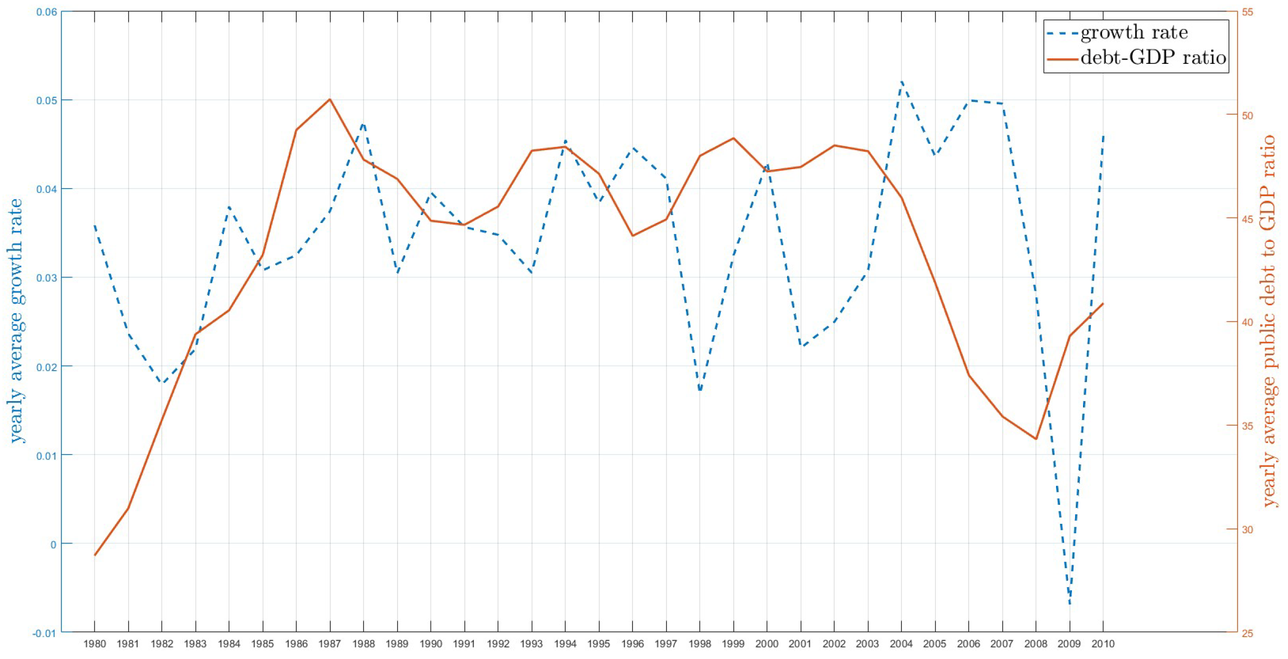
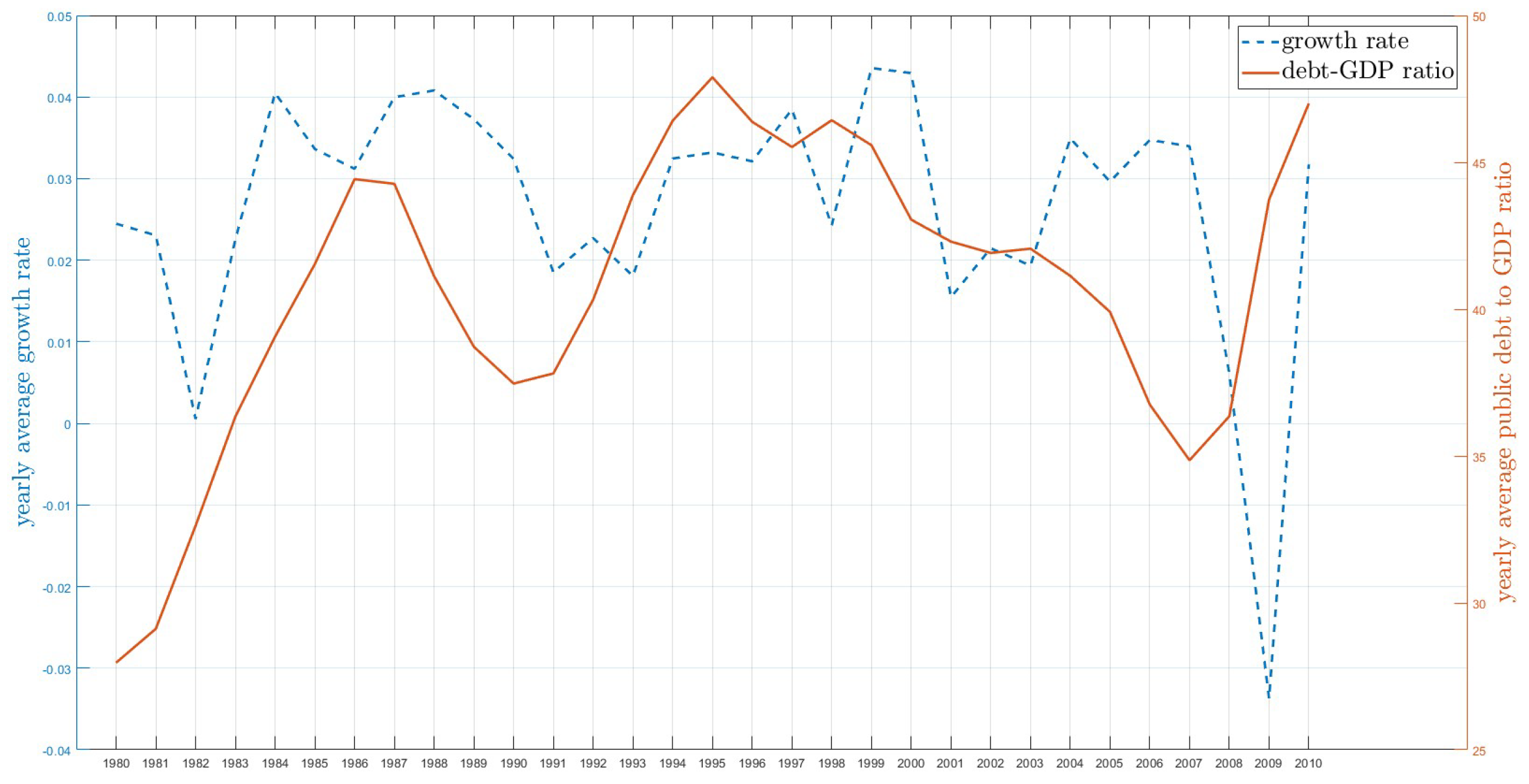
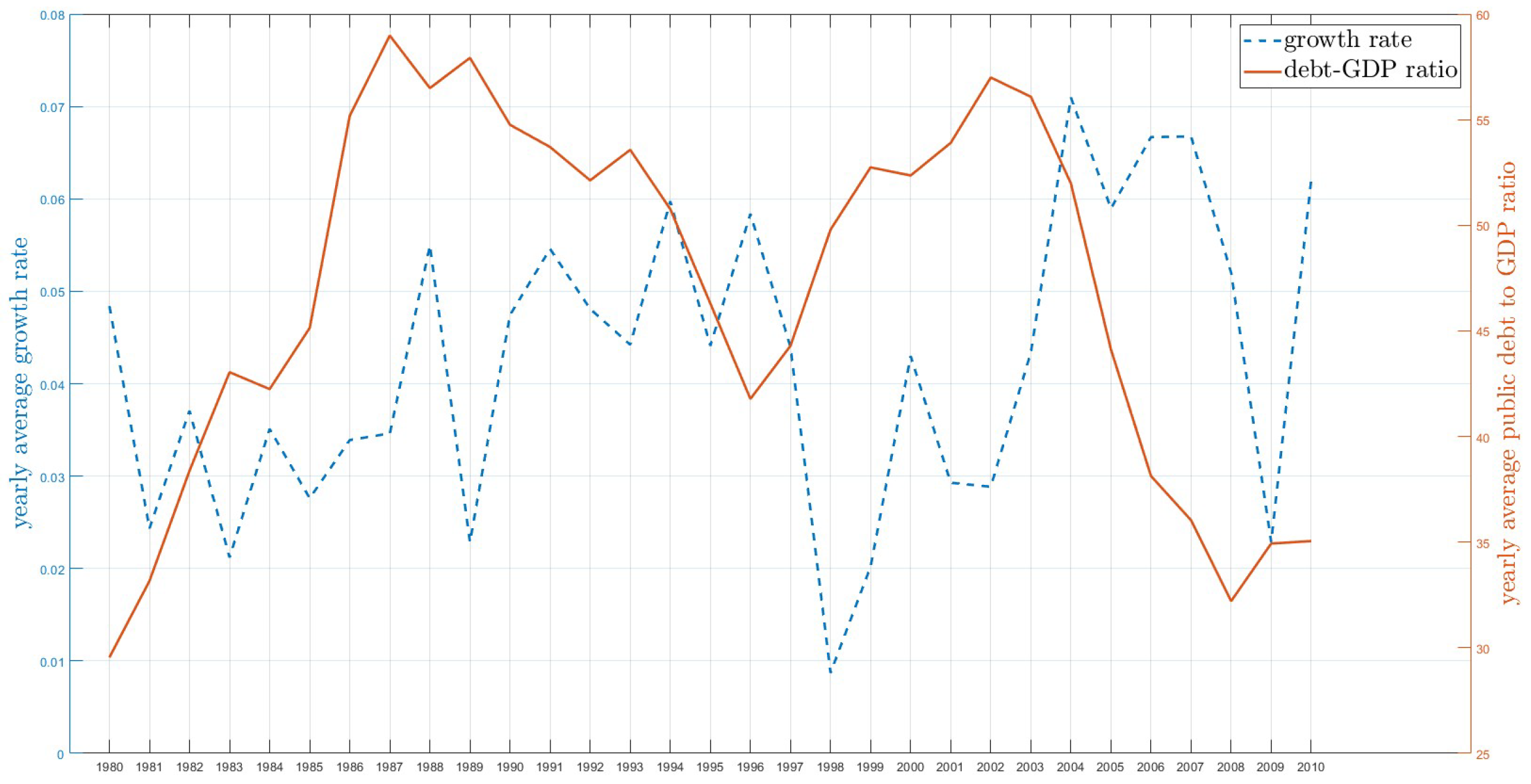
 Figure 1, Figure 2 and Figure 3 depict time-series plots of yearly average economic growth versus the yearly average public debt-to-GDP ratio for all countries, as well as separately for OECD and non-OECD countries. A visual examination of these plots reveals a common trend between the two variables, indicating that the public debt-to-GDP ratio captures the pattern of economic growth in all scenarios. However, a closer comparison of Figure 2 and Figure 3 reveals an asymmetric co-movement between these variables in OECD versus non-OECD countries, pointing to the club-based heterogeneity in the impact of public debt on economic growth. This observation motivates us to further explore the identification of unobserved group structures and the uncovering of group-based heterogeneity.

5.2. Identifying the Number of Groups

Since the true number of groups G 0 is unobserved, we follow Miao et al. (2020) and employ a BIC-type information criterion (IC) to ascertain the number of groups. This method is outlined as follows:
I C ( G ) = ln ( σ ^ 2 ( G ) ) + λ N T G K ,
where σ ^ 2 ( G ) represents the mean squared error for a given group number G and λ N T is the tuning parameter used for the penalty term.5 Then, the optimal number of groups is chosen by
G ^ = argmin G { 1 , , G max } I C ( G ) ,
where G max is the maximum number of groups, as determined by empirical research. Due to the data requirement, we set G max = 5 for the full sample, covering all countries, while for the subsamples, G max = 4 is applied separately to OECD and non-OECD countries. 
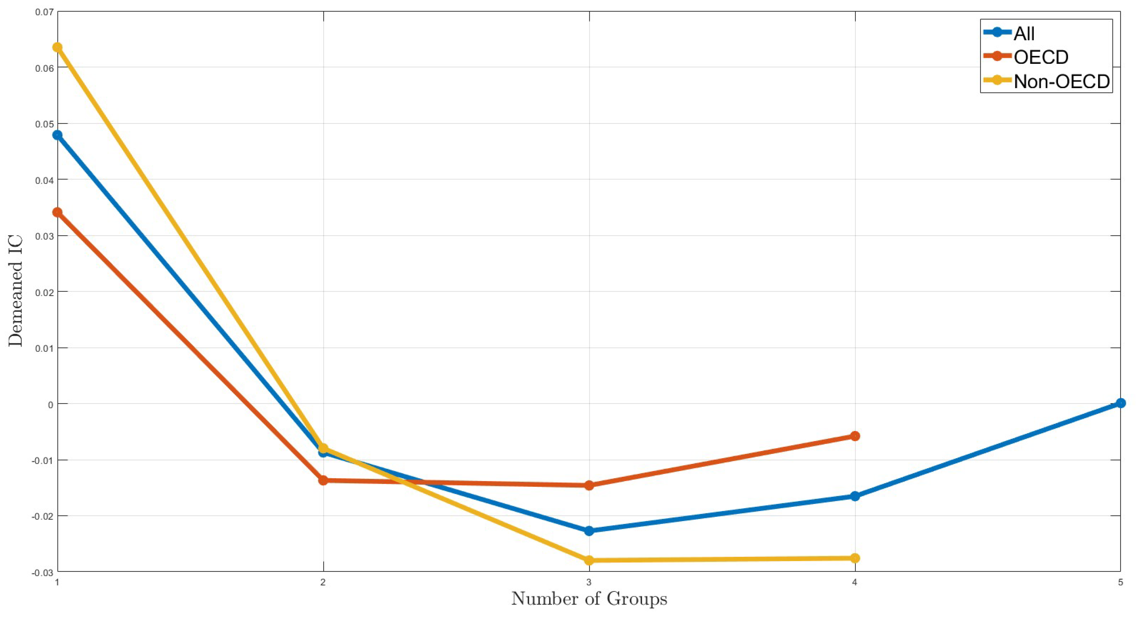
Figure 4 shows the de-meaned IC values for different numbers of groups, revealing that the IC curves reach their lowest point at G = 3 for all sample selections.6 Therefore, we select three as the optimal number of groups for our subsequent analysis.

5.3. Estimation Results

We then proceed to estimate the model (1) by setting G = 1 (indicating no latent group, our benchmark) and using G = 3 (as determined by the IC criterion). The results of these estimations using the full sample of all countries are summarized in Table 7.
Assuming a homogeneous kink threshold effect across all countries, we find the estimated tipping point to be 40.45%. However, in contrast to the conventional view, the pooled panel kink regression analysis reveals that higher public debt leads to lower growth in countries with lower debt levels and it appears to benefit economies with higher debt levels.
When analyzing the results of the panel kink regression with latent group structures, the estimations for group 1 align with the counter-intuitive results from the benchmark. The results suggest a negative impact on economic growth when a country’s debt-to-GDP ratio is below 43.51%, becoming insignificant above this level. However, only seven countries fall into group 1. The results for groups 2 and 3 are particularly notable, indicating threshold heterogeneity, where the impact of public debt on growth varies depending on the group members. Specifically, for group 2, the turning point is at 44.28%, where public debt fosters economic growth up to this level, after which the positive effect disappears. Group 3, with the highest threshold of 58.14%, exhibits a significant positive impact of public debt on growth when below this level, but this effect becomes insignificant once the threshold is exceeded. Notably, group 2 experiences a more substantial impact in the lower regime, indicating these countries benefit most from public debt. Consistent with the existing literature (e.g., Baum et al. 2013), our results for groups 2 and 3 indicate that while the impact of public debt on GDP growth is initially positive and statistically significant, it declines to near zero, and loses significance beyond specific public debt-to-GDP ratios.
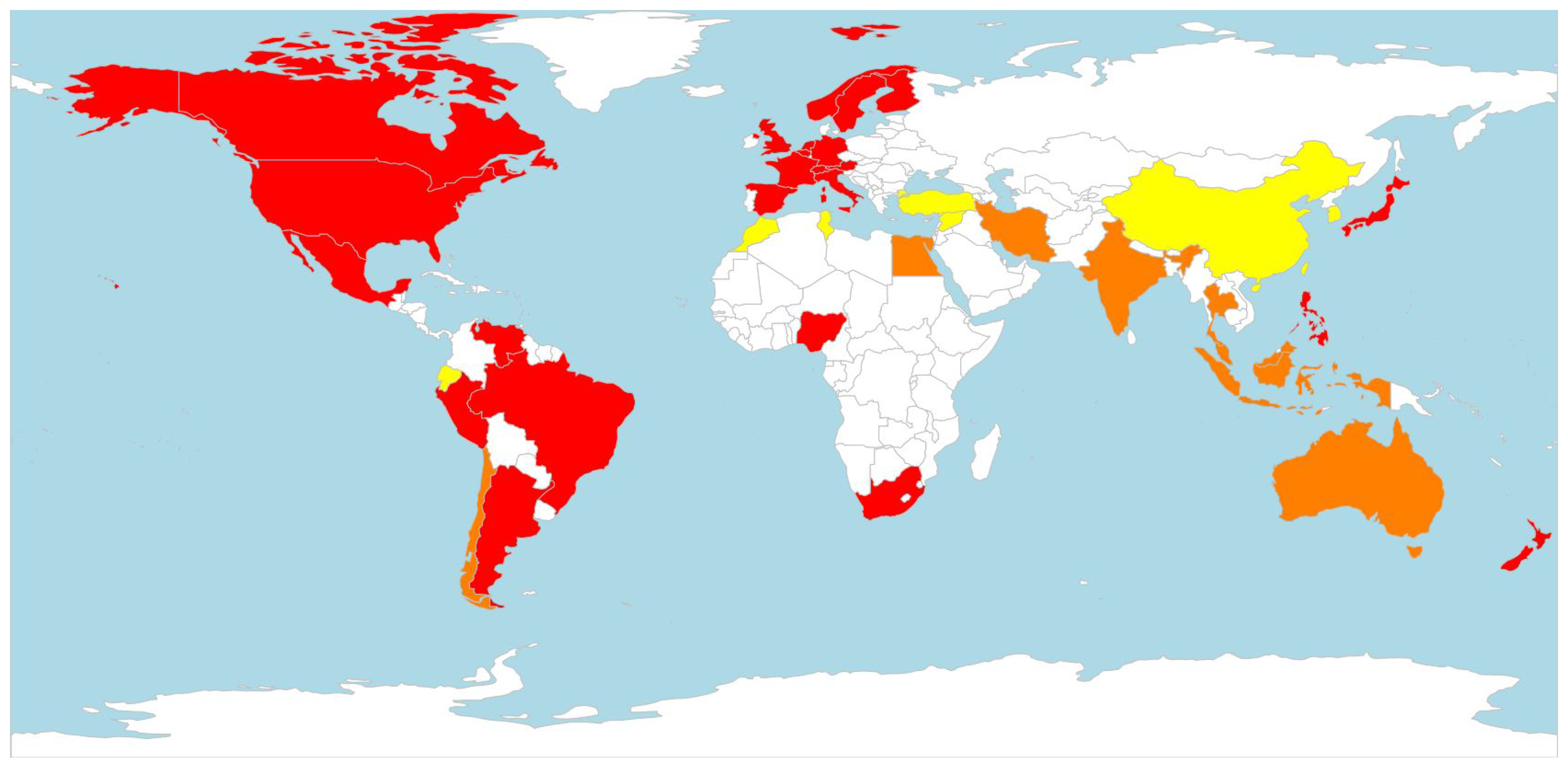
Figure 5 illustrates the world map with assigned group memberships. Interestingly, these classifications correlate to some extent with geographic location, economic development level, and the independence of the central bank. For instance, group 1, which includes countries like China and Turkey, is characterized by relatively weaker central bank independence. Group 2 is predominantly associated with the Indo-Pacific region. Meanwhile, group 3 encompasses the majority of the countries in the pan-American and European regions, indicating a distinct geographic and economic pattern in the grouping. In summary, the empirical findings emphasize the heterogeneity of threshold effects crucial in determining the influence of debt on growth.
As a robustness check on the impact of kink threshold heterogeneity, we also present the estimation results for OECD and non-OECD countries. The estimates from OECD and non-OECD countries are presented in Table 8 and Table 9, respectively. The estimation results reveal a distinct difference in the homogeneous kink threshold effect between OECD and non-OECD countries. Specifically, for OECD countries, the effect of debt on growth is insignificant in both regimes. In contrast, for non-OECD countries, the results are consistent with those of all countries shown in Table 7, showing a significantly negative impact in the low regime and a positive impact in the high regime, both at the 5 percent level. Turning to the results with latent group structures, none of the groups align with the findings that assume homogeneity for either OECD or non-OECD countries, indicating the presence of heterogeneity in threshold effects. Interestingly, within the low-debt regime, 16 of the 21 OECD countries (group 3, OECD) show a significantly positive impact of debt on growth at the 1 percent level. Conversely, public debt has a positive impact on growth in just 7 out of 19 non-OECD countries (group 3, non-OECD) at the same level, but the effect size is much larger. Furthermore, only 2 out of 21 OECD countries (group 2, OECD) exhibit a significantly negative impact of public debt on growth in the low-debt regime, compared to 4 out of 19 non-OECD countries (group 2, non-OECD). In the high-debt regime, an inverse U-shaped relationship is supported by the majority of OECD countries (group 3, OECD), where the positive impact of public debt on growth turns significantly negative at the 10 percent level once the debt-to-GDP ratio exceeds 54.58%. In non-OECD countries, the impact of debt on growth becomes insignificant in the high-debt regime for groups 1 and 2, while group 3 sees a significantly larger positive impact on growth when the debt ratio exceeds 61.4%. These results highlight the parallels between OECD and non-OECD countries and provide further evidence of the importance of accounting for heterogeneous kink thresholds. Ignoring these group patterns, as seen in the pooled panel kink regression results in all sample selections, could lead to counter-intuitive conclusions and erroneous policy implications.

6. Conclusions

This paper makes an important contribution to the ongoing debate regarding the nonlinear relationship between public debt and economic growth. While the existing literature primarily assumes a homogeneous threshold effect of public debt on economic growth, our approach diverges by employing a panel kink regression model that incorporates latent group structures. This method allows us to explore the heterogeneous threshold effects based on unknown group patterns. We propose a least squares estimator and demonstrate the consistency of estimating group structures. Our findings reveal that the nonlinear relationship between public debt and economic growth is characterized by a heterogeneous threshold level, which varies among different groups, highlighting that the mixed results found in previous studies may stem from the arguably incorrect assumption of a homogeneous threshold effect.
In future investigations, researchers might explore various potential extensions. Our proposed method concentrates solely on exogenous variables, potentially encountering limitations in an endogenous framework. In cases where threshold variables or regressors exhibit endogeneity, researchers may address this issue by employing the control function approach introduced by Zhang et al. (2023). Incorporating two or more endogenous threshold variables, as in Chen et al. (2023), can also be intriguing. Another avenue for exploration involves a dynamic latent group structure setup, allowing for changes in group composition over time. Lastly, one could delve into a KTR model featuring multiple kinks, with a notable challenge being the efficient identification of multiple thresholds while avoiding the computational burden associated with a grid search method.

Author Contributions

Conceptualization, C.C., T.S. and J.Z.; methodology, C.C., T.S. and J.Z.; Formal analysis, C.C., T.S. and J.Z.; investigation, C.C., T.S. and J.Z.; writing—original draft preparation, C.C., T.S. and J.Z.; writing—review and editing, C.C., T.S. and J.Z. All authors have read and agreed to the published version of the manuscript.

Funding

Thanasis Stengos acknowledges the financial support from NSERC of Canada [grant number: 401715].

Data Availability Statement

All data were obtained from Chudik et al. (2017) and were retrieved from https://doi.org/10.7910/DVN/UGHQLX (accessed on 5 November 2023).

Conflicts of Interest

The authors declare no conflict of interest.

Appendix A. Lemmas

In this section, we propose some lemmas which help to prove the theorems. Throughout the Appendix, let . denote the Euclidean norm. We use ( N , T ) to denote the joint convergence of N and N when N and N pass to infinity simultaneously. p , d , and ⟹ denote convergence in probability, convergence in distribution, and weak convergence, respectively.
First, we denote an auxiliary equation:
Q ˜ N T ( Θ , D , G ) = 1 N T i = 1 N t = 1 T χ i t ( γ g i 0 0 ) θ g i 0 0 χ i t ( γ g i ) θ g i 2 + 1 N T i = 1 N t = 1 T u i t
Lemma A1.
Under Assumptions 1 and 2, we have
sup ( Θ , D , G ) B G × D G × G N | Q N T ( Θ , D , G ) Q ˜ N T ( Θ , D , G ) | = o p ( 1 ) .
Proof. 
Note that
Q N T ( Θ , D , G ) = 1 N T i = 1 N t = 1 T χ i t ( γ g i 0 0 ) θ g i 0 0 + u i t χ i t ( γ g i ) θ g i 2 = Q ˜ N T ( Θ , D , G ) + 1 N T i = 1 N t = 1 T χ i t ( γ g i 0 0 ) θ g i 0 0 χ i t ( γ g i ) θ g i u i t .
Under Assumptions 1 and 2 and closely following the proof of lemma A.1 of Miao et al. (2020), we can show sup ( Θ , D , G ) B G × D G × G N 1 N T i = 1 N t = 1 T χ i t ( γ g i 0 0 ) θ g i 0 0 χ i t ( γ g i ) θ g i u i t = o p ( 1 ) , which concludes the proof. □
Lemma A2.
Suppose Assumptions 1 and 2 hold, we have d H Θ ^ , D ^ , Θ 0 , D 0 p 0 , where
d H Θ ^ , D ^ , Θ 0 , D 0 = max max g G min g ˜ G θ ^ g θ g ˜ 0 2 + | γ ^ g γ g ˜ 0 | 2 , max g ˜ G min g G θ ^ g θ g ˜ 0 2 + | γ ^ g γ g ˜ 0 | 2 .
Proof. 
Our proof essentially extends lemma A.2 of Miao et al. (2020) to allow for the continuous threshold effect. It suffices to show (i) max g G min g ˜ G θ ^ g θ g ˜ 0 2 + | γ ^ g γ g ˜ 0 | 2 = o p ( 1 ) and (ii) m a x g ˜ G m i n g G θ ^ g θ g ˜ 0 2 + | γ ^ g γ g ˜ 0 | 2 = o p ( 1 ) .
First, to show (i), based on the least squares estimator’s definition and the fact that ( Θ 0 , D 0 , G 0 ) minimizes Q ˜ N T ( Θ , D , G ) , we can show 1 N T Q ˜ ( Θ ^ , D ^ , G ^ ) Q ( Θ 0 , D 0 , G 0 ) = o p ( 1 ) .
Next, for any i = 1 , , N and γ D , as T , we can show
1 T t = 1 T β 1 , g i 0 0 d i , t 1 ( γ g i ) d i , t 1 ( γ g i 0 0 ) 2 = c 1 f ( γ g i 0 0 ) 2 | γ g i γ g i 0 0 | 2 + o p ( 1 ) , 1 T t = 1 T β 2 , g i 0 0 d i , t 1 + ( γ g i ) d i , t 1 + ( γ g i 0 0 ) = c 2 f ( γ g i 0 0 ) 2 | γ g i γ g i 0 0 | 2 + o p ( 1 ) ,
where c 1 and c 2 are some bounded constants.
By applying Assumption 2 (iv) and using Equation (A2), uniformly in ( Θ , D , G ) we have
Q ˜ N T ( Θ , D , G ) Q ˜ N T ( Θ 0 , D 0 , G 0 ) = 1 N T i = 1 N t = 1 T χ i t ( γ g i 0 0 ) θ g i 0 0 χ i t ( γ g i ) θ g i 2 = 1 N T i = 1 N t = 1 T θ g i θ g i 0 0 χ i t ( γ g i ) + β 1 , g i 0 0 d i , t 1 ( γ g i ) d i , t 1 ( γ g i 0 0 ) + β 2 , g i 0 0 d i , t 1 + ( γ g i ) d i , t 1 + ( γ g i 0 0 ) 2 c g = 1 G g ˜ = 1 G θ g ˜ θ g 0 M N T ( g , g ˜ , G , D ) θ g ˜ θ g 0 + c | γ g ˜ γ g 0 | 2 ,
where c = max { c 1 f ( γ g 0 ) 2 , c 2 f ( γ g 0 ) 2 } .
Thus, we have
o p ( 1 ) = c g = 1 G g ˜ = 1 G θ g ˜ θ g 0 M N T ( g , g ˜ , G , D ) θ g ˜ θ g 0 + c | γ g ˜ γ g 0 | 2 + o p ( 1 ) c g = 1 G g ˜ = 1 G max λ min M N T ( g , g ˜ , G , D ) , c θ g ˜ θ g 0 2 + | γ g ˜ γ g 0 | 2 + o p ( 1 ) c max g G g ˜ = 1 G max λ min M N T ( g , g ˜ , G , D ) , c θ g ˜ θ g 0 2 + | γ g ˜ γ g 0 | 2 + o p ( 1 ) c max g G min g ˜ G θ g ˜ θ g 0 2 + | γ g ˜ γ g 0 | 2 g ˜ = 1 G max c ̲ λ , c + o p ( 1 ) ,
where the last inequality is by Assumption 2 (v). This concludes the proof of (i).
To show (ii), redefine σ g = σ Θ ^ ( g ) argmin g ˜ G θ g 0 θ ^ g ˜ 2 + | γ g 0 γ ^ g ˜ | 2 in the proof of lemma A.2 of Miao et al. (2020). Following the same lines of arguments as in the proof of lemma A.2 of Miao et al. (2020), we can show, for all g ˜ G
min g G θ g 0 θ ^ g ˜ 2 + | γ g 0 γ ^ g ˜ | 2 θ σ 1 ( g ˜ ) 0 θ ^ g ˜ 2 + | γ σ 1 ( g ˜ ) 0 γ ^ g ˜ | 2 = min h G θ σ 1 ( g ˜ ) 0 θ ^ h 2 + | γ σ 1 ( g ˜ ) 0 γ ^ h | 2 = o p ( 1 ) ,
which implies (ii) and concludes the proof of this Lemma. □
Lemma A3.
Let g ^ i ( Θ , D ) = argmin g G t = 1 T y i t θ g χ i t ( γ g ) 2 . Suppose that Assumptions 1 and 2 hold. Then, for some η > 0 , we have
P r sup ( Θ , D ) N η 1 N i = 1 T I g ^ i ( Θ , D ) g i 0 = o ( T 4 ) ,
where N η = ( Θ , D ) B G × D G : θ g θ g 0 2 + | γ g γ g 0 | 2 < η , g G .
Proof. 
Our proof follows lemma A.3 of Miao et al. (2020). The only difference is the details of bounding Z i g ( Θ , D ) , where in our case
Z i g ( Θ , D ) = I ( g i 0 g ) I t = 1 T y i t χ i t ( γ g ) θ g 2 t = 1 T y i t χ i t ( γ g i 0 0 ) θ g i 0 0 .
Note that by simple calculation we can show
I t = 1 T y i t χ i t ( γ g ) θ g 2 t = 1 T y i t χ i t ( γ g i 0 0 ) θ g i 0 0 = I t = 1 T χ i t ( γ g i 0 ) θ g i 0 χ i t ( γ g ) θ g χ i t ( γ g i 0 0 ) θ g i 0 0 + u i t 1 2 χ i t ( γ g ) θ g θ g 1 2 χ i t ( γ g i 0 ) θ g i 0 0 = I t = 1 T χ i t ( γ g i 0 ) θ g i 0 χ i t ( γ g ) θ g 1 2 χ i t ( γ g i 0 ) θ g i 0 χ i t ( γ g ) θ g + χ i t ( γ g i 0 0 ) θ g i 0 0 χ i t ( γ g i 0 ) θ g i 0 + u i t 0 .
Therefore, for Z i g ( Θ , D ) , we have
Z i g ( Θ , D ) max g ˜ G { g } I L i ( g , g ˜ ) 0 ,
where
L i ( g , g ˜ ) = t = 1 T χ i t ( γ g ˜ ) θ g ˜ χ i t ( γ g ) θ g 1 2 χ i t ( γ g ˜ ) θ g ˜ χ i t ( γ g ) θ g + χ i t ( γ g ˜ 0 ) θ g ˜ 0 χ i t ( γ g ˜ ) θ g ˜ + u i t .
Then, closely following the steps taken by lemma A.3 of Miao et al. (2020) by using our defined L i ( g , g ˜ ) , for some constants C, we can show
Z i g ( Θ , D ) max g ˜ G { g } I t = 1 T χ i t ( γ g ˜ 0 ) θ g ˜ 0 χ i t ( γ g 0 ) θ g 0 1 2 χ i t ( γ g ˜ 0 ) θ g ˜ 0 χ i t ( γ g 0 ) θ g 0 + u i t H i T Z ˜ i g ,
where H i T = C η t = 1 T y i t 1 2 + d i , t 1 2 + x i t 2 + u i t 2 .
Then, by Assumption 2 (iv) and applying Equation (A2), we have
Pr ( Z ˜ i g = 1 ) g ˜ G { g } Pr ξ i T ( g , g ˜ ) H i T + o ( T 4 ) ,
where
ξ i T ( g , g ˜ ) = c 2 t = 1 T θ g ˜ 0 θ g 0 χ i t ( γ g 0 ) 2 + | γ g ˜ 0 γ g 0 | 2 + t = 1 T χ i t ( γ g ˜ 0 ) θ g ˜ 0 χ i t ( γ g 0 ) θ g 0 u i t .
Next, we show that the dominant term on the right-hand side of the preceding inequality is o ( T 4 ) . Let C 4 = 2 max i , t E ( y i t 1 2 + d i , t 1 2 + x i t 2 + u i t 2 ) , applying Assumption 2 (vii), we have
Pr ( Z ˜ i g = 1 ) g ˜ G { g } Pr ξ i T ( g , g ˜ ) H i T g ˜ G { g } Pr ξ i T ( g , g ˜ ) C C 4 η T + g ˜ G { g } Pr 1 T t = 1 T y i t 1 2 + d i , t 1 2 + x i t 2 + u i t 2 C 4 g ˜ G { g } [ Pr 1 T t = 1 T y i t 1 2 + d i , t 1 2 + x i t 2 + u i t 2 C 4 + Pr c 2 T t = 1 T θ g ˜ 0 θ g 0 χ i t ( γ g 0 ) 2 + | γ g ˜ 0 γ g 0 | 2 c 2 C ̲ g g ˜ + Pr 1 T t = 1 T θ g ˜ 0 θ g 0 χ i t ( γ g ˜ 0 ) u i t c 4 C ̲ g g ˜ + C C 4 η 2 + Pr 1 T t = 1 T β 1 , g 0 d i , t 1 ( γ g ˜ 0 ) d i , t 1 ( γ g 0 ) u i t c 8 C ̲ g g ˜ + C C 4 η 4 + Pr 1 T t = 1 T β 2 , g 0 d i , t 1 + ( γ g ˜ 0 ) d i , t 1 + ( γ g 0 ) u i t c 8 C ̲ g g ˜ + C C 4 η 4 ]
By Assumptions 1 and 2 and applying lemma C.1 of Miao et al. (2020), we can show the first two terms of the last inequality to be o ( T 4 ) . Let η [ min g G min g ˜ G { g } C ̲ g g ˜ 4 C C 4 ] and apply lemma C.1 of Miao et al. (2020), we can show the other three terms are of order o ( T 4 ) . The result then follows from the Markov inequality as used in the proof of lemma A.3 of Miao et al. (2020). □

Appendix B. Theorem

Proof of Theorem 1.
By Lemma A2, we have ( Θ ^ , D ^ ) N η . Therefore, we can apply Lemma A3 and have 1 N i = 1 N Pr ( g ^ g i 0 ) = o ( T 4 ) . This follows
Pr sup i I ( g ^ g i 0 ) = 1 i = 1 N Pr ( g ^ g i 0 ) = o ( N T 4 ) ,
which concludes the proof of this theorem. □

Appendix C. List of Countries

This table presents all the countries used in this paper.
Table A1. Countries used.
CountryOECDCountryOECD
Argentina Mexico
AustraliaMorocco
AustriaNetherlands
BelgiumNew Zealand
Brazil Nigeria
CanadaNorway
ChilePeru
China Philippines
Ecuador Singapore
Egypt, Arab Rep. South Africa
FinlandSpain
FranceSweden
GermanySwitzerland
India Syria
Indonesia Thailand
Iran, Islamic Rep. Tunisia
ItalyTurkey
JapanUnited Kingdom
Korea, Rep.United States
Malaysia Venezuela

Notes

1
Zhang et al. (2023) study the endogenous kink regression model by applying a nonparametric control function approach. Their method can be extended to our latent structure model. We leave this for future study.
2
Including x i t can be attractive for other applications. However, in our empirical study, we only include the constant term, assuming x i t = 0
3
We exclude the panel nonstationary regressors. Chen and Stengos (2022) study a threshold model with hybrid stochastic local unit root regressors. Their study offers a potential extension to the panel kink regression model. We leave this for future study.
4
Given the asymptotic equivalence holds, the asymptotic normality of the slope and kink threshold estimators can be derived by following Hansen (2017). We will not go through the details here.
5
In the empirical application, as suggested by Miao et al. (2020), we use λ N T = ln ( N T ) N T .
6
The IC values for various groupings are as follows: For the full sample of all countries, the IC values are −6.6269, −6.6835, −6.6975, −6.6913, −6.6747 for G = 1 , , 5 , respectively. For OECD countries, the IC values are −7.1278, −7.1756, −7.1765, and −7.1677, corresponding to G = 1 , , 4 . For non-OECD countries, the values are −6.3126, −6.3841, −6.4041, and −6.4037 for G = 1 , , 4 , respectively.

References

  1. Afonso, António, and João Tovar Jalles. 2013. Growth and productivity: The role of government debt. International Review of Economics & Finance 25: 384–407. [Google Scholar]
  2. Barro, Robert J. 1974. Are government bonds net wealth? Journal of Political Economy 82: 1095–117. [Google Scholar] [CrossRef]
  3. Baum, Anja, Cristina Checherita-Westphal, and Philipp Rother. 2013. Debt and growth: New evidence for the euro area. Journal of International Money and Finance 32: 809–21. [Google Scholar] [CrossRef]
  4. Blanchard, Olivier J. 1985. Debt, deficits, and finite horizons. Journal of Political Economy 93: 223–47. [Google Scholar] [CrossRef]
  5. Bonhomme, Stéphane, Thibaut Lamadon, and Elena Manresa. 2022. Discretizing unobserved heterogeneity. Econometrica 90: 625–43. [Google Scholar] [CrossRef]
  6. Bonhomme, Stéphane, and Elena Manresa. 2015. Grouped patterns of heterogeneity in panel data. Econometrica 83: 1147–84. [Google Scholar] [CrossRef]
  7. Caner, Mehmet, Thomas Grennes, and Fritzi Koehler-Geib. 2010. Finding the tipping point: When sovereign debt turns bad. Sovereign Debt and the Financial Crisis 63–75. Available online: https://papers.ssrn.com/sol3/papers.cfm?abstract_id=1612407 (accessed on 15 October 2023).
  8. Cecchetti, Stephen G., Madhusudan S. Mohanty, and Zampolli Fabrizio. 2011. The Real Effects of Debt. Bank for International Settlements Working Papers No 352. Basel: Bank for International Settlements. [Google Scholar]
  9. Chan, Kung-Sik. 1993. Consistency and limiting distribution of the least squares estimator of a threshold autoregressive model. The Annals of Statistics 21: 520–33. [Google Scholar] [CrossRef]
  10. Chan, Kung-Sig, and Ruey S. Tsay. 1998. Limiting properties of the least squares estimator of a continuous threshold autoregressive model. Biometrika 85: 413–26. [Google Scholar] [CrossRef]
  11. Chen, Chaoyi, and Thanasis Stengos. 2022. Estimation and inference for the threshold model with hybrid stochastic local unit root regressors. Journal of Risk and Financial Management 15: 242. [Google Scholar] [CrossRef]
  12. Chen, Chaoyi, Thanasis Stengos, and Yiguo Sun. 2023. Endogeneity in semiparametric threshold regression models with two threshold variables. Econometric Reviews 42: 758–79. [Google Scholar] [CrossRef]
  13. Chudik, Alexander, Kamiar Mohaddes, M. Hashem Pesaran, and Mehdi Raissi. 2017. Is there a debt-threshold effect on output growth? Review of Economics and Statistics 99: 135–50. [Google Scholar] [CrossRef]
  14. Eberhardt, Markus, and Andrea F. Presbitero. 2015. Public debt and growth: Heterogeneity and non-linearity. Journal of International Economics 97: 45–58. [Google Scholar] [CrossRef]
  15. Elmendorf, Douglas W., and N. Gregory Mankiw. 1999. Chapter 25 government debt. Handbook of Macroeconomics 1: 1615–69. [Google Scholar]
  16. Frankel, Jeffrey A., and David Romer. 1999. Does trade cause growth? American Economic Review 89: 379–99. [Google Scholar] [CrossRef]
  17. Gómez-Puig, Marta, Simón Sosvilla-Rivero, and Inmaculada Martínez-Zarzoso. 2022. On the heterogeneous link between public debt and economic growth. Journal of International Financial Markets, Institutions and Money 77: 101528. [Google Scholar] [CrossRef]
  18. Hansen, Bruce E. 2000. Sample splitting and threshold estimation. Econometrica 68: 575–603. [Google Scholar] [CrossRef]
  19. Hansen, Bruce E. 2017. Regression kink with an unknown threshold. Journal of Business & Economic Statistics 35: 228–40. [Google Scholar]
  20. Hidalgo, Javier, Jungyoon Lee, and Myung Hwan Seo. 2019. Robust inference for threshold regression models. Journal of Econometrics 210: 291–309. [Google Scholar] [CrossRef]
  21. Kourtellos, Andros, Thanasis Stengos, and Chih Ming Tan. 2013. The effect of public debt on growth in multiple regimes. Journal of Macroeconomics 38: 35–43. [Google Scholar] [CrossRef]
  22. Miao, Ke, Liangjun Su, and Wendun Wang. 2020. Panel threshold regressions with latent group structures. Journal of Econometrics 214: 451–81. [Google Scholar] [CrossRef]
  23. Panizza, Ugo, and Andrea F. Presbitero. 2013. Public debt and economic growth in advanced economies: A survey. Swiss Journal of Economics and Statistics 149: 175–204. [Google Scholar] [CrossRef]
  24. Reinhart, Carmen M., and Kenneth S. Rogoff. 2010. Growth in a time of debt. American Economic Review 100: 573–78. [Google Scholar] [CrossRef]
  25. Su, Liangjun, and Qihui Chen. 2013. Testing homogeneity in panel data models with interactive fixed effects. Econometric Theory 29: 1079–135. [Google Scholar] [CrossRef]
  26. Su, Liangjun, Zhentao Shi, and Peter C. Phillips. 2016. Identifying latent structures in panel data. Econometrica 84: 2215–64. [Google Scholar] [CrossRef]
  27. Zhang, Jianhan, Chaoyi Chen, Yiguo Sun, and Thanasis Stengos. 2023. Endogenous kink threshold regression. SSRN Electronic Journal. Available online: https://ssrn.com/abstract=4742634 (accessed on 1 February 2024).
Figure 1. Yearly average economic growth and public debt-to-GDP ratio: all countries.
Econometrics 12 00007 g001
Figure 2. Yearly average economic growth and public debt-to-GDP ratio: OECD countries.
Econometrics 12 00007 g002
Figure 3. Yearly average economic growth and public debt-to-GDP ratio: non-OECD countries.
Econometrics 12 00007 g003
Figure 4. The de-meaned IC values for identifying the number of groups.
Econometrics 12 00007 g004
Figure 5. Estimates of group memberships. Yellow signifies group 1, orange denotes group 2, and red is associated with group 3.
Econometrics 12 00007 g005
Table 1. DGP1 Monte Carlo simulation results: ( γ 1 , γ 2 , γ 3 ) = ( 1 , 1 , 1 ) .
Group 1Group 2Group 3
β 1 δ 1 γ 1 β 2 δ 2 γ 2 β 3 δ 3 γ 3
MSE
N = 50T = 300.0140.0300.2090.0070.0170.1260.4580.0350.336
N = 100T = 300.0100.0070.1070.0050.0030.0650.0070.0100.118
N = 50T = 600.0430.1410.1730.0040.0030.0510.0070.1860.170
N = 100T = 600.0020.0020.0270.0020.0010.0300.0030.0030.033
BIAS
N = 50T = 30−0.0190.0490.030−0.0140.0300.010−0.0690.0540.064
N = 100T = 30−0.021−0.011−0.037−0.0060.002−0.003−0.0100.0150.019
N = 50T = 60−0.0300.0530.012−0.0120.001−0.049−0.0100.0690.018
N = 100T = 600.0010.0090.0240.0010.0050.009−0.0130.004−0.026
STD
N = 50T = 300.1180.1660.4570.0850.1270.3550.6730.1800.576
N = 100T = 300.1000.0810.3250.0670.0570.2540.0810.0980.343
N = 50T = 600.2050.3710.4160.0660.0530.2190.0820.4260.412
N = 100T = 600.0420.0420.1630.0400.0370.1730.0510.0500.179
Table 2. DGP1 Monte Carlo simulation results: ( γ 1 , γ 2 , γ 3 ) = ( 0.5 , 1 , 1.5 ) .
Group 1Group 2Group 3
β 1 δ 1 γ 1 β 2 δ 2 γ 2 β 3 δ 3 γ 3
MSE
N = 50T = 300.1390.7310.3910.0240.4010.2880.0110.0430.255
N = 100T = 300.0160.0030.0990.0030.0030.0350.0060.0330.144
N = 50T = 600.0280.0100.1350.0050.0040.0740.0360.0340.173
N = 100T = 600.0070.0010.0550.0010.0010.0200.0010.0100.072
BIAS
N = 50T = 30−0.1000.1120.008−0.0160.1220.065−0.0280.051−0.044
N = 100T = 30−0.0250.0170.021−0.0030.0060.018−0.0180.030−0.005
N = 50T = 60−0.0360.008−0.013−0.0180.005−0.046−0.0190.0310.008
N = 100T = 60−0.0100.0090.0200.0010.0040.002−0.0040.025−0.005
STD
N = 50T = 300.1640.0980.3680.0690.0620.2680.1880.1820.416
N = 100T = 300.0850.0350.2330.0360.0360.1400.0330.0970.268
N = 50T = 600.3590.8470.6250.1530.6220.5330.1020.2000.504
N = 100T = 600.1240.0560.3140.0590.0520.1860.0760.1790.380
Table 3. DGP1 misclassification frequency (MF).
( γ 1 , γ 2 , γ 3 ) = ( 1 , 1 , 1 ) ( γ 1 , γ 2 , γ 3 ) = ( 0.5 , 1 , 1.5 )
N = 50N = 100N = 50N = 100
T = 300.00360.00210.01140.0088
T = 60000.0040.002
Note: The table reports the sample average misclassification frequency of our estimator across replications. For each replication, we define M F = 1 / N i = 1 N I ( g ^ i g i ) .
Table 4. DGP2 Monte Carlo simulation results: ( γ 1 , γ 2 , γ 3 ) = ( 1 , 1 , 1 ) .
Group 1Group 2Group 3
ρ 1 β 1 δ 1 γ 1 ρ 2 β 2 δ 2 γ 2 ρ 3 β 3 δ 3 γ 3
MSE0.0010.0090.0230.0040.0000.0110.0170.0030.0000.0160.0270.002
0.0010.0050.0110.0020.0000.0060.0130.0020.0000.0140.0150.002
0.0000.0020.0060.0020.0000.0030.0070.0010.0000.0040.0070.001
0.0000.0020.0040.0010.0000.0020.0040.0000.0000.0030.0050.001
BIAS0.0060.018−0.0680.0160.005−0.029−0.0370.036−0.001−0.0950.0070.040
0.0090.007−0.0600.0200.006−0.036−0.0620.0310.001−0.096−0.0150.041
0.001−0.011−0.0210.0150.002−0.022−0.0310.0160.001−0.047−0.0210.019
0.001−0.015−0.0260.0130.002−0.019−0.0360.0130.000−0.040−0.0340.017
STD0.0310.0940.1340.0580.0170.0990.1250.0380.0150.0810.1630.029
0.0210.0720.0850.0440.0120.0680.0940.0260.0100.0680.1230.024
0.0200.0480.0770.0390.0110.0470.0780.0240.0090.0470.0790.018
0.0130.0360.0540.0280.0080.0360.0480.0170.0070.0420.0640.015
Table 5. DGP2 Monte Carlo simulation results: ( γ 1 , γ 2 , γ 3 ) = ( 0.5 , 1 , 1.5 ) .
Group 1Group 2Group 3
ρ 1 β 1 δ 1 γ 1 ρ 2 β 2 δ 2 γ 2 ρ 3 β 3 δ 3 γ 3
MSE0.0010.0160.0110.0050.0000.0070.0180.0020.0010.0120.0530.006
0.0010.0060.0050.0030.0000.0060.0100.0020.0010.0070.0450.004
0.0000.0060.0040.0020.0000.0030.0070.0010.0000.0030.0260.002
0.0000.0020.0020.0010.0000.0020.0040.0010.0000.0020.0120.001
BIAS0.017−0.036−0.0460.0300.003−0.050−0.0530.032−0.022−0.080−0.0890.068
0.017−0.015−0.0450.0250.001−0.059−0.0420.035−0.020−0.067−0.1050.061
0.011−0.015−0.0210.0150.001−0.027−0.0370.015−0.011−0.041−0.0460.034
0.010−0.004−0.0250.0110.001−0.025−0.0360.015−0.010−0.035−0.0480.029
STD0.0280.1230.0950.0610.0160.0690.1250.0350.0150.0710.2130.036
0.0180.0750.0590.0440.0110.0460.0910.0250.0110.0500.1840.025
0.0170.0760.0620.0420.0110.0480.0780.0230.0090.0400.1540.020
0.0140.0460.0380.0280.0070.0350.0520.0160.0070.0330.0970.016
Table 6. DGP2 misclassification frequency (MF).
( γ 1 , γ 2 , γ 3 ) = ( 1 , 1 , 1 ) ( γ 1 , γ 2 , γ 3 ) = ( 0.5 , 1 , 1.5 )
N = 50N = 100N = 50N = 100
T = 300.00380.0050.0570.0539
T = 60000.0050.0064
Note: The table reports the sample average misclassification frequency of our estimator across replications. For each replication, we define M F = 1 / N i = 1 N I ( g ^ i g i ) .
Table 7. Estimated kink threshold and slope coefficients: all countries.
Latent Group
G1G2G3
γ 3.70203.77733.79064.0630
α 0.0190 ***0.0391 ***0.0402 ***0.0190 ***
(0.0023)(0.0055)(0.0053)(0.0026)
ρ 0.3366 ***−0.08420.3035 ***0.2975 ***
(0.0388)(0.0775)(0.0626)(0.0579)
β 1 −0.0057 **−0.0315 ***0.0147 ***0.0084 ***
(0.0028)(0.0044)(0.0044)(0.0029)
β 2 0.0076 **0.00220.00610.0032
(0.0037)(0.0083)(0.0077)(0.0066)
Country407924
Note: ***, and ** denote statistical significance at 1% and 5% levels, respectively. This table presents the results of the panel kink regression model estimations, both without and with latent group structures, using all countries. The optimal number of groups, determined to be 3, is based on minimizing the IC criterion by setting G m a x = 5 , as outlined in the results section. The first column shows the kink threshold and the slope parameters. The second column gives the results of the pooled panel kink regression model. The last three columns report the latent group estimates.
Table 8. Estimated kink threshold and slope coefficients: OECD countries.
Latent Group
G1G2G3
γ 3.63662.82894.49603.9997
α 0.0205 ***0.0304 ***0.0169 **0.0192 ***
(0.0026)(0.0068)(0.0070)(0.0022)
ρ 0.2864 ***0.04550.07680.2855 ***
(0.0539)(0.1289)(0.1047)(0.0600)
β 1 0.00050.0036−0.0239 ***0.0069 ***
(0.0030)(0.0074)(0.0075)(0.0026)
β 2 −0.00420.0217 ***0.0473−0.0102 *
(0.0042)(0.0082)(0.0389)(0.0059)
Country213216
Note: ***, **, and * denote statistical significance at 1%, 5%, and 10% levels, respectively. This table presents the results of the panel kink regression model estimations, both without and with latent group structures, using the subsample of OECD countries only. The optimal number of groups is 3 based on setting G m a x = 4 . The first column shows the kink threshold and the slope parameters. The second column gives the results of the pooled panel kink regression model. The last three columns report the latent group estimates.
Table 9. Estimated kink threshold and slope coefficients: non-OECD countries.
Latent Group
G1G2G3
γ 3.76853.82924.36914.1174
α 0.0224 ***0.0381 ***0.0314 ***0.0244 ***
(0.0038)(0.0062)(0.0070)(0.0058)
ρ 0.3078 ***0.3512 ***−0.17170.3224 ***
(0.0536)(0.0760)(0.1108)(0.0810)
β 1 −0.0111 **0.0166 *−0.0326 ***0.0256 ***
(0.0044)(0.0084)(0.0046)(0.0080)
β 2 0.0142 **−0.00490.02850.0530 ***
(0.0056)(0.0072)(0.0173)(0.0188)
Country19847
Note: ***, **, and * denote statistical significance at 1%, 5%, and 10% levels, respectively. This table presents the results of the panel kink regression model estimations, both without and with latent group structures, using the subsample of non-OECD countries only. The optimal number of groups is 3 based on setting G m a x = 4 . The first column shows the kink threshold and the slope parameters. The second column gives the results of the pooled panel kink regression model. The last three columns report the latent group estimates.
Disclaimer/Publisher’s Note: The statements, opinions and data contained in all publications are solely those of the individual author(s) and contributor(s) and not of MDPI and/or the editor(s). MDPI and/or the editor(s) disclaim responsibility for any injury to people or property resulting from any ideas, methods, instructions or products referred to in the content.

