1. Introduction
In economics, especially in the field of finance, time series modeling recurrently involves incorporating patterns of dependence in the conditional variance. In financial series, the so-called conditional volatility models are of particular interest, as variance plays a considerable role in determining asset prices, measuring risk and in the construction of tools to hedge them. By understanding the underlying factors driving the volatility dynamics, policymakers can implement measures to mitigate systemic risks and enhance financial stability. This may involve implementing macroprudential policies aimed at reducing excessive volatility and preventing financial crises.
However, as it is a latent process, conditional volatility is not easily estimated using conventional tools, which would include, for example, maximum likelihood estimators. In response, the literature presents the development of different paths regarding the treatment given to the assumed volatility process.
Among the proposed methods, one notable class is the family of univariate ARCH models (Autoregressive Conditional Heteroskedasticity), originally proposed by
Engle (
1982) and generalized into the univariate GARCH class (Generalized Autoregressive Conditional Heteroskedasticity) by
Bollerslev (
1986).
Another significant class of models treats conditional volatility as a stochastic process, commonly referred to as stochastic volatility (SV) models. Introduced by
Taylor (
1986) using a nonlinear state-space representation with the log-variance following an AR(1) process, univariate SV models offer certain advantages over the univariate ARCH class. They do not necessitate the assumption of a deterministic structure for latent variance, and using autoregressive formulations for the conditional variance, they allow for a more straightforward multivariate extension using formulations based on vector autoregressive (VAR) models and common factor structures. However, SV models come with greater complexity in their estimation due to the presence of latent variables in the likelihood of the process.
In the frequentist perspective, significant development centers around the quasi-maximum likelihood method based on prediction error decomposition via the Kalman Filter, independently proposed by
Nelson (
1988) and
Harvey et al. (
1994). Alternatively, Bayesian estimation techniques are particularly interesting because latent processes can be treated as additional parameters to be estimated. Refer to
Kim and Shephard (
1998) for the original Bayesian inference of SV models and, more recently,
Kastner and Frühwirth-Schnatter (
2014), both of which rely on Markov Chain Monte Carlo (MCMC) algorithms.
From an applied standpoint, simulation-based methodologies like MCMC can pose computational challenges, especially as the volume of data involved in the estimation grows in terms of dimensionality and the number of observations. These algorithms are susceptible to chain convergence issues, as highlighted by
Rajaratnam and Sparks (
2015), in addition to facing computational inefficiency due to the iterative and non-parallelizable nature of the method, resulting in longer execution times. Consequently, stochastic volatility models may become less appealing or even computationally prohibitive when dealing with very long series or multivariate formulations.
Martino et al. (
2011) propose an alternative approach to Bayesian estimation of stochastic volatility models using integrated nested Laplace approximations (INLA), originally introduced by
Rue et al. (
2009). This approach allows for the estimation of parameters and latent variables through precise deterministic approximations to the posterior distributions, provided that the model can be approximated by a Gaussian Markov random field. Notably,
Chaim and Laurini (
2019) highlights that the INLA method, based on an analytical approach, eliminates the need for simulation procedures, rendering it immune to issues related to chain convergence.
As the formulation used can be represented as a Gaussian Markov Random Field, it allows a representation using a conditional Markov structure (
Rue and Held 2005). The Markov property allows for representing the model’s precision matrix with a sparse matrix, which allows for the use of sparse linear algebra with relevant computational gains. Another important point is that Laplace approximations are numerically parallelizable, which allows all the computational power to be exploited using multiple processors.
The literature using this methodology has primarily focused on the analysis of the univariate case, where a single asset is considered in the state space formulation. However, extending the estimation of multivariate stochastic volatility models via integrated nested Laplace approximations is a natural progression, considering that works like
Martino et al. (
2011) only examine the bivariate case. Nevertheless, the dimensionality of the problem poses critical implications for the use of INLA in these models. As noted by
Martino et al. (
2011), the informational gain (greater volume of data and additional dimension) may lead to a substantial increase in estimation time, potentially undermining the efficiency of this tool.
One possible solution is to search for a more parsimonious parameterization, which allows the number of parameters to be estimated not to grow too much as the number of series analyzed also increases. Factor models fulfill exactly this role, as
Asai et al. (
2006) observes.
This study aims to develop a practical framework for estimating multivariate stochastic volatility models using a shared factors structure. The proposed formulation is based on a structure of common factors, where the log-volatility of each series is given by the combination of latent factors through a structure of estimated factor loadings. This structure can be implemented directly using the INLA methodology, taking advantage of all the computational gains related to the use of integrated Laplace approximations for parameters and latent factors, and also through the representation of sparse matrices and parallelism in the evaluation of the model that is possible through the Gaussian Markov Random Field representation of the proposed model. Through in-sample and out-of-sample analyses, we show the computational, fitting and forecasting gains derived from the proposed specification, compared to univariate specifications and the alternative multifactor formulation proposed by
Kastner et al. (
2017).
Our empirical focus centers on analyzing daily returns from stock exchange indices across various global regions. The primary objective is to uncover volatility interdependencies within these specified datasets while evaluating potential accuracy improvements compared to conventional univariate models. Additionally, we seek to assess the computational efficiency of our approach in comparison to commonly used MCMC algorithms.
The main contribution of the method is an efficient computational implementation for factor models of stochastic volatility, bypassing the computational cost and possible convergence problems existing in Bayesian estimations using MCMC. In this way, the proposed method can be used as an efficient computational tool for estimating risk, measured by conditional variance, in multivariate problems, with applications in portfolio allocation, construction of tail risk measures and hedging procedures.
This work is organized into five sections, beginning with this introductory section.
Section 2 provides a comprehensive review and discussion of existing literature concerning the estimation of stochastic volatility models, and the use of INLA (Integrated Nested Laplace Approximations), with a particular emphasis on the multivariate aspect within the context of factor modeling. In
Section 3, we offer a detailed exposition of the methodology to be employed, accompanied by an introduction to the datasets that will underpin the evaluation of our proposed models. The results of our analysis are presented in
Section 4, with in- and out-of-sample analysis using real data, preceding the final
Section 5 where we succinctly summarize the key findings.
2. Literature Review
Our exploration begins with the early developments in the estimation of SV models, followed by an examination of the integration of Bayesian methodologies and the application of the integrated nested Laplace approximation (INLA) method. Concluding this section, we provide an overview of the literature pertaining to multivariate and factorial models.
2.1. Stochastic Volatility Models
In general, the literature on stochastic volatility, especially concerning its theoretical foundations and principles, is well-established. Recent advancements are primarily associated with estimation methods.
Taylor (
1986) introduced the concept of stochastic volatility in the univariate case, assuming log-normal returns and a latent process of (log-)volatility. The unobservable nature of this process initially led to a search for methodological developments to overcome the limitations of traditional techniques, such as maximum likelihood. In this context, Bayesian inference techniques, in conjunction with Markov Chain Monte Carlo (MCMC) methods, gained popularity, fostering dedicated literature aimed at proposing more efficient alternatives. One such alternative is integrated nested Laplace approximations (INLA), introduced by
Rue et al. (
2009) and applied to stochastic volatility by
Martino et al. (
2011). This framework appears to offer accuracy at least on par with MCMC, as evidenced by
Ehlers and Zevallos (
2015), while also providing advantages in terms of estimation efficiency.
Starting from a sequence
of returns, the SV model of
Taylor (
1986) model can be represented as follows:
Log-variance, , is assumed to be a stationary first-order autoregressive process, whose dynamics are configured by the parameters (long-term average), (related to autoregressive persistence) and (marginal precision of the log-variance of ).
An immediate challenge arises from the unobservable nature of log-volatility. Following
Taylor’s (
1986) formulation, it is suggested to estimate
,
, and
(
) using sample moments, but not
. The impossibility of employing a maximum likelihood estimator is noted since it would necessitate dealing with a multiple integral with a dimension equal to the sample size to marginalize the latent variance vector.
Harvey (
1989) proposed a frequentist approach to address the issue of estimating the latent variable in the model. This approach involves a quasi-maximum likelihood estimator (referred to as “quasi-maximum likelihood”) based on prediction error decomposition via the Kalman Filter. To achieve this, the square of the log-returns is linearized, involving an average decomposition along with a first-order autoregressive process, thereby imposing a linear representation of the state space for the model.
Alternatively,
Sandmann and Koopman (
1998) discussed a methodology that replaces quasi-likelihood with a simulated version, called Monte Carlo Maximum Likelihood (MCML), which also allows for the application of the Kalman Filter in the decomposition of the prediction error.
Andersen et al. (
1999), on the other hand, returned to the class of estimators that aim to explore the moments of the sample, using the Efficient Method of Moments (EMM), in which the derivative of the log-likelihood function (score vector) provides the moment conditions. In the authors’ study, the EMM estimator achieves the efficiency of maximum likelihood estimators in large samples.
2.2. Multivariate and Factor Models
Since the inception of stochastic volatility models first proposed by
Taylor (
1986), several extensions have emerged, introducing a wider array of specifications and facilitating the multivariate analysis of conditional volatility patterns. Building upon the work of
Harvey et al. (
1994), multivariate SV modeling has gained momentum and undergone further developments, incorporating appropriate functional forms to capture specific stylized facts and presenting a more efficient approach to estimation and parameterization.
Amid these developments, the concept of factor structures has been introduced into the realm of multivariate stochastic volatility models, with greater emphasis given by
Jacquier et al. (
1995). These factor structures addressed the computational complexity associated with the high dimensionality inherent to multivariate volatility modeling.
Harvey et al. (
1994) laid the groundwork for what they referred to as a multivariate generalization of stochastic variance models. Drawing from the multivariate representation of ARCH models and the associated restrictions proposed by
Bollerslev (
1990),
Harvey et al. (
1994) assumed a set of equations to describe the model:
where
is the observation of the
i-th series in the period
t and the vectors
and
of errors follow a multivariate normal distribution with zero mean and covariance matrices
and
, respectively. It is also assumed that
has each element of its main diagonal equal to 1 and its other entries denoted by
. For estimation, the authors adopt a frequentist strategy, using a quasi-maximum likelihood estimator by means of the Kalman filter.
From a Bayesian perspective, the work carried out by
Martino (
2007) and
Martino et al. (
2011) introduced an estimation scheme based on the INLA methodology for the multivariate case. As opposed to the univariate formulation, adopted in the vast majority of works in which INLA is used, the multivariate model is capable of capturing a greater variety of data characteristics, for example, the spillover volatility effect, in which knowledge about one asset could help make predictions about another.
Martino (
2007) proposed a bivariate extension, written as
where
are the observed log-returns on
t,
and
are bivariate noise terms and
are the latent volatilities. Furthermore,
A generalization to larger dimensions was presented by
Shapovalova (
2021), who noted that this methodology might lose some of its computational efficiency advantages when applied to higher-order multivariate specifications.
Beyond the basic model, a variety of functional forms and specifications are possible, each making different assumptions about the correlation between volatilities and imposing distinct restrictions and parameterizations.
Asai et al. (
2006) identified and categorized these variants into four groups: asymmetric models, time-varying correlation models, factor models, and alternative specification models.
The first category of Multivariate Stochastic Volatility (MSV) models incorporates the asymmetries observed in the behavior of asset returns. Specifically, it accounts for the tendency for negative and positive variations to have different impacts on the volatility of the series, a concept known as the leverage effect, first identified by
Black (
1976). This phenomenon, which deals with a negative correlation between volatility and past returns was introduced to the stochastic volatility context by
Harvey and Shephard (
1996) and explored within the context of multivariate modeling by
Danıelssonn (
1998).
A second group of MSV models aimed to capture conditional correlations subject to variations over time, relaxing the assumption of constant correlations assumed in
Harvey et al.’s (
1994) basic model. One of the ways to do this, as proposed by
Yu and Meyer (
2006), is to use a Fisher transform for the correlation parameter.
So far, the categories we have discussed have been primarily driven by the goal of enhancing modeling flexibility rather than advancing computational efficiency in model estimation. Factor models, on the other hand, are designed to provide more parsimonious formulations with regard to the number of parameters involved in the problem.
Asai et al. (
2006) classified this category of Multivariate Stochastic Volatility (MSV) models into two types: multiplicative and additive models.
The first additive factor model can be traced back to
Harvey et al. (
1994) and was later expanded upon by
Jacquier et al. (
1995). This model begins with a factor-based structure for the
covariance matrix and
k active factors. The problem is formulated as follows:
In these equations, , with denoting the k univariate processes, and represents a matrix of factor loadings. The error term follows a normal distribution with zero mean and an identity covariance matrix of order m, with parameters given by . The authors estimated this model using Bayesian techniques, breaking down the posterior distribution into conditional distributions and employing a Metropolis–Hastings Markov Chain Monte Carlo (MCMC) sampling algorithm.
When compared to the basic MSV model by
Harvey et al. (
1994), the additive factor model stands out due to the fact that the number of parameters to be estimated grows only linearly as more return series are introduced into the analysis, i.e., as the dimension increases. In fact,
Asai et al. (
2006) demonstrated that, for the one-factor case, there are a total of
parameters, where
m represents the number of series. This makes the estimation of multivariate stochastic volatility models using methods involving simulation and chain convergence less computationally expensive.
Another aspect of factor models that moved in the same direction is the class of multiplicative models, partly inspired by the work of
Quintana and West (
1987). According to
Asai et al. (
2006), this class of MSV model involves separating log-returns into two components: a noise vector and a common factor.
Asai et al. (
2006) also discusses alternative specifications. The authors enumerate four alternative formulations for MSV models which rely on exponential matrix transformation, Cholesky decomposition, Wishart autoregressive process, and the observed range. In the first two cases, the motivation is to guarantee the construction of positive matrices defined for the covariance
, through the attribution of matrix exponential properties and Cholesky decomposition.
Another important category of approximate Bayesian inference methods is rooted in Variational Bayes (VB) techniques
Tan and Nott (
2018). VB frames the task of estimating the posterior distribution as an optimization problem, approximating the posterior density with a simpler distribution characterized by unknown parameters. This simplification often takes the form of a multivariate Gaussian distribution with an unknown mean and covariance matrix. Such an approach offers substantial computational advantages over traditional Markov Chain Monte Carlo (MCMC) methods. Moreover, VB can be integrated with sequential methods, facilitating parameter and latent state updates as new data points are observed. The application of Variational Bayes in the estimation of factor Stochastic Volatility (SV) models has been proposed in
Gunawan et al. (
2021), showcasing notable improvements in computational efficiency along with favorable fitting and prediction performance compared to MCMC-based approaches.
2.3. Bayesian Estimation and Integrated Nested Laplace Approximations (INLA)
In parallel with frequentist developments, several Bayesian estimation techniques have been proposed, capitalizing on the flexibility of Bayesian inference methods when dealing with models that include latent variables treated as additional parameters. However, MCMC approaches can encounter typical challenges such as slow chain convergence, owing to the high correlation among components of the latent volatility variable.
In addition to convergence issues, MCMC can also suffer from computational inefficiencies when applied to very large samples.
Martino et al. (
2011) suggested an alternative approach for estimating stochastic volatility models using integrated nested Laplace approximations (INLA), a methodology originally introduced by
Rue et al. (
2009). As long as models can be approximated or represented as Gaussian Markov random fields (GMRF) (see
Rue and Held (
2005) for the definition and properties of GMRF) both parameters and latent factors can be estimated. The advantage of this approach lies in its utilization of analytical calculations (eliminating the need for simulations) with sparse matrices and operations that are easily parallelizable.
As demonstrated by
Rue et al. (
2009), through conditional representation, the precision matrix
is typically sparse, with only
of the
entries being non-zero in most cases. Furthermore, it can be factorized as
, where
represents the lower Cholesky triangle, inheriting the sparsity of the precision matrix.
Starting with the standard model of stochastic volatility, which includes the equations for
and
, the proposition of
Martino et al. (
2011) is extended by assigning a Gaussian prior distribution to the mean parameter
, with zero mean and known variance. Consequently, the standard model can be interpreted as a latent Gaussian model in which the latent field
x is defined as:
and
are parameters behind volatility. The latent Gaussian field determined by
is partially observed through the conditionally independent data set
, where
n denotes the number of observations, with likelihood
and
are process parameters
. Considering
, stochastic volatility models can be evaluated by calculating the marginal distributions
The INLA approach can then be used to perform inference on marginals of
, allowing accurate approximations for
,
and
, due to its Gaussian approximation for densities given by the form
where
. In the context of stochastic volatility models and the formulations discussed by
Martino et al. (
2011), the precision matrix
is tridiagonal, in addition to having the last row and the last column with non-zero values. Still, the vast majority of entries in this matrix continue to consist of zeros, so that
is sparse.
Given this structure, the model can be estimated using the INLA methodology proposed in
Rue et al. (
2009). For space reasons, we do not present the INLA methodology, but details can be obtained in
Rue et al. (
2009) and recent developments in the implementation of the method in
Van Niekerk et al. (
2023).
In general, there is a consensus regarding the speed advantages of INLA over MCMC, as explicitly measured in studies like
Rue et al. (
2009) and
Chaim and Laurini (
2019). In the former work, taking into account code compilation time, INLA was approximately eight times faster in each estimation compared to MCMC. In the latter study, which analyzed the computational cost of SV models, the computation gains were on the order of 25 times, marking a substantial difference. In terms of estimation accuracy,
Ehlers and Zevallos (
2015) found improvements associated with the INLA method, particularly when calculating a Value-at-Risk (VaR) metric, comparing it with a quasi-maximum likelihood estimator. Similarly,
Chaim and Laurini (
2019) investigated the method’s accuracy for series with long memory, this time in comparison to traditional MCMC techniques, and found comparable performance between the two.
Furthermore, there has been a growing body of literature focusing on the practical applications of the INLA methodology, with an emphasis on implementations in the R language, using the R-INLA package
1. Among these contributions,
Ruiz-Cárdenas et al. (
2012) introduced a general computational approach for Bayesian inference using R-INLA for time series models, expanding the range of dynamic models accessible through the tool.
Martins et al. (
2013) documented some of the functionalities and resources added to the package since its initial versions. Specifically, within the context of stochastic volatility models,
Ravishanker et al. (
2022) has provided practical estimation guides and code examples for execution in R, covering modeling with both Gaussian errors and heavy-tailed distributions, such as Student’s t distribution.
3. Proposed Model and Methodological Aspects
Seeking to achieve the objectives of establishing a feasible and efficient way of estimating multivariate stochastic volatility models, we adapt the methodology based on integrated nested Laplace approximations for the case of multifactor formulations. In principle, such models can be built using formulations close to the univariate case, increasing the number of observation (state) equations and incorporating latent factor structures.
3.1. Benchmark and Starting Point
The work starts from a specification similar to that presented by
Kastner et al. (
2017) and
Hosszejni and Kastner (
2021), which served as a benchmark model. The authors build a structure for efficient estimation via MCMC of a model with
m series and
k factors. They are defined as
is a vector with the mean parameters,
is a vector of latent factors and
is a
matrix of factor loadings. The following diagonal covariance matrices are also assumed:
For identification reasons concerning the time-varying covariance matrix
2 (
), we impose some restrictions on parameters, such as setting the level of log-variances to zero, that is,
(
. In addition,
Kastner et al. (
2017) frees the loading matrix
, in order to identify only sign changes between its elements. See
Frühwirth-Schnatter et al. (
2023) for further discussion of identification structures in factor models.
To proceed with the estimation,
Kastner et al. (
2017) defined the prior distributions for the mean parameters, unobserved variances and factor loadings. In the case of
, Gaussian distributions are chosen, with
, where
is a vector of means and
is a variance-covariance matrix. Regarding the latent variance parameters, notably the persistence of the series (
and
), a prior of type
, that is, the Beta distribution. The choice is justified by the objective of avoiding non-stationarity in the variance process, which implies limiting
to the interval
. According to
Hosszejni and Kastner (
2021), since financial series tend to present very persistent variances, with values of
close to 1, it is possible to establish an informative prior distribution by choosing
and
, such that higher values for
would be more likely.
The distributions for the log-variance volatility,
, and its initialization parameter,
, are also specified. The
gamma and normal distributions are used, respectively, in such a way that:
assuming
stationary, an assumption that can be relaxed by defining a prior of the type
, with
representing a constant variance. Finally, regarding the prior behind the loading matrix
, independent and zero-centered Gaussian distributions are adopted (
), and are an important point for identifying the factor variance, as reported by
Kastner et al. (
2017).
The estimation of parameters through MCMC sampling employs a Metropolis–Hastings scheme, bolstered by interweaving strategies from
ASIS3, aimed at mitigating issues related to slow chain convergence. Practical implementation can be carried out in the
R programming language using the factorstochvol package (See
Hosszejni and Kastner 2021). This package facilitates the easy configuration of hyperparameters, model identification structure, and sampler adjustments, as well as enabling predictions within and outside the observed sample. The sampler is coded in
C++, offering superior execution speed for the draw stage (
draws), which is typically computationally intensive.
From a theoretical standpoint,
Kastner et al. (
2017) presented an algorithm for conditional MCMC sampling in four steps, commencing with the selection of initial values for
,
,
,
,
, and
. In the first stage, the
m idiosyncratic variances
are estimated, still in the univariate context, alongside the parameters
,
, and
(
). Similarly, this process is repeated for the
r factor variances, along with their parameters
and
, with
. The second step entails sampling for each row
of the factor loadings matrix, beginning with
. It is important to note that this step involves estimating
m multivariate regressions, each with dimension
and based on
T observations, where
represents the number of unconstrained elements in
.
Following this initial sampling process, new samples are drawn for each element on the main diagonal of
using the interweaving approach, either in relation to the equation of state for the factors or concerning latent volatilities. The first case is referred to as shallow interweaving, while the second is termed deep interweaving, as defined in
Kastner and Frühwirth-Schnatter (
2014). Both strategies aim to accelerate the convergence of Markov chains by re-sampling the parameters conditioned on latent variables of the model in a reparametrized version of the model, with deep interweaving generally preferred in most cases. Finally, the last step of the algorithm involves drawing samples for
from
(
), entailing the estimation of an additional
T r-dimensional multivariate regressions, each with the number of observations equal to
m, representing the number of series in the analysis.
It is worth noting that in step 1,
univariate stochastic volatility models are used, which
Kastner et al. (
2017) combine with two other observation equations:
and
and
are, respectively, innovation terms associated with
and
. The iteration of the algorithm then results in samples from the joint posterior distribution, with the discarding of the burn-in samples in order to avoid any influences from initial values.
3.2. Proposed Formulation
In the context of this study, an alternative formulation has been chosen, where the factor loadings are directly estimated within the latent volatility equations. In general terms, the proposed model, featuring
m series and
k factors, is represented as follows:
where
represents a vector containing the
m log volatilities,
denotes a mean parameter, and
is a
matrix of factor loadings. Diagonal covariance matrices
and
are permitted, indicating independent stochastic volatility processes. As for the factor log volatilities, denoted by
, we have:
where
represents a diagonal matrix of persistence parameters, and thus a univariate first-order autoregressive structure for each factor. The relationship between the return equations, represented by the vector
, and the volatilities for each asset is expressed through the matrix
, which is of size
:
The selected functional forms maintain the desirable properties of the modeling approach using INLA. As argued by
Martino (
2007), there is a possibility of losing the computational advantage associated with the method in its original form, due to the curse of dimensionality. Therefore, more parsimonious models can help mitigate inefficiencies arising from the dimensionality increase, potentially yielding benefits from increased information compared to univariate modeling. Furthermore, these proposed models can be implemented using the R-INLA package and its existing functionalities.
For the estimation process, we begin with two fundamental identification restrictions: the number of factors must be less than or equal to the number of return series
, and for one of these series, the load parameters
are fixed on unitary values. Following the implementation procedure of the INLA methodology, the proposed model is reinterpreted as a Gaussian Markov random field model in three stages, as adopted by
Martino (
2007). In the first stage, a likelihood model is defined:
where
is a vector of hyperparameters related to volatility.
Next, the latent fields referring to
and
are modeled. Then we have:
with
and
as hyperparameter vectors associated with their respective covariance matrices (
and
), Gaussian prior distributions are assumed for the mean parameters (
), centered on zero. Consequently, as demonstrated by
Martino (
2007), the average volatility can be incorporated into the latent field by calculating the following density:
where
represents the precision matrix, and
denotes the latent field for volatility. The sparsity of
offers computational efficiency, a property explored in greater detail by
Rue and Held (
2005) and
Rue et al. (
2009).
In the final stage, a prior
is established for the hyperparameter vectors
. In this context, the study assumes distributions in line with the proposals by
Martino (
2007) wherever applicable, particularly regarding parameters related to the factor structure. However, for compatibility with the
R-INLA package, the precision parameter (
) is handled in terms of its natural logarithm (log-precision), representing a non-informative prior for the precision, and the persistence parameter (
) is transformed using a function defined between
and 1, as follows:
the prior distributions of the other parameters are Gaussian. Given the latent field
, the estimation via INLA involves building an approximation for
from
and from
.
To obtain the joint posterior distribution in relation to the hyperparameters, we start from the following Gaussian approximation for the complete conditional density of
:
is a normalization constant,
corresponds to the mode of
and
is a band matrix with width equal to the number of series
m, due to the Markov structure derived from the conditional density, which can be written as:
where
contains the
order terms in the Taylor expansion
around
in the Hessian. In this way, the joint posterior for
can be approximated through the following relationship:
The approximation for
, on the other hand, follows a Gaussian strategy but can take advantage of the results obtained in the evaluation stage
. In particular, we take
as the mean parameter for the distribution, leaving only the values for the marginal variances, represented by
. The calculation is performed according to the recursive methods proposed by
Rue and Martino (
2007), allowing the approximation to be given by:
It is worth pointing out, however, that, according to the authors, this approximation is not accurate in some situations, especially when there are extreme values for . Its merit lies in constituting a faster alternative to other more precise ways of performing the calculation, which is especially interesting in the context of models in which dimensionality is a relevant issue.
Finally,
can be approximated, once
and
, through a numerical integration of the type:
to be performed on a set of points (
grid) for
, with the weights
being equal to 1 for equidistant points. However, in order to speed up the approximation process, we adopt an approach based on the empirical Bayes procedure, in which only one integration point equivalent to the posterior mode of hyperparameters is used. In general terms, the term
is replaced by
, with
being the mode of
. According to
Martino (
2007), the approach is highly accurate when the distribution of the hyperparameter vector conditional on the log-returns is regular.
3.3. Practical Implementation
From the perspective of practical implementation, the R-INLA package allows more efficient strategies to be defined from a computational point of view with the help of the argument control.inla, which controls the way in which numerical approximations and integrations are computed. Among the options of interest for the work, the integration approach via the empirical Bayes procedure is achieved through the command control.inla = list(int.strategy = “eb”), while the Gaussian approximation for is chosen by the argument strategy = “gaussian”. The complete list of arguments considered in the estimation can be seen in the code used:
![Econometrics 12 00005 i001]()
In addition to the settings already mentioned regarding the strategies for obtaining approximations, one more argument is defined, referring to the reordering algorithm chosen for the precision matrix. The option is to use the METIS implementation
4, which aims to evaluate sparse matrices efficiently, both in terms of storage needs and processing capacity. The fact that METIS reordering is perfectly suited to parallelization stands out, reinforcing the efficiency aspect of matrix operations.
The model is estimated using a multiple likelihood structure, with the same configuration for vectors and indices, regardless of the number of factors taken into account in the analysis. Assuming a general case involving
m series,
k factors and
n observations for each return series we have, as a starting point, the creation of a return matrix of dimensions
, organized as follows:
refers to the log-return of asset
i, for the period
t, and null entries in the matrix are denoted by
NA. It should also be noted that the first
n lines of
correspond to null values, such that the first entry referring to a return,
, appears in line
of the matrix, since in this representation the first
n lines of
represent the unobserved values of the latent factors, treated as missing values and estimated by the Bayesian inference procedure. This formulation implies that the latent factors will be associated with all observed series via the factor loadings structure as copies weighted by the parameters representing the factor loadings of these unobserved variables.
Three other groups of indices are constructed, in parallel, with the purpose of estimating the fixed and random effects of the linear dynamic model. Regarding the fixed effects, we have the following
m vectors:
where the first
n elements are left as null values and, for each vector
, a sequence of 1’s with dimension
n and starting from element number
. Furthermore, other
k identical indices associated with the evolution of the factors are added and initialized as follows:
the first
n elements being the sequence from 1 to
n, in a structure that is repeated for all
, with
. Finally, the random effects with respect to log variances are captured by a set of
vectors, constructed as:
Even if it is true that for the same index
i of assets,
,
, it is possible to use the same definition of indices for any number
of factors as long as this last vector structure is created according to the case in which there are as many factors as series in the analysis (
), taking the number of vectors to
. An adjustment would be necessary, however, in the sense of manually assuming that the factors disregarded in the estimation are set to zero, that is, that they have a log-precision set at a high value and their persistence parameter is fixed and equal to zero. See
Ruiz-Cárdenas et al. (
2012) for details on this structure.
Once the necessary vectors have been constructed, the formula that will enable the estimation of the model is written based on the return matrix and the indices created. In the context of the R-INLA package, terms related to random effects are indicated by the function f(), which takes as arguments the respective index vector, a string of characters informing the model that describes it and additional specifications about parameters. Taking the general case where , the formula can be written as:
![Econometrics 12 00005 i002]()
In this formulation, the models behind the indices of each log-volatility vector are constructed as copies of the structure established for a vector of indices associated with the factors through the attribute copy, which allows for the inclusion of a shared component between more than one linear predictor. Furthermore, it is observed that the models for the vectors of the group have, for each factor j, one of its terms (the first, in this case) presenting fixed hyperparameters, respecting restrictions imposed on factor loadings. For the group of , it is necessary to define the argument “model = “ar1””, which determines a first-order autoregressive structure for the factor log variances.
4. Results
In this section, we analyze the empirical results of estimating the proposed multivariate model, considering specifications with one to four latent factors, using the representation given by the Equations (
25) and (
26). We compare these results with models estimated using Markov Chain Monte Carlo (MCMC) using the multifactor representation proposed by
Kastner et al. (
2017) and also with the results of a univariate-based specification. The comparison is based on both in-sample and out-of-sample fit measures, as well as model selection metrics using information criteria.
4.1. Data Description
The empirical part of the work makes use of daily data for stock exchange index quotes
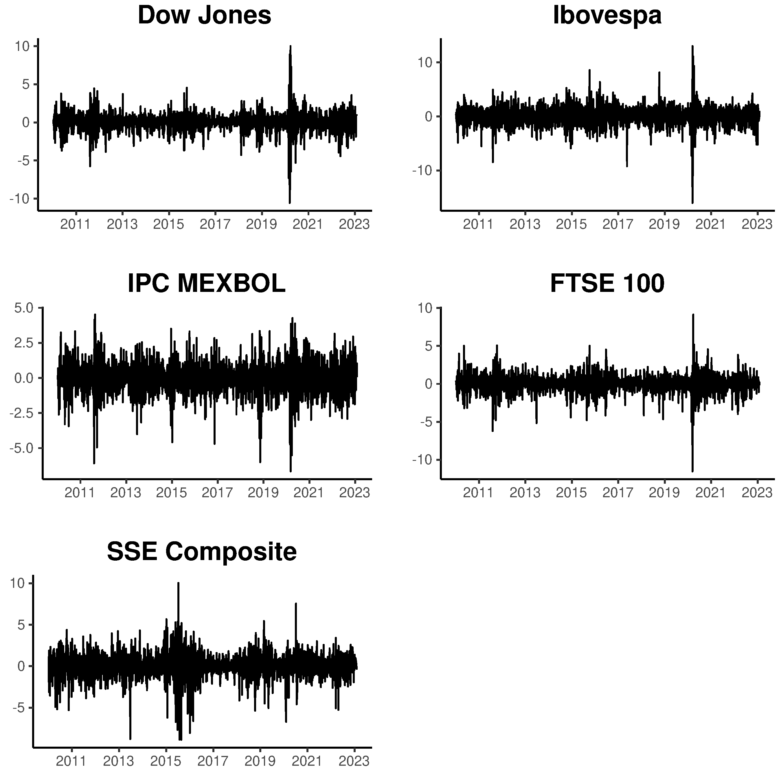
5, over the same time interval. The log-returns for indices representing different markets and from different parts of the globe were selected as variables, namely: Dow Jones Industrial (United States), Ibovespa (Brazil), Índice de Precios y Cotizaciones (Mexico), FTSE 100 (England) and SSE Composite Index (China). In
Table 1, these indices are listed, and abbreviations are given to them in order to facilitate their identification and denotation.
The analysis covers the daily closing returns of each index from January 2010 to February 2023, representing a sample of 2737 observations for each variable. This time span ensures a sufficient volume of data for the number of series analyzed, facilitating an adequate assessment of the proposed model in terms of computational efficiency.
Figure 1 displays the index returns between the specified dates.
The selected indices are widely used in the global financial market and represent various regions worldwide. Additionally, they consider the potential for interaction among them in terms of contagion and spillover effects on the price volatility of traded assets. For indices like Ibovespa and Dow Jones Industrial,
Achcar et al. (
2012) highlight the significance of their relationship in establishing investment references for emerging markets.
Table 2 provides descriptive statistics associated with the log returns of the selected indices, including mean, median, standard deviation, skewness, kurtosis, and the number of observations. A Jarque–Bera test is also conducted, with the computed values presented in the table. In all cases, the null hypothesis of Gaussian distribution is rejected at a significance level of
.
4.2. Empirical Analysis
To analyze the results obtained from the formulation of stochastic volatility models based on the proposed multifactor structure, we examine various specifications for the latent factor structure. We initiate with a structure featuring only one factor and gradually expand the latent factor structure until we reach a model with four factors, using the model represented by Equations (
25) and (
26) with varying numbers of latent factors. Additionally, we estimate a model based on univariate stochastic volatility (SV) models, which is based on assuming that each observed series only depends on a single latent factor that is unique to this series, but where we estimate these five univariate SV processes jointly using INLA. We compare the in and out of the sample performance of the multivariate factor structure proposed by
Kastner et al. (
2017) using MCMC methods.
Table 3,
Table 4,
Table 5 and
Table 6 provide a summary of the Bayesian posterior distribution of estimated parameters using INLA for the models with one to four latent factors, while
Table 7 presents the results for the specification based on univariate SV models. In each table, we present the mean, standard deviation, quantiles at 0.25, 0.5, and 0.975, and the mode of the posterior distribution for each model parameter. Furthermore, we include the marginal likelihood (MLIK), the Deviation Information Criterion (DIC), and the Widely Applicable Information Criterion (WAIC), also known as the Watanabe–Akaike information criterion, for each model. The DIC and WAIC are information criteria frequently used in the context of Bayesian estimation, being a generalization of the Akaike information criterion (AIC). See
Ando (
2007);
Spiegelhalter et al. (
2014) for the definition and properties of DIC and
Watanabe (
2010) for the WAIC.
We initiated a comprehensive analysis, focusing on the overall model fit, which was measured by marginal likelihood, and model fit was penalized by model complexity, as measured by DIC and WAIC criteria. As expected, the marginal likelihood indicates a better fit for the more complex models, with the model featuring four factors achieving the highest value, calculated as −19,966.49. Additionally, it is worth noting that the model with a single common factor obtains a marginal likelihood of −20,277.92, surpassing that of the model based on univariate stochastic volatility (SV) models, which is calculated as −20,513.56. This indicates that the common factor structure provides an advantage over univariate SV models when considering this model fit criterion.
The DIC and WAIC information criteria also favor more complex models, with the model featuring four latent factors emerging as the best model according to these two criteria. It has DIC and WAIC values of 38,738.78 and 38,766.12, respectively. Even when accounting for greater complexity in the model, models with more latent factors demonstrate a superior fit.
To perform an in-sample disaggregated comparison for each analyzed series and to verify the results of the adjustment of the multifactor models estimated by Markov Chain Monte Carlo (MCMC) using the structure proposed in
Kastner et al. (
2017), we present
Table 8. The table includes the mean error (ME), root mean squared error (RMSE), and mean absolute deviation (MAE) between the absolute value of each return series (taken as a proxy for the true unobserved volatility) and the volatility estimated by the models in our analysis. Bold values denote the best results for each measure in all analyses. We consider the multifactor models with one to four latent factors using INLA estimation, the models with one to four latent factors using MCMC estimation in the context of the factorial structure proposed in
Kastner et al. (
2017), and finally, the estimation based on univariate SV models using INLA.
We observe a greater heterogeneity of results. In terms of mean error, the outcomes suggest that specifications with two and three latent factors estimated using INLA perform better for the first four series (DJI, BOV, IPC, and LSE). For SSE, a better result is obtained using specifications with three and four factors estimated using MCMC.
Concerning the adjustment results using RMSE,
Table 8 reveals that models estimated using INLA with two factors exhibit the best performance for IPC and LSE. For BOV, the estimation by MCMC with two factors is preferable. In the case of DJI, the best result is achieved with the four-factor specification using INLA. For SSE, the four-factor model using MCMC performs the best by this criterion.
The results using the MAE criterion follow a similar pattern. The model with two factors estimated by INLA is selected as the best for BOV and LSE. For DJI and IPC, the four-factor specification using INLA is favored, while the SSE series benefits the most from the four-factor model estimated using MCMC.
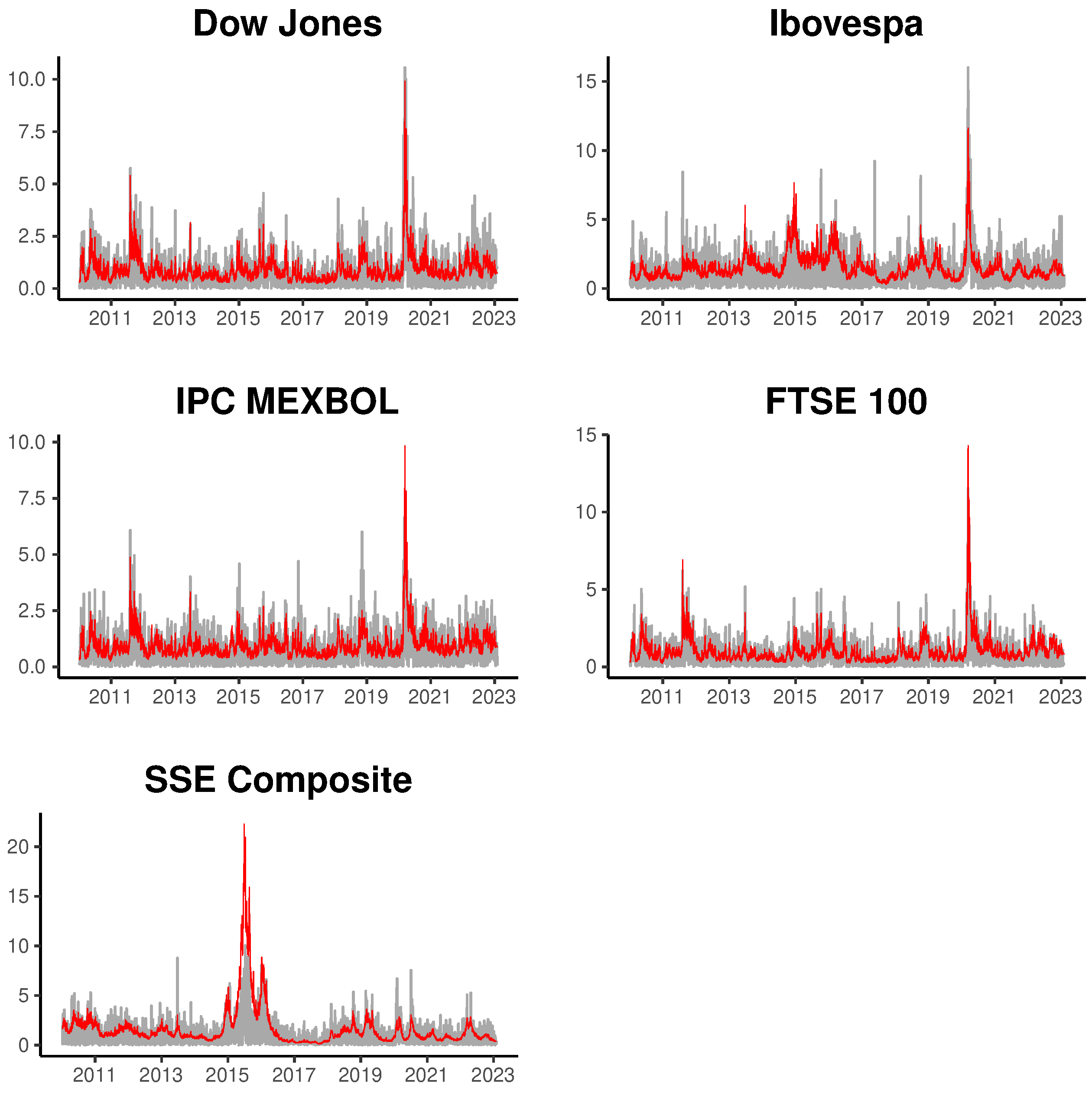
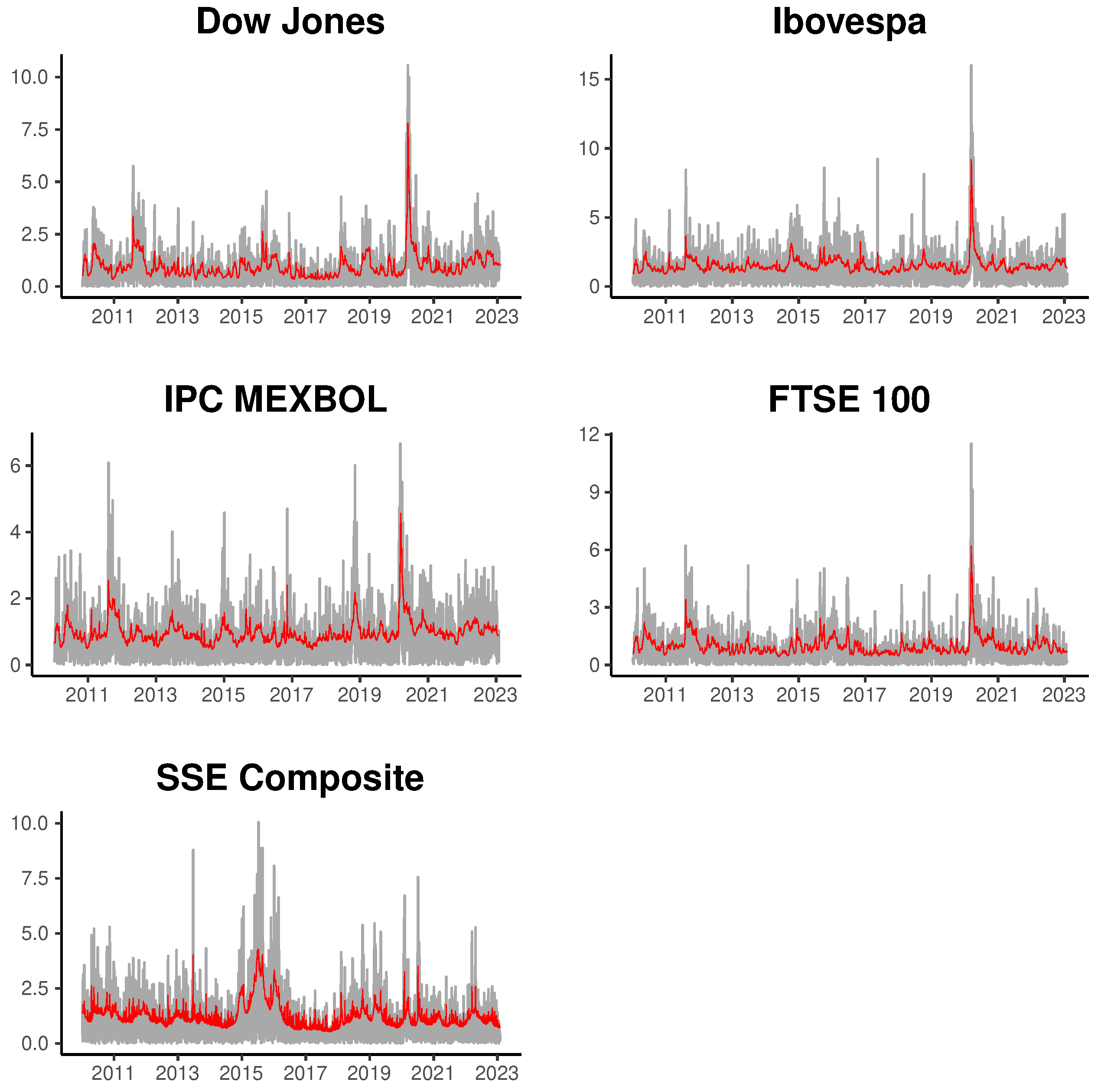
To illustrate the fit of the multifactor models, we present
Figure 2 and
Figure 3, displaying the estimated volatility for the four series using the most general models based on four latent factors. The gray line represents the absolute returns and the red lines the posterior mean of fitted volatilities for INLA and MCMC methods. In general, we can observe that the estimated volatility adequately tracks the movement in absolute returns, both in periods of low and high market volatility.
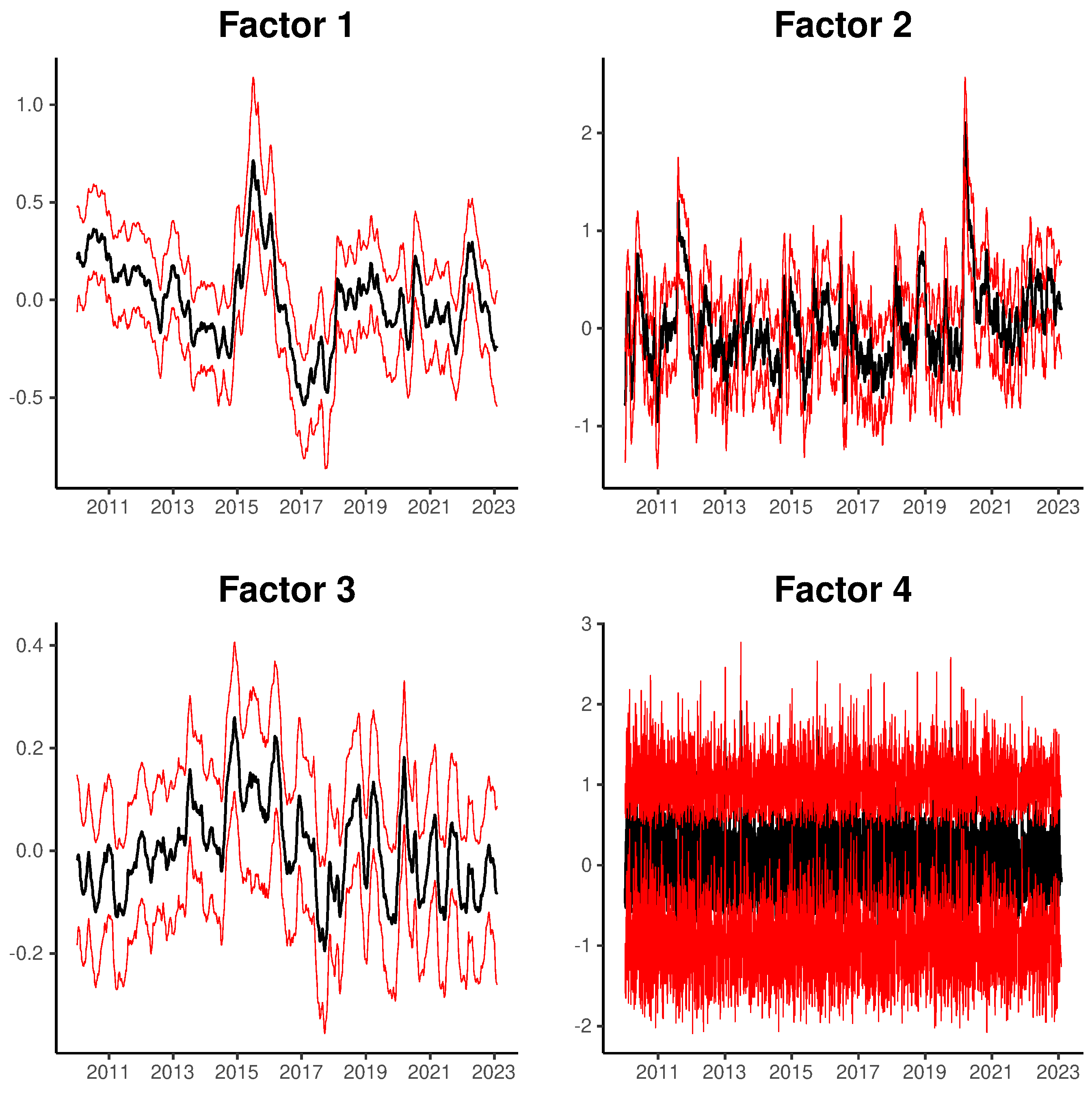
Finally, we illustrate the temporal evolution of the estimated latent factors in
Figure 4, which shows the posterior mean of the latent factors for the model with four latent factors (
Table 6), and a credibility interval of 95% constructed using the 2.5% and 97.5% percentiles of the posterior distribution of each latent factor. The black line represents the posterior mean and red lines the 2.5% and 97.5% percentiles of the credibility interval. We can note that the factors capture different persistence patterns, with factors 1, 2 and 3 associated with persistence values close to one in the autoregressive structure of the process, and factor four capturing shocks with almost zero persistence in the conditional volatility series.
4.3. Computational Cost
A relevant aspect to consider is the computational cost associated with each estimation.
Table 9 displays the elapsed time for estimation (in seconds) for each model for three sample sizes with 500, 1000 and 2714 observations, the last value corresponding to the sample of the analyzed data in the empirical section. Notably, INLA-based estimation demonstrates a significantly reduced computational cost compared to MCMC estimation using the algorithm and specification proposed by
Kastner et al. (
2017), especially for models with fewer latent factors.
In the larger sample size, for instance, for single-factor models, MCMC estimation takes 14.47 times longer than INLA estimation in the large sample analysis. However, this cost reduction becomes less pronounced for more complex models. In the case of models with four factors, the computational cost of MCMC estimation is approximately 3.84 times higher.
Comparing the sample sizes the computational cost of the INLA method appears to grow faster with an increasing number of factors compared to the MCMC-based method, but continues to be significantly lower in all analyses. It is essential to note that evaluating the effective cost of MCMC estimation in real situations can be more complex, as it depends on the convergence properties of the chains. In this experiment, we used chains of size 40,000, discarding the first 3500 samples. Still, for other models and sample sizes, the choice of the number of MCMC samples may differ.
The elapsed times were measured on a server with the following configuration: an Intel(R) Xeon(R) W-2265 processor with 24 threads running at 3.50 GHz and 128 GB of RAM memory. We used INLA version 23.09.09 (built on 9 September 2023). An important note is that we did not utilize the PARDISO sparse linear algebra library to speed up INLA calculations due to licensing restrictions at the time of writing the article.
4.4. Out-of-Sample Volatility Forecasting
To assess the predictive performance of the factor models of stochastic volatility, we conducted an out-of-sample forecast analysis, comparing the predictions of the factor models with one to four factors and the univariate stochastic volatility (SV)-based model estimated using INLA.
In this experiment, we generated out-of-sample predictions, forecasting one and five steps ahead, for the last 22 observations in our sample. We did this by employing a rolling sample approach, incrementing one observation at each step in the estimation sample. As with the in-sample analysis, we report the mean error (ME), root mean squared error (RMSE), and mean absolute error (MAE) between the predicted volatility values generated by each model and the absolute values of each series, serving as a proxy for true unobserved volatility, comparing the INLA and MCMC approaches.
Table 10 and
Table 11 provide a summary of the predictive results obtained in this analysis. For the one-step-ahead forecast (
Table 10), the results reveal a heterogeneous outcome regarding the best model for this horizon. For DJI, the three-factor model is favored, and for SSE, the four-factor model is chosen, both using the INLA approach. Remarkably, all three criteria consistently select the best model for each series. The specification based on univariate SV using INLA is chosen for IPC and LSE, while for BOV, the one-factor model estimated using MCMC is selected.
In the case of the five-step-ahead forecast horizon, as presented in
Table 11, the results suggest a better performance of more complex models, with the exception of the LSE and BOV series. Once again, the three criteria are consistent across all series, except for BOV. The INLA-based four-factor model is selected for DJI, and SSE, while the three-factor model using INLA is chosen for CPI. Conversely, the best model for LSE is based on a specification relying on univariate SV models using INLA, and for BOV the univariate models using MCMC are selected by the ME and MAE criteria, and the one-factor model using MCMC by the MSE criterion.
We finish the analysis of the predictive performance with a comparison of the predictive result for the multi-step forecasts for the last 22 observations in the sample without the use of rolling samples, comparing the predictive densities using the Log-Predictive Likelihood (
Gelman et al. 2014), again comparing the factor models proposed in the article with the formulation proposed by
Kastner et al. (
2017). In this analysis, we compared the predictive density for predictions 1, 5, 10 and 22 steps ahead, through the construction of the predictive log-likelihood obtained using the model predictions in a multivariate Gaussian distribution function. The advantages of this method are that it does not depend on any proxy for unobserved variance, and it allows evaluating predictions for all series simultaneously.
Table 12 show the results of this analysis.
In this analysis, we can observe that the predictive results were balanced between the two types of models, with the best result for 1-step and 10-steps ahead using INLA with one and three factors, and using MCMC for 5 and 22 steps ahead.
5. Conclusions
We introduce a multivariate extension to the class of stochastic volatility (SV) models estimated via Integrated Nested Laplace Approximations (INLA), incorporating a multifactor structure that enables a more parsimonious representation of this class of models. Our investigation focuses on the volatility dynamics of stock indexes.
We estimated the model using the log-returns of the Dow Jones Industrial, Ibovespa, Índice de Precios y Cotizaciones, FTSE 100, and SSE Composite Indexes. Subsequently, we assessed its performance in terms of accuracy and computational efficiency. Compared to the Markov Chain Monte Carlo (MCMC) approach, our results indicate that estimating multivariate SV models with INLA is feasible, with little to no compromise in terms of model fit quality. Additionally, there are significant time savings when using INLA to estimate the model parameters.
Regarding in-sample accuracy, our proposed formulation performed as well as or very close to its MCMC counterpart for nearly all assets and across various metrics. While there was no substantial difference in the numbers overall, it is worth noting that the MCMC estimation consistently outperformed the INLA-based approach for the Shanghai Chinese Stock Exchange Index (SSE). Nevertheless, INLA demonstrated a substantial reduction in estimation time, up to 14.47 times less than the MCMC alternative. This efficiency gap tends to decrease as more factors are introduced into the analysis.
We also conducted out-of-sample forecasting to evaluate the predictive performance of the factor stochastic volatility models. For the five-step-ahead forecast horizon, the more complex models (three and four-factor) consistently outperformed univariate models for each series, also estimated using INLA. However, for the one-step-ahead horizon, the univariate SV specification was preferred for the Índice de Precios y Cotizaciones (IPC) and FTSE 100 (LSE).
In conclusion, our work opens the door to further generalizations of the model, which could provide a deeper understanding of volatility patterns across a broader range of financial assets. Potential avenues include conducting Value at Risk (VaR) analyses and introducing additional specifications to better model the characteristics often attributed to financial time series, such as the presence of leverage effects and long memory processes. In the case of long memory processes, the analysis of intraday data may be particularly promising, as the large volume of observations should favor the use of methodologies like INLA over traditional MCMC-based approaches.
An interesting extension of our analysis would be a comparison of computational performance and predictive properties compared to estimations using Variational Bayes (
Gunawan et al. 2021;
Tan and Nott 2018), which also allows relevant computational gains in the Bayesian estimation of complex models. It is noteworthy that the recent implementation of the INLA methodology enables the incorporation of a Variational Bayes correction to the Gaussian approximation utilized in INLA for certain model classes, as discussed in
Van Niekerk et al. (
2023), thereby integrating the computational benefits of this method class into the use of Laplace approximations in Bayesian model estimation.


