
Is Monetary Policy a Driver of Cryptocurrencies? Evidence from a Structural Break GARCH-MIDAS Approach


Abstract
:1. Introduction
2. Materials and Methods
3. Results
4. Discussion
Author Contributions
Funding
Institutional Review Board Statement
Informed Consent Statement
Data Availability Statement
Conflicts of Interest
Abbreviations
| AIC | Akaike Information Criteria |
| AR | AutoRegressive |
| BIC | Bayesian Information Criteria |
| CBDCU | Central Bank Digital Currency Uncertainty Index |
| ECB | European Central Bank |
| EPU | Economic Policy Uncertainty |
| FRED | Federal Reserve Economic Data |
| GARCH | Generalized AutoRegressive Conditional Heteroskedasticity |
| MCS | Model Confidence Set |
| MDPI | Multidisciplinary Digital Publishing Institute |
| MIDAS | Mixed Data Sampling |
| MSE | Mean Squared Error |
| OMO | Open Market Operations |
| PoB | Proof-of-Burn |
| PoW | Proof-of-Work |
| QLIKE | Quasi-Likelihood |
| QLR | Quandt Likelihood Ratio |
| SB | Structural Break |
| SSM | Set of Superior Models |
| VAR | Vector AutoRegressive |
| VR | Variance Ratio |
| 1 | Alexakis et al. (2024) considered 93 events related to the limitation of fiat currency circulation. |
References
- Alexakis, Christos, Giulio Anselmi, and Giovanni Petrella. 2024. Flight to cryptos: Evidence on the use of cryptocurrencies in times of geopolitical tensions. International Review of Economics & Finance 89: 498–523. [Google Scholar] [CrossRef]
- Allaro, Hailegiorgis Bigramo, Belay Abera Kassa, and Bekele Hundie. 2018. A time series analysis of structural break time in the macroeconomic variables in Ethiopia. International Scholars Journals 6: 1–9. [Google Scholar]
- Amendola, Alessandra, Marinella Boccia, Vincenzo Candila, and Giampiero M. Gallo. 2020. Energy and non–energy commodities: Spillover effects on African stock markets. Journal of Statistical and Econometric Methods 9: 91–115. [Google Scholar] [CrossRef]
- Amendola, Alessandra, Vincenzo Candila, and Antonio Scognamillo. 2017. On the influence of US monetary policy on crude oil price volatility. Empirical Economics 52: 155–78. [Google Scholar] [CrossRef]
- Bai, Jushan, and Pierre Perron. 1998. Estimating and testing linear models with multiple structural changes. Econometrica 66: 47–78. [Google Scholar] [CrossRef]
- Baur, Dirk G., KiHoon Hong, and Adrian Lee. 2018. Bitcoin: Medium of exchange or speculative assets? Journal of International Financial Markets, Institutions and Money 54: 177–89. [Google Scholar] [CrossRef]
- Bollerslev, Tim. 1986. Generalized autoregressive conditional heteroskedasticity. Journal of Econometrics 31: 307–27. [Google Scholar] [CrossRef]
- Bundesbank, Deutsche. 2021. The Impact of the Eurosystem’s Monetary Policy on Bitcoin and Other Crypto Tokens. September. Available online: https://www.bundesbank.de/resource/blob/877282/6bd23da5a9b8ab8f472938b016628d39/mL/2021-09-geldpolitik-krypto-token-data.pdf (accessed on 1 June 2022).
- Candila, Vincenzo. 2021. Multivariate analysis of cryptocurrencies. Econometrics 9: 28. [Google Scholar] [CrossRef]
- Caton, James Lee. 2020. Cryptoliquidity: The blockchain and monetary stability. Journal of Entrepreneurship and Public Policy 9: 227–52. [Google Scholar] [CrossRef]
- Charfeddine, Lanouar, Noureddine Benlagha, and Youcef Maouchi. 2020. Investigating the dynamic relationship between cryptocurrencies and conventional assets: Implications for financial investors. Economic Modelling 85: 198–217. [Google Scholar] [CrossRef]
- Check, Adam, and Jeremy Piger. 2021. Structural breaks in U.S. macroeconomic time series: A bayesian model averaging approach. Journal of Money, Credit and Banking 53: 1999–2036. [Google Scholar] [CrossRef]
- Chen, James. 2020. What Is a M3? Definition, Liquidity, Disuse, and M Classifications. Available online: https://www.investopedia.com/terms/m/m3.asp (accessed on 1 June 2022).
- Chow, Gregory C. 1960. Tests of equality between sets of coefficients in two linear regressions. Econometrica 28: 591–605. [Google Scholar] [CrossRef]
- Conrad, Christian, and Onno Kleen. 2020. Two are better than one: Volatility forecasting using multiplicative component GARCH-MIDAS models. Journal of Applied Econometrics 35: 19–45. [Google Scholar] [CrossRef]
- Conrad, Christian, Anessa Custovic, and Eric Ghysels. 2018. Long- and short-term cryptocurrency volatility components: A GARCH-MIDAS analysis. Journal of Risk and Financial Management 11: 23. [Google Scholar] [CrossRef]
- Corbet, Shaen, Charles Larkin, Brian Lucey, Andrew Meegan, and Larisa Yarovaya. 2020. Cryptocurrency reaction to fomc announcements: Evidence of heterogeneity based on blockchain stack position. Journal of Financial Stability 46: 100706. [Google Scholar] [CrossRef]
- Corbet, Shaen, Grace McHugh, and Andrew Meegan. 2017. The influence of central bank monetary policy announcements on cryptocurrency return volatility. Investment Management and Financial Innovations 14: 60–72. [Google Scholar] [CrossRef]
- Demir, Ender, Giray Gözgör, Chi Keung Lau, and Samuel A. Vigne. 2018. Does economic policy uncertainty predict the bitcoin returns? An empirical investigation. Finance Research Letters 26: 145–49. [Google Scholar] [CrossRef]
- Dyhrberg, Anne Haubo. 2016. Hedging capabilities of bitcoin. Is it the virtual gold? Finance Research Letters 16: 139–44. [Google Scholar] [CrossRef]
- Engle, Robert F., and Tim Bollerslev. 1986. Modelling the persistence of conditional variances. Econometric Reviews 5: 1–50. [Google Scholar] [CrossRef]
- Engle, Robert F., Eric Ghysels, and Bumjean Sohn. 2013. Stock market volatility and macroeconomic fundamentals. The Review of Economics and Statistics 95: 776–97. [Google Scholar] [CrossRef]
- Éric Racicot, François, and Raymond Théoret. 2016. Macroeconomic shocks, forward-looking dynamics, and the behavior of hedge funds. Journal of Banking & Finance 62: 41–61. [Google Scholar] [CrossRef]
- Financial Stability Board (FSB). 2022. Assessment of Risks to Financial Stability from Crypto-Assets. Press Release, Crypto Assets to be Brought into South African Regulatory Purview. Available online: https://www.treasury.gov.za/comm_media/press/2021/IFWG_CAR%20WG_Position%20Paper%20on%20Crypto%20Assets_Press%20release_Final.pdf (accessed on 30 June 2021).
- Fletcher, Laurence. 2021. Hedge Funds Expect to Hold 7% of Assets in Crypto within Five Years. Available online: https://www.ft.com/content/4f8044bf-8f0f-46b4-9fb7-6d0eba723017#comments-anchor (accessed on 1 June 2022).
- Francis, Neville R., Laura E. Jackson, and Michael T. Owyang. 2020. How has empirical monetary policy analysis in the U.S. changed after the financial crisis? Economic Modelling 84: 309–21. [Google Scholar] [CrossRef]
- Glosten, Lawrence R., Ravi Jagannathan, and David E. Runkle. 1993. On the relation between the expected value and the volatility of the nominal excess return on stocks. The Journal of Finance 48: 1779–801. [Google Scholar] [CrossRef]
- Hansen, Peter R., Asger Lunde, and James M. Nason. 2011. The model confidence set. Econometrica 79: 453–97. [Google Scholar] [CrossRef]
- Hassani, Hossein, Xu Huang, and Emmanuel Silva. 2018. Banking with blockchain-ed big data. Journal of Management Analytics 5: 256–75. [Google Scholar] [CrossRef]
- Helmi, Mohamad Husam, Abdurrahman Nazif Çatık, and Coşkun Akdeniz. 2023. The impact of central bank digital currency news on the stock and cryptocurrency markets: Evidence from the TVP-VAR model. Research in International Business and Finance 65: 101968. [Google Scholar] [CrossRef]
- Inoue, Tomoo, and Tatsuyoshi Okimoto. 2008. Were there structural breaks in the effects of Japanese monetary policy? Re-evaluating policy effects of the lost decade. Journal of the Japanese and International Economies 22: 320–42. [Google Scholar] [CrossRef]
- Jiménez-Serranía, Vanessa, Javier Parra-Domínguez, Fernando De la Prieta, and Juan Manuel Corchado. 2022. Cryptocurrencies impact on financial markets: Some insights on its regulation and economic and accounting implications. In Blockchain and Applications. Edited by Javier Prieto, Alberto Partida, Paulo Leitão and António Pinto. Cham: Springer International Publishing, pp. 292–99. [Google Scholar]
- Karau, Sören. 2023. Monetary policy and bitcoin. Journal of International Money and Finance 137: 102880. [Google Scholar] [CrossRef]
- Koutmos, Dimitrios. 2018. Return and volatility spillovers among cryptocurrencies. Economics Letters 173: 122–27. [Google Scholar] [CrossRef]
- Lee, Dong Jin, and Jong Chil Son. 2013. Nonlinearity and structural breaks in monetary policy rules with stock prices. Economic Modelling 31: 1–11. [Google Scholar] [CrossRef]
- Li, Zhenghui, Bin Mo, and He Nie. 2023. Time and frequency dynamic connectedness between cryptocurrencies and financial assets in china. International Review of Economics & Finance 86: 46–57. [Google Scholar] [CrossRef]
- Ljung, G. M., and G. E. P. Box. 1978. On a measure of lack of fit in time series models. Biometrika 65: 297–303. [Google Scholar] [CrossRef]
- Lucarelli, Stefano, and Lucio Gobbi. 2023. Monetary policy in time of cryptocurrencies. In Reference Module in Social Sciences. Amsterdam: Elsevier. [Google Scholar] [CrossRef]
- Lucey, Brian M., Samuel A. Vigne, Larisa Yarovaya, and Yizhi Wang. 2022. The cryptocurrency uncertainty index. Finance Research Letters 45: 102147. [Google Scholar] [CrossRef]
- Ma, Chaoqun, Yonggang Tian, Shisong Hsiao, and Liurui Deng. 2022. Monetary policy shocks and bitcoin prices. Research in International Business and Finance 62: 101711. [Google Scholar] [CrossRef]
- Marmora, Paul. 2022. Does monetary policy fuel bitcoin demand? Event-study evidence from emerging markets. Journal of International Financial Markets, Institutions and Money 77: 101489. [Google Scholar] [CrossRef]
- Nekhili, Ramzi, Jahangir Sultan, and Elie Bouri. 2023. Liquidity spillovers between cryptocurrency and foreign exchange markets. The North American Journal of Economics and Finance 68: 101969. [Google Scholar] [CrossRef]
- Nguyen, Thai Vu Hong, Binh Thanh Nguyen, Kien Son Nguyen, and Huy Pham. 2019. Asymmetric monetary policy effects on cryptocurrency markets. Research in International Business and Finance 48: 335–39. [Google Scholar] [CrossRef]
- Owyang, Michael, and Howard Wall. 2004. Structural Breaks and Regional Disparities in the Transmission of Monetary Policy. (2003-008). FRB of St. Louis Working Paper No. 2003-008C. Available online: https://ssrn.com/abstract=927240 (accessed on 1 June 2022).
- Pan, Zhiyuan, Yudong Wang, Chongfeng Wu, and Libo Yin. 2017. Oil price volatility and macroeconomic fundamentals: A regime switching GARCH-MIDAS model. Journal of Empirical Finance 43: 130–42. [Google Scholar] [CrossRef]
- Perron, Pierre. 2005. Dealing with Structural Breaks. Working Papers Series WP2005-017; Boston: Department of Economics, Boston University. [Google Scholar]
- Quandt, Richard E. 1960. Tests of the hypothesis that a linear regression system obeys two separate regimes. Journal of the American Statistical Association 55: 324–30. [Google Scholar] [CrossRef]
- Saleh, Fahad. 2018. Volatility and Welfare in a Crypto Economy. SSRN Electronic Journal. [Google Scholar] [CrossRef]
- Seok, Sangik, Hoon Cho, Jennifer Eunkyeong Lee, and Doojin Ryu. 2023. Indirect effects of flow-performance sensitivity on fund performance. Borsa Istanbul Review 23: S1–S14. [Google Scholar] [CrossRef]
- Singh, Amitoj. 2022. South African Central Bank to Look at Regulating Crypto—coindesk.com. Available online: https://www.coindesk.com/policy/2022/07/13/south-african-central-bank-reverses-course-on-crypto-regulation/ (accessed on 9 September 2023).
- Štefan Lyócsa, Peter Molnár, Tomáš Plíhal, and Mária Širaňová. 2020. Impact of macroeconomic news, regulation and hacking exchange markets on the volatility of bitcoin. Journal of Economic Dynamics and Control 119: 103980. [Google Scholar] [CrossRef]
- Su, Zhi, Tong Fang, and Libo Yin. 2017. The role of news-based implied volatility among us financial markets. Economics Letters 157: 24–27. [Google Scholar] [CrossRef]
- Vidal-Tomás, David, and Ana Ibañez. 2018. Semi-strong efficiency of bitcoin. Finance Research Letters 27: 259–65. [Google Scholar] [CrossRef]
- Yang, Yang, Qing Liu, and Chia-Hsun Chang. 2023. China-Europe freight transportation under the first wave of COVID-19 pandemic and government restriction measures. Research in Transportation Economics 97: 101251. [Google Scholar] [CrossRef]
- Yen, Kuang-Chieh, Wei-Ying Nie, Hsuan-Ling Chang, and Li-Han Chang. 2023. Cryptocurrency return dependency and economic policy uncertainty. Finance Research Letters 56: 104182. [Google Scholar] [CrossRef]
- Yu, Miao. 2019. Forecasting bitcoin volatility: The role of leverage effect and uncertainty. Physica A: Statistical Mechanics and Its Applications 533: 120707. [Google Scholar] [CrossRef]
- Yu, Zhixiu. 2023. On the coexistence of cryptocurrency and fiat money. Review of Economic Dynamics 49: 147–80. [Google Scholar] [CrossRef]


| N.obs | Min | Mean | STD | Max | Kurtosis | Skewness | Time | |
|---|---|---|---|---|---|---|---|---|
| Cryptocurrency | ||||||||
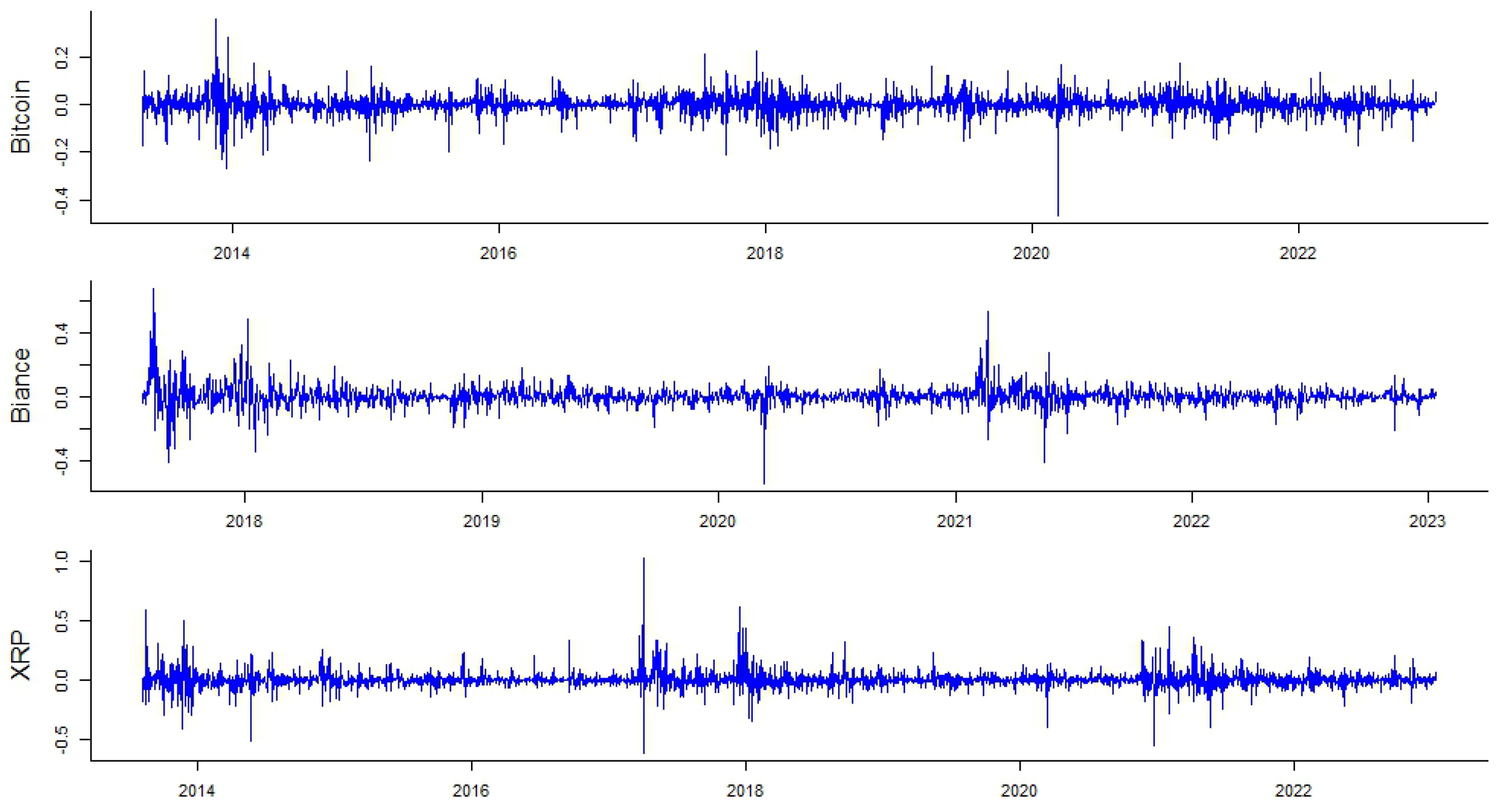
| Bitcoin | 3350 | −0.465 | 0.001 | 0.042 | 0.357 | 10.724 | −0.524 | April 2013–July 2022 |
| Binance Coin | 1801 | −0.543 | 0.004 | 0.070 | 0.675 | 15.025 | 0.915 | June 2017–July 2022 |
| XRP | 3252 | −0.616 | 0.001 | 0.071 | 1.027 | 26.791 | 1.577 | August 2013–July 2022 |
| Monetary Aggregate (M3) | ||||||||
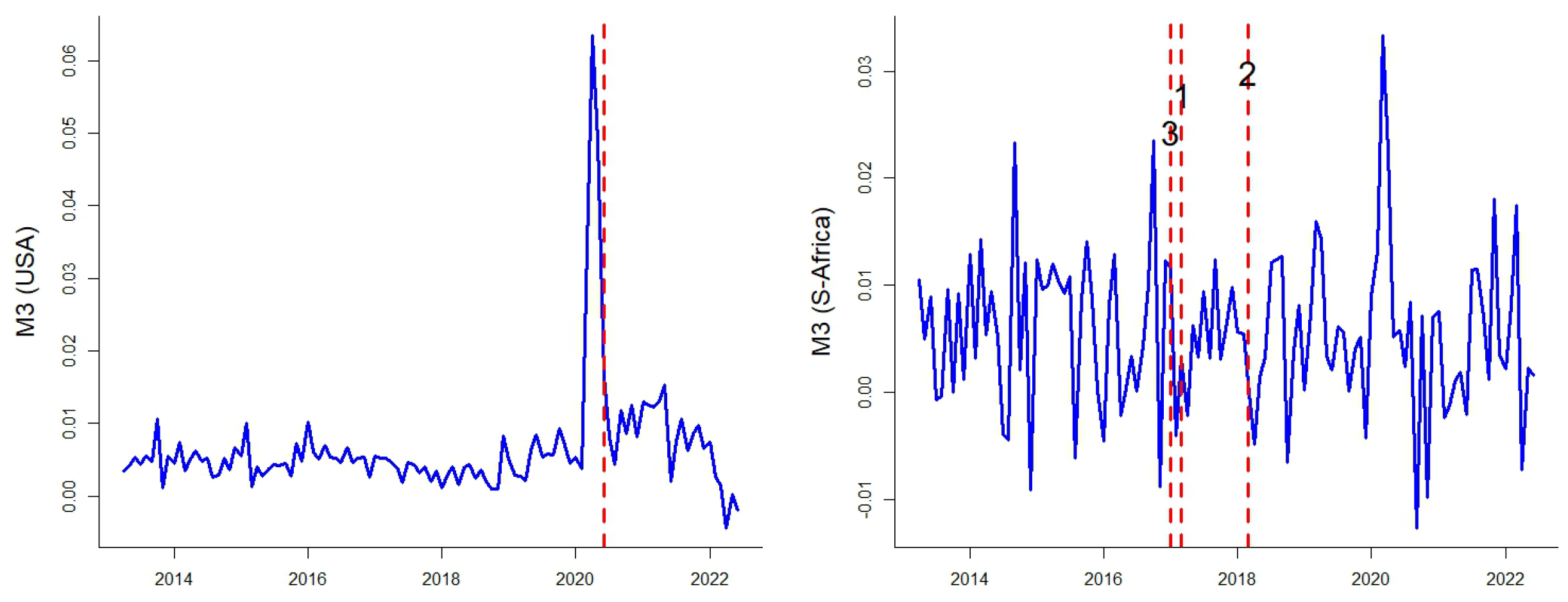
| USA | 111 | −0.004 | 0.007 | 0.008 | 0.063 | 27.918 | 4.856 | April 2013–July 2022 |
| S. Africa | 111 | −0.013 | 0.006 | 0.007 | 0.033 | 1.185 | 0.384 | April 2013–July 2022 |
| Panel A: The whole-sample evaluations. | |||||||
| GARCH | GJR | IGARCH | GM | SB-GM | GM | SB-GM | |
| M3(USA) | M3(USA) | M3(SA) | M3(SA) | ||||
| 0.000 | 0.000 | 0.000 *** | |||||
| (1.000) | (1.000) | (1.000) | |||||
| 0.127 *** | 0.132 *** | 0.127 *** | 0.131 *** | 0.155 *** | 0.133 *** | 0.203 *** | |
| (0.017) | (0.018) | (0.017) | (0.018) | (0.023) | (0.016) | (0.044) | |
| 0.018 ** | 0.085 *** | ||||||
| (0.008) | (0.015) | ||||||
| 0.872 *** | 0.875 *** | 0.873 | 0.878 *** | 0.853 *** | 0.875 *** | 0.819 *** | |
| (0.029) | (0.033) | (1.000) | (0.02) | (0.024) | (0.018) | (0.037) | |
| 0.988 *** | 0.916 *** | ||||||
| (0.013) | (0.02) | ||||||
| −0.017 | 3.24 *** | −0.022 | −0.02 | −0.019 | −0.048 | ||
| (0.025) | (0.124) | (0.018) | (0.024) | (0.019) | (0.036) | ||
| −0.014 | −0.01 | ||||||
| (0.014) | (0.021) | ||||||
| −4.418 *** | −4.238 *** | −4.49 *** | −4.344 *** | ||||
| (0.4) | (0.432) | (0.046) | (0.781) | ||||
| −5.24 *** | −4.704 *** | ||||||
| (0.491) | (0.305) | ||||||
| −25.274 *** | −25.973 *** | 2.646 *** | 42.375 *** | ||||
| (0.194) | (0.513) | (0.974) | (0.693) | ||||
| −94.428 *** | −88.306 *** | ||||||
| (0.516) | (14.865) | ||||||
| 3.714 *** | 1.776 *** | 2.034 ** | 6.576 *** | ||||
| (0.165) | (0.306) | (0.965) | (0.347) | ||||
| 1.099 *** | 1.396 ** | ||||||
| (0.267) | (0.704) | ||||||
| 3.25 *** | 3.255 *** | 3.284 *** | 3.194 *** | 3.268 *** | 2.947 *** | ||
| (0.16) | (0.166) | (0.126) | (0.124) | (0.122) | (0.133) | ||
| 3.493 *** | 3.408 *** | ||||||
| (0.516) | (0.218) | ||||||
| Panel B: Diagnostic tests for the whole sample. | |||||||
| AIC | −13,374.955 | −13,373.776 | −13,375.815 | −17,207.582 | −17,232.107 | −17,205.766 | −17,244.463 |
| BIC | −13,378.955 | −13,378.776 | −13,379.815 | −17,214.582 | −17,246.107 | −17,212.766 | −17,258.463 |
| MSE | 0.386 | 0.386 | 0.387 | 0.385 | 0.387 | 0.385 | 0.385 |
| QLIKE | −5.529 | −5.524 | −5.528 | −5.525 | −5.532 | −5.524 | −5.531 |
| LB | 0.865 | 0.878 | 0.866 | 0.877 | 0.896 | 0.868 | 0.943 |
| VR | 10.52 | 63.53 | 10.05 | 20.68 | |||
| Date of structural break in macro-variable (M3): | 31 May 2020 | 28 February 2017 | |||||
| [6.01] | [42.64] | ||||||
| Panel C: Diagnostic tests for period 1 (pre-break sample) according to the break date of M3 in the USA. | |||||||
| AIC | −10,425.467 | −10,423.924 | −10,426.135 | −13,387.073 | |||
| BIC | −10,429.467 | −10,428.924 | −10,430.135 | −13,394.073 | |||
| MSE | 0.476 | 0.475 | 0.477 | 0.475 | |||
| QLIKE | −5.509 | −5.505 | −5.509 | −5.506 | |||
| LB | 0.928 | 0.933 | 0.929 | 0.932 | |||
| Panel D: Diagnostic tests for period 2 (post-break sample) according to the break date of M3 in the USA. | |||||||
| AIC | −2962.947 | −2961.224 | −2963.075 | −3811.421 | |||
| BIC | −2966.947 | −2966.224 | −2967.075 | −3818.421 | |||
| MSE | 0.088 | 0.088 | 0.088 | 0.124 | |||
| QLIKE | −5.608 | −5.607 | −5.607 | −5.412 | |||
| LB | 0.714 | 0.776 | 0.719 | 0.551 | |||
| Panel E: Diagnostic tests for period 1 (pre-break sample) according to the break date of M3 in South Africa. | |||||||
| AIC | −5955.493 | −5954.629 | −5955.771 | −7562.956 | |||
| BIC | −5959.493 | −5959.629 | −5959.771 | −7569.956 | |||
| MSE | 0.389 | 0.392 | 0.39 | 0.395 | |||
| QLIKE | −5.72 | −5.718 | −5.721 | −5.724 | |||
| LB | 0.826 | 0.844 | 0.826 | 0.858 | |||
| Panel F: Diagnostic tests for period 2 (post-break sample) according to the break date of M3 in South Africa. | |||||||
| AIC | −7580.141 | −7578.36 | −7580.559 | −9834.627 | |||
| BIC | −7584.141 | −7583.36 | −7584.559 | −9841.627 | |||
| MSE | 0.377 | 0.376 | 0.377 | 0.373 | |||
| QLIKE | −5.414 | −5.409 | −5.412 | −5.387 | |||
| LB | 0.792 | 0.796 | 0.793 | 0.787 | |||
| Panel A: The whole-sample evaluations. | |||||||
| GARCH | GJR | IGARCH | GM | SB-GM | GM | SB-GM | |
| M3(USA) | M3(USA) | M3(SA) | M3(SA) | ||||
| 0.000 *** | 0.000 ** | 0.000 ** | |||||
| (1.000) | (1.000) | (1.000) | |||||
| 0.184 *** | 0.193 *** | 0.198 *** | 0.176 *** | 0.096 *** | 0.18 *** | 0.318 ** | |
| (0.048) | (0.052) | (0.053) | (0.054) | (0.032) | (0.048) | (0.136) | |
| 0.173 *** | 0.15 *** | ||||||
| (0.049) | (0.042) | ||||||
| 0.802 *** | 0.81 *** | 0.802 | 0.809 *** | 0.916 *** | 0.801 *** | 0.609 *** | |
| (0.044) | (0.049) | (1.000) | (0.065) | (0.032) | (0.059) | (0.191) | |
| 0.778 *** | 0.766 *** | ||||||
| (0.062) | (0.059) | ||||||
| −0.037 | 3.461 *** | −0.044 | −0.045 * | −0.037 | −0.124 | ||
| (0.041) | (0.242) | (0.033) | (0.027) | (0.035) | (0.148) | ||
| −0.03 | 0 | ||||||
| (0.05) | (0.039) | ||||||
| −5.115 *** | −4.998 *** | −5.073 *** | −4.067 *** | ||||
| (0.451) | (0.158) | (0.366) | (0.426) | ||||
| −5.456 *** | −5.445 *** | ||||||
| (0.394) | (0.248) | ||||||
| −22.352 ** | −17.43 *** | −39.769 *** | −2.589 * | ||||
| (10.534) | (5.146) | (0.153) | (1.481) | ||||
| −27.996 *** | −52.299 *** | ||||||
| (9.185) | (14.808) | ||||||
| 5.609 *** | 11.84 | 1.981 *** | 1.786 *** | ||||
| (0.499) | (66.736) | (0.495) | (0.606) | ||||
| 5.707 *** | 1.883 *** | ||||||
| (0.814) | (0.395) | ||||||
| 3.593 *** | 3.601 *** | 3.79 *** | 3.512 *** | 3.793 *** | 4.209 *** | ||
| (0.341) | (0.343) | (0.382) | (0.246) | (0.289) | (1.011) | ||
| 4.295 *** | 3.775 *** | ||||||
| (0.559) | (0.342) | ||||||
| Panel B: Diagnostic tests for the whole sample. | |||||||
| AIC | −5613.859 | −5612.757 | −5613.511 | −7676.302 | −7667.471 | −7672.958 | −7676.942 |
| BIC | −5617.859 | −5617.757 | −5617.511 | −7683.302 | −7681.471 | −7679.958 | −7690.942 |
| MSE | 3.676 | 3.68 | 3.727 | 3.624 | 3.67 | 3.623 | 3.58 |
| QLIKE | −4.791 | −4.789 | −4.788 | −4.796 | −4.783 | −4.792 | −4.804 |
| LB | 0.229 | 0.183 | 0.24 | 0.225 | 0.119 | 0.164 | 0.092 |
| VR | 7.18 | 10.29 | 6.73 | 20.59 | |||
| Date of structural break in macro-variable (M3): | 31 May 2020 | 28 February 2018 | |||||
| [24.62] | [8.68] | ||||||
| Panel C: Diagnostic tests for period 1 (pre-break sample) according to the Break date of M3 in the USA. | |||||||
| AIC | −3089.287 | −3089.156 | −3089.325 | −4277.974 | |||
| BIC | −3093.287 | −3094.156 | −3093.325 | −4284.974 | |||
| MSE | 5.096 | 5.16 | 5.101 | 5.078 | |||
| QLIKE | −4.62 | −4.605 | −4.62 | −4.604 | |||
| LB | 0.161 | 0.112 | 0.161 | 0.123 | |||
| Panel D: Diagnostic tests for period 2 (post-break sample) according to the break date of M3 in the USA. | |||||||
| AIC | −2644.687 | −2642.8 | −2642.594 | −3551.629 | |||
| BIC | −2648.687 | −2647.8 | −2646.594 | −3558.629 | |||
| MSE | 1.686 | 1.685 | 1.754 | 1.672 | |||
| QLIKE | −5.05 | −5.05 | −5.043 | −5.058 | |||
| LB | 0.646 | 0.651 | 0.66 | 0.694 | |||
| Panel E: Diagnostic tests for period 1 (pre-break sample) according to the break date of M3 in South Africa. | |||||||
| AIC | −323.15 | −313.887 | −323.148 | −566.227 | |||
| BIC | −327.15 | −318.887 | −327.148 | −573.227 | |||
| MSE | 20.359 | 19.301 | 20.528 | 18.585 | |||
| QLIKE | −3.202 | −3.237 | −3.201 | −3.217 | |||
| LB | 0.82 | 0.015 | 0.824 | 0.831 | |||
| Panel F: Diagnostic tests for period 2 (post-break sample) according to the break date of M3 in South Africa. | |||||||
| AIC | −5344.646 | −5342.673 | −5340.995 | −7189.583 | |||
| BIC | −5348.646 | −5347.673 | −5344.995 | −7196.583 | |||
| MSE | 1.531 | 1.532 | 1.595 | 1.61 | |||
| QLIKE | −4.992 | −4.993 | −4.98 | −4.982 | |||
| LB | 0.052 | 0.051 | 0.056 | 0.049 | |||
| Panel A: The whole-sample evaluations. | |||||||
| GARCH | GJR | IGARCH | GM | SB-GM | GM | SB-GM | |
| M3(USA) | M3(USA) | M3(SA) | M3(SA) | ||||
| 0.000 * | 0.000 * | 0.000 *** | |||||
| (1.000) | (1.000) | (1.000) | |||||
| 0.236 *** | 0.25 *** | 0.236 *** | 0.251 *** | 0.318 *** | 0.247 *** | 0.384 *** | |
| (0.048) | (0.062) | (0.05) | (0.06) | (0.101) | (0.061) | (0.131) | |
| 0.143 ** | 0.227 *** | ||||||
| (0.071) | (0.079) | ||||||
| 0.763 *** | 0.761 *** | 0.764 | 0.76 *** | 0.702 *** | 0.761 *** | 0.65 *** | |
| (0.067) | (0.069) | (1.000) | (0.052) | (0.086) | (0.054) | (0.099) | |
| 0.857 *** | 0.764 *** | ||||||
| (0.099) | (0.083) | ||||||
| −0.025 | 2.982 *** | −0.031 | −0.049 | −0.026 | −0.079 | ||
| (0.042) | (0.096) | (0.037) | (0.053) | (0.034) | (0.091) | ||
| −0.049 | −0.025 | ||||||
| (0.043) | (0.041) | ||||||
| −3.133 *** | −2.783 *** | −3.232 *** | −3.609 *** | ||||
| (0.245) | (0.294) | (0.279) | (0.206) | ||||
| −4.339 *** | −3.96 *** | ||||||
| (0.511) | (0.423) | ||||||
| −19.636 *** | −16.924 *** | −7.302 | 10.942 *** | ||||
| (1.558) | (1.453) | (5.626) | (4.131) | ||||
| −68.777 *** | −89.538 *** | ||||||
| (1.427) | (2.3) | ||||||
| 5.818 | 3.058 ** | 2.235 *** | 2.013 *** | ||||
| (20.956) | (1.346) | (0.142) | (0.263) | ||||
| 1.715 | 1.001 *** | ||||||
| (1.214) | (0.197) | ||||||
| 2.986 *** | 2.987 *** | 2.99 *** | 2.967 *** | 3.001 *** | 3.177 *** | ||
| (0.123) | (0.127) | (0.156) | (0.112) | (0.099) | (0.194) | ||
| 3.141 *** | 2.925 *** | ||||||
| (0.233) | (0.118) | ||||||
| Panel B: Diagnostic tests for the whole sample. | |||||||
| AIC | −10,763.666 | −10,762.17 | −10,764.031 | −14,484.743 | −14,490.27 | −14,480.541 | −14,490.22 |
| BIC | −10,767.666 | −10,767.17 | −10,768.031 | −14,491.743 | −14,504.27 | −14,487.541 | −14,504.22 |
| MSE | 7.202 | 7.229 | 7.209 | 7.221 | 7.308 | 7.209 | 7.162 |
| QLIKE | −4.773 | −4.775 | −4.773 | −4.782 | −4.781 | −4.778 | −4.769 |
| LB | 0.872 | 0.866 | 0.872 | 0.831 | 0.826 | 0.851 | 0.887 |
| VR | 0.72 | 23.15 | 0.23 | 6.71 | |||
| Date of structural break in macro-variable (M3): | 31 May 2020 | 31 December 2016 | |||||
| [6.09] | [37.08] | ||||||
| Panel C: Diagnostic tests for period 1 (pre-break sample) according to the break date of M3 in the USA. | |||||||
| AIC | −8376.714 | −8375.693 | −8376.979 | −11,226.149 | |||
| BIC | −8380.714 | −8380.693 | −8380.979 | −11,233.149 | |||
| MSE | 8.498 | 8.578 | 8.505 | 8.578 | |||
| QLIKE | −4.806 | −4.81 | −4.806 | −4.814 | |||
| LB | 0.874 | 0.866 | 0.875 | 0.842 | |||
| Panel D: Diagnostic tests for period 2 (post-break sample) according to the break date of M3 in the USA. | |||||||
| AIC | −2533.104 | −2531.254 | −2533.183 | −3445.654 | |||
| BIC | −2537.104 | −2536.254 | −2537.183 | −3452.654 | |||
| MSE | 3.1 | 3.095 | 3.103 | 3.013 | |||
| QLIKE | −4.711 | −4.715 | −4.711 | −4.743 | |||
| LB | 0.886 | 0.883 | 0.886 | 0.655 | |||
| Panel E: Diagnostic tests for period 1 (pre-break sample) according to the break date of M3 in South Africa. | |||||||
| AIC | −4334.846 | −4333.954 | −4335.009 | −5756.526 | |||
| BIC | −4338.846 | −4338.954 | −4339.009 | −5763.526 | |||
| MSE | 3.51 | 3.599 | 3.513 | 3.591 | |||
| QLIKE | −4.824 | −4.835 | −4.824 | −4.829 | |||
| LB | 0.96 | 0.955 | 0.96 | 0.958 | |||
| Panel F: Diagnostic tests for period 2 (post-break sample) according to the break date of M3 in South Africa. | |||||||
| AIC | −6590.052 | −6588.334 | −6590.254 | −8922.088 | |||
| BIC | −6594.052 | −6593.334 | −6594.254 | −8929.088 | |||
| MSE | 9.378 | 9.397 | 9.387 | 9.203 | |||
| QLIKE | −4.736 | −4.738 | −4.736 | −4.758 | |||
| LB | 0.876 | 0.887 | 0.876 | 0.901 | |||
Disclaimer/Publisher’s Note: The statements, opinions and data contained in all publications are solely those of the individual author(s) and contributor(s) and not of MDPI and/or the editor(s). MDPI and/or the editor(s) disclaim responsibility for any injury to people or property resulting from any ideas, methods, instructions or products referred to in the content. |
© 2024 by the authors. Licensee MDPI, Basel, Switzerland. This article is an open access article distributed under the terms and conditions of the Creative Commons Attribution (CC BY) license (https://creativecommons.org/licenses/by/4.0/).
Share and Cite
Alam, M.S.; Amendola, A.; Candila, V.; Jabarabadi, S.D. Is Monetary Policy a Driver of Cryptocurrencies? Evidence from a Structural Break GARCH-MIDAS Approach. Econometrics 2024, 12, 2. https://doi.org/10.3390/econometrics12010002
Alam MS, Amendola A, Candila V, Jabarabadi SD. Is Monetary Policy a Driver of Cryptocurrencies? Evidence from a Structural Break GARCH-MIDAS Approach. Econometrics. 2024; 12(1):2. https://doi.org/10.3390/econometrics12010002
Chicago/Turabian StyleAlam, Md Samsul, Alessandra Amendola, Vincenzo Candila, and Shahram Dehghan Jabarabadi. 2024. "Is Monetary Policy a Driver of Cryptocurrencies? Evidence from a Structural Break GARCH-MIDAS Approach" Econometrics 12, no. 1: 2. https://doi.org/10.3390/econometrics12010002