Article

Detecting Pump-and-Dumps with Crypto-Assets: Dealing with Imbalanced Datasets and Insiders’ Anticipated Purchases

by
Dean Fantazzini
1,2,*,† and
Yufeng Xiao
1,†
1
Moscow School of Economics, Moscow State University, 119992 Moscow, Russia
2
Faculty of Economic Sciences, Higher School of Economics, 109028 Moscow, Russia
*
Author to whom correspondence should be addressed.
These authors contributed equally to this work.
Econometrics 2023, 11(3), 22; https://doi.org/10.3390/econometrics11030022
Submission received: 11 May 2023 / Revised: 20 July 2023 / Accepted: 21 August 2023 / Published: 30 August 2023

Abstract

:
Detecting pump-and-dump schemes involving cryptoassets with high-frequency data is challenging due to imbalanced datasets and the early occurrence of unusual trading volumes. To address these issues, we propose constructing synthetic balanced datasets using resampling methods and flagging a pump-and-dump from the moment of public announcement up to 60 min beforehand. We validated our proposals using data from Pumpolymp and the CryptoCurrency eXchange Trading Library to identify 351 pump signals relative to the Binance crypto exchange in 2021 and 2022. We found that the most effective approach was using the original imbalanced dataset with pump-and-dumps flagged 60 min in advance, together with a random forest model with data segmented into 30-s chunks and regressors computed with a moving window of 1 h. Our analysis revealed that a better balance between sensitivity and specificity could be achieved by simply selecting an appropriate probability threshold, such as setting the threshold close to the observed prevalence in the original dataset. Resampling methods were useful in some cases, but threshold-independent measures were not affected. Moreover, detecting pump-and-dumps in real-time involves high-dimensional data, and the use of resampling methods to build synthetic datasets can be time-consuming, making them less practical.

1. Introduction

A cryptocurrency is a form of digital currency that uses strong encryption and a ledger for protection. It allows users to buy goods and services online and is usually traded for speculative purposes. Blockchain technology is the backbone of a cryptocurrency, enabling it to function through a decentralized, distributed system that records transactions on multiple computers; see Antonopoulos (2014), Narayanan et al. (2016) for a technical discussion at the textbook level. At the time of writing this paper, there were over 10,000 publicly traded cryptocurrencies, with a total market value exceeding USD 2.2 trillion as of 1 March 2022, according to CoinMarketCap.com, accessed on 1 December 2022.
The unregulated nature of the cryptocurrency market has led to the emergence of pump-and-dump schemes, a traditional form of securities fraud. Fraudsters use social media platforms such as Telegram, Discord, and Twitter to initially spread false information and manipulate the price of low market-cap crypto assets. They then sell their holdings to make a profit, causing the price to fall and investors to lose money.
Kamps and Kleinberg (2018) and La Morgia et al. (2020, 2023) examined large sets of pumps-and-dumps and proposed several market-based approaches to detect them. Unfortunately, the detection of pump-and-dumps with crypto assets and high-frequency data involves imbalanced datasets where the minority class flagging the pump-and-dumps is very small (usually less than 0.2% of all cases). Moreover, even if the VIP members of the social media groups organizing these market manipulations are supposed to receive detailed information about them seconds or minutes before the general public (and they pay a fee for such a service), in reality, unusual trading volumes can take place much earlier. These two problems can strongly affect the performance of any classifier used to flag potential pump-and-dump activity.
This study aims to solve these issues by building synthetic balanced datasets and enlarging the time sample flagging a pump-and-dump. The goal is to make it easier for investors to make informed decisions, and for financial regulators to prevent fraudulent activities in the cryptocurrency market.
To reach the paper’s objective, we built synthetic balanced datasets generated according to four remedies for class imbalances proposed in the statistical literature. Moreover, we flagged a pump-and-dump from the minute of the public announcement up to 60 min before it. This simple solution was able to both deal with the insiders’ anticipated purchases of the targeted crypto-assets and to solve the issue of imbalanced datasets. An empirical analysis with 351 pump-and-dumps that took place in 2021–2022 and a set of machine learning methods to detect these illegal activities confirmed the validity of the proposed solutions.
The paper is organized as follows: Section 2 reviews the literature devoted to cryptocurrency price manipulation and pump-and-dumps, while the methods proposed to detect pump-and-dump schemes are discussed in Section 3. The empirical results are reported in Section 4, while robustness checks are discussed in Section 5. Section 6 briefly concludes.

2. Literature Review

2.1. Pump-and-Dumps

In the last two decades, the financial literature has extensively examined “pump-and-dump” schemes, which are fraudulent practices involving the artificial inflation of stock prices through deceptive statements. These schemes aim to sell overvalued securities for a profit, leaving unsuspecting buyers with worthless investments. Researchers have focused on understanding the mechanics of these schemes, their impact on small retail investors, market efficiency, and the role of regulators in prevention.
Zaki et al. (2012) present a case study and propose architectural solutions to detect and prevent “pump-and-dump” schemes. They use simulations to demonstrate the manipulation’s effects on market stability and investor confidence.
Withanawasam et al. (2013) develop a framework for market manipulation, specifically in a limit-order market. They show that “pump-and-dump” manipulation becomes profitable in the presence of technical traders, who exploit information asymmetry and generate profits by raising prices and selling immediately.
Bouraoui (2015) analyzes the impact of stock spam on stock prices and investor behavior. Despite investors’ awareness of scams, the study finds that stock prices increase due to information asymmetry and the influence of spammers.
Siering (2019) examine the economics of “pump-and-dump” schemes in internet-based stock promotion. They analyze the schemes’ financial and organizational structures, participants’ incentives, and their effects on stock prices and investor behavior. The article emphasizes the need for increased regulation to protect investors and maintain market stability.
Ouyang and Cao (2020) investigate pump-and-dump events in the Chinese stock market. They find that smaller, less liquid stocks are more vulnerable to manipulation, and indicators such as market capitalization, free float, and liquidity provide insights into manipulators’ allocation strategies.
Additionally, several academic and professional surveys provide general introductions to pump-and-dump schemes in financial markets; see US Security and Exchange Commission (2005), Krinklebine (2010), and Frieder and Zittrain (2008).

2.2. Cryptocurrency Pump-and-Dumps

The surge of cryptocurrencies in an unregulated environment has raised concerns about fraudulent activities, leading to a growing body of literature investigating pump-and-dump schemes in the cryptocurrency market. These schemes involve coordinated efforts to inflate the price of a specific cryptocurrency for personal profit. Social media platforms such as Telegram and Discord have been identified as common platforms for these schemes. Studies have explored the factors influencing the success of pump-and-dump schemes, the effectiveness of machine learning models in detecting and predicting these schemes, and the impact of such schemes on the cryptocurrency market.
Feder et al. (2018) examined pump-and-dump schemes on Telegram and Discord, identifying factors such as low market capitalization and liquidity that make certain cryptocurrencies more susceptible to targeting by pump groups. Similarly, Dhawan and Putniņš (2023) highlighted the correlation between low liquidity and higher abnormal returns in cryptocurrencies, indicating the significance of liquidity in these schemes. Victor and Hagemann (2019) compared pump-and-dump schemes in the cryptocurrency market to penny stock schemes and proposed the use of machine learning for detection.
Xu and Livshits (2019) investigated pump-and-dump events in cryptocurrencies, analyzing the fake trading volume and high profits obtained by organizers. Their machine learning models accurately predicted pump likelihoods, yielding significant returns. Using a similar approach, Shao (2021) employed several supervised learning models, including random forests, decision trees, and k-nearest neighbors, to detect pump-and-dump schemes in Dogecoin, with the random forest model being the most effective.
Hamrick et al. (2021) monitored Telegram channels and observed short-term price increases resulting from pump campaigns, but noted a decline in impact over time. They differentiated between transparent pumps, which provided clear information such as the coin name and target profit, and “obscure” pumps, which only hinted at potential price increases. The results showed that transparent pumps generated higher returns than obscure pumps. Nghiem et al. (2021) proposed a method using market and social media signals to predict target cryptocurrencies for pump-and-dump schemes, achieving superior results compared to existing methods.
Kamps and Kleinberg (2018) developed a machine learning model trained on pump-and-dump event data to effectively detect these schemes. Based on this analysis, La Morgia et al. (2020) conducted an in-depth examination of community-organized pumps and dumps, reporting several case studies and providing a real-time detection classifier for investors that outperformed all the other competing models. La Morgia et al. (2023) extended this work by introducing an AdaBoost classifier, which achieved better precision, recall, and F1-score results.
Overall, these studies contribute to the understanding of pump-and-dump schemes in the cryptocurrency market, provide insights into detection techniques, and emphasize the need for regulation to mitigate financial harm to investors.

2.3. The Class Imbalance Problem

The class imbalance problem is a significant challenge in classification tasks. Neglecting class imbalance can lead to severe implications for model estimation and accuracy evaluation; see the reviews by He and Garcia (2009) and Sun et al. (2009) for more in-depth discussions. Different classification methods exhibit various behaviors in the presence of class imbalance. For example, logistic regression underestimates conditional probabilities of the rare class King and Zeng (2001) and linear discriminant analysis is also affected by imbalanced class distributions Hand and Vinciotti (2003). Moreover, nonparametric methods tend to favor classification rules that perform well only on the frequent class Chawla (2003), Akbani et al. (2004), Cieslak and Chawla (2008).
Research on imbalanced classification focuses on two main approaches: learning level solutions and data level solutions Kotsiantis et al. (2006). Learning level solutions aim to enhance the learning process for the minority class by modifying the classifier or adjusting misclassification costs Riddle et al. (1994), Cieslak and Chawla (2008), Breiman et al. (1984), Ting (2002), Kukar and Kononenko (1998), Lin et al. (2002). However, cost information is often unavailable.
Data level solutions focus on altering the class distribution to obtain a more balanced sample, but methods such as Random Over-Sampling and Random Under-Sampling have drawbacks such as loss of important data, decrease in sample size, increased risk of overfitting, and additional computational effort McCarthy et al. (2005).
Recent works propose generating artificial examples similar to the observations in the minority class to reduce overfitting and improve generalization Lee (1999), Chawla et al. (2002), Guo and Viktor (2004), Mease et al. (2007), Menardi and Torelli (2014), and Lunardon et al. (2014).
The accuracy evaluation of classifiers is equally important in class imbalance settings Weiss and Provost (2001) and Weiss (2004). Common performance measures such as error rate can be misleading due to their dependence on class distribution. Precision, recall, F-measure, receiver operating characteristic (ROC) curve, precision-recall curves, and cost curves are more suitable for evaluation He and Garcia (2009).
Estimating the accuracy measure is challenging in imbalanced learning when there are few examples of the rare class. Common error estimators include apparent error, holdout method, bootstrapping, and cross-validation techniques. However, in strongly imbalanced frameworks, evaluating results on the same data used in training or on a test sample may lead to high variance estimates and scarcity of rare examples Menardi and Torelli (2014), Schiavo and Hand (2000).

3. Materials and Methods

Detecting pump-and-dump schemes in the cryptocurrency market using high-frequency data is a challenging task. This is because such schemes are often associated with imbalanced datasets, where the instances of pump-and-dump cases are very rare, usually comprising less than 0.2% of all cases. Additionally, it is widely assumed that members of social media groups that organize these market manipulations are given detailed information about the scheme seconds or minutes before it is made public; see Kamps and Kleinberg (2018) and La Morgia et al. (2020, 2023). They pay a fee for such advanced knowledge, but in reality, unusual trading volumes can occur much earlier than that, complicating the process of detecting such schemes. These two problems can significantly impact the performance of any machine learning classifier used for detecting pump-and-dump activities, making it difficult to accurately identify such instances in a timely manner.
We will first provide a brief review of the four methods used to address class imbalance in our empirical analysis. In addition, we will present a simple solution to increase the dimensionality of the minority class, which involves flagging instances of pump-and-dump schemes from the moment of public announcement up to 60 min prior to it. Subsequently, we will discuss classification models that are capable of detecting pump-and-dump schemes.

3.1. Building Synthetic Balanced Datasets

Resolving class imbalance is crucial for accurate prediction models in binary outcomes. Popular resampling techniques include Random Under-Sampling (RUS), Random Over-Sampling (ROS), the Synthetic Minority Over-sampling Technique (SMOTE) by Chawla et al. (2002), and the Random Over-Sampling Examples (ROSE) by Menardi and Torelli (2014).
The RUS method reduces the majority class by randomly sampling from it until it matches the number of minority class samples. The ROS method replicates minority class observations to achieve balance. SMOTE generates synthetic minority class observations by interpolating between existing observations and their nearest neighbors. ROSE combines over-sampling and under-sampling by resampling the majority and minority classes using bootstrap techniques, followed by generating synthetic samples in the feature space neighborhood Menardi and Torelli (2014).
RUS can be effective when the dataset is large, but may lose information in small datasets or if the minority class contains important information. ROS works well for small datasets but may not handle outliers or noisy data. SMOTE is effective for small datasets with proximity between minority and majority classes, but it may struggle if the minority class is sparse or if there is high overlap between the minority and majority classes in the feature space. Moreover, the choice of the number of k nearest minority class neighbors in SMOTE impacts its effectiveness. ROSE generates synthetic samples representative of the minority class and is useful for extreme imbalanced learning Menardi and Torelli (2014). The detailed description of all these resampling methods is reported in Appendix A.
The previous four methods have been shown to effectively balance the data distribution and improve model performance in several cases, enabling more precise classification of individuals into high and low risk groups. However, more recent research has revealed mixed results and has highlighted potential drawbacks associated with these resampling methods. In certain cases, these methods may even lead to a decline in model performance and wrong model interpretations; see Tantithamthavorn et al. (2018), Wongvorachan et al. (2023), and van den Goorbergh et al. (2022).
Given the potential challenges associated with the methods used to address class imbalance, we propose a simple approach to increasing the size of the minority class in the context of our dataset, which deals with pump-and-dump schemes involving crypto-assets. Prior research has suggested that paying VIP members of the social media groups involved in such market manipulations receive detailed information about them seconds or minutes before the general public; see, for example, Kamps and Kleinberg (2018) and La Morgia et al. (2020, 2023), and references therein. However, upon analyzing our dataset, we discovered that unusual trading volumes can occur much earlier, particularly within 60 min prior to the public announcement (see Figure A3, Figure A4, Figure A5, Figure A6, Figure A7, Figure A8, Figure A9, Figure A10, Figure A11, Figure A12, Figure A13, Figure A14, Figure A15, Figure A16, Figure A17, Figure A18, Figure A19, Figure A20, Figure A21, Figure A22, Figure A23, Figure A24, Figure A25, Figure A26, Figure A27, Figure A28, Figure A29, Figure A30, Figure A31, Figure A32, Figure A33, Figure A34, Figure A35, Figure A36, Figure A37, Figure A38, Figure A39, Figure A40, Figure A41, Figure A42, Figure A43, Figure A44, Figure A45 and Figure A46 in Appendix D). These atypical trades are likely executed by the true organizers of the pump-and-dump, who are likely the only ones profiting from these manipulations. As a result, we propose flagging a pump-and-dump from the minute of the public announcement up to 60 min before it, rather than only 1 or 2 min prior to it, as has been done in the past. This straightforward solution has the potential to address both insider anticipated purchases of the targeted crypto-assets and the issue of imbalanced datasets. In addition to the time frame of up to 60 min before the public announcement, we also experimented with longer time frames, such as up to 24 h before the announcement. However, the performance metrics obtained from these longer time frames were worse, and hence were not included in this study.

3.2. Methods for Binary Classification: A (Brief) Review

We employed three different classifiers, namely the logit model, random forests, and AdaBoost, to detect the onset of fraudulent pump-and-dump schemes. These classifiers have previously been used in La Morgia et al. (2020, 2023) and have demonstrated superior performance in detecting such schemes compared to previous state-of-the-art models. We present a brief overview of these models below, while a more comprehensive discussion at the textbook level can be found in Hastie et al. (2017).
The logit model can be expressed as follows,
P ( Y = 1 | X ) = exp ( β 0 + β 1 X 1 + + β p X p ) / ( 1 + exp ( β 0 + β 1 X 1 + + β p X p ) )
where P ( Y = 1 | X ) is the probability of Y being 1 given the predictor variables X , β 0 is the intercept, β 1 , …, β p are the parameters associated with each predictor variable, and X 1 , …, X p are the predictor variables. In our case, Y = 1 denotes the presence of a pump-and-dump scheme.
Random forests are an ensemble learning method that combines multiple decision trees to make a prediction. In a random forest model, multiple decision trees are constructed using bootstrap samples of the training data and a random subset of the predictor variables. The final prediction is made by aggregating the predictions of all the individual trees. The randomness in the tree-building process and the use of multiple trees help to reduce the overfitting problem and improve the model’s accuracy. The random forest model can be expressed as follows,
f ( X ) = 1 M m = 1 M h m ( X )
where f ( X ) is the predicted outcome variable for a given input X , M is the number of trees in the forest, h m ( X ) is the prediction of the m-th tree in the forest for input X , and m = 1 M h m ( X ) is the aggregated prediction of all the trees.
AdaBoost is another ensemble learning method that combines multiple weak classifiers to create a strong classifier. In AdaBoost, each weak classifier is trained on a subset of the training data, and the weights of misclassified data points are increased for the next round of training. The final prediction is made by aggregating the weighted predictions of all the individual weak classifiers. The iterative process of training weak classifiers and updating weights helps the model to improve its accuracy. The AdaBoost model can be expressed as follows,
f ( X ) = sign m = 1 M α m h m ( X )
where f ( X ) is the predicted outcome variable for a given input X , M is the number of weak classifiers, h m ( X ) is the prediction of the m-th weak classifier for input X , α m is the weight assigned to the m-th weak classifier based on its accuracy, and sign m = 1 M α m h m ( X ) is the aggregated prediction of all the weak classifiers, where the sign function is used in the AdaBoost algorithm to convert the weighted sum of base classifiers’ predictions into a binary prediction.

4. Results

4.1. Data

The main objective of this study is to improve the detection of pump-and-dumps with crypto assets and high-frequency data in case of imbalanced datasets and insiders’ anticipated purchases. To achieve this goal, we first collected data about pump-and-dump schemes from Pumpolymp, a website that provides detailed information about all Telegram groups dealing with crypto pump-and-dumps.1 We collected historical messages from these Telegram groups by setting keywords such as ‘pump,’ ‘dump,’ ‘coin,’ and ‘buy.’ The available data included group size, targeted coin, pump announcement time, and pump target price. Because pump events often occur in a short period, we needed a sufficient number of Telegram group messages as a preprocessing condition to have a valid pump-and-dump.
Pump-and-dump schemes are typically initiated by fraudsters who organize their activities using the social platform Telegram, where anyone can be invited to join their groups. In this study, we tracked the history of Telegram messages for 27 pump-and-dump groups from 1 June 2021 to 20 September 2022, available on the Pumpolymp website.
After searching the history of messages, we found that there was significant variability in the different pump-and-dumps schemes used in Telegram groups. Some of the most active groups sent 5 to 10 messages per day that included investment advice on a wide variety of coins, as well as detailed information about the advertised pump-and-dumps, such as coin name, target price, stop-loss price, buy price, and the crypto exchange involved. Table 1 shows some examples of the reported pump signals.
If the pumped coin reached the target price, a bot automatically sent a message indicating the profit rate and completion time. We manually retrieved the messages after the pump signals and the first target prices. Since the historical information collected was redundant, we filtered the available data by using previous keywords and messages and by checking the validity of the timing of the pump signal. In this way, we managed to extract 351 pump signals relative to the Binance crypto exchange that took place in 2021 and 2022. The symbols of the 351 coins and the timing of the pump-and-dumps are reported in Table 2.
We obtained historical transaction data of the identified pumped coins through the CryptoCurrency eXchange Trading Library (CCXT).2 The CCXT library is used to connect and trade with cryptocurrency exchanges and payment processing services worldwide, providing a large set of transaction data. The available data includes the timestamp, date-time, price, amount, volume expressed in BTC, and order type (buy or sell). Even though several types of orders are possible, such as market orders, limit orders, limit sell orders, and limit buy orders, we only collected basic order information (buy or sell) due to the limitations of the CCXT Library. A small example of the obtained raw data is reported in Table 3. In line with previous studies La Morgia et al. (2020, 2023), we analyzed a limited dataset consisting of only three days of data surrounding the fraudulent event, including the day of the fraud, the day before, and the day after. This approach assumes the absence of any other fraud in the dataset during this period.
Understanding how to detect pump-and-dump schemes requires a basic knowledge of cryptocurrency trading. Pending orders for a cryptocurrency are listed in the order book, which is a double sorted list of sell (ask) and buy (bid) orders. The orders are sorted by price, with the lowest ask price listed first, and the highest bid price listed first. To execute a buy order quickly, traders can use a buy market order, which fills all pending asks in the order book until the requested amount of currency is traded. However, the difference between the first and last ask prices can be high, particularly in markets with low liquidity, leading to an unpredictably high total order cost. A more prudent investor would use limit buy orders, which specify the maximum price at which to buy a security. Although buy market orders are not frequently used in everyday transactions, members of pump-and-dump groups use them when fast execution is necessary. Unfortunately, the CCXT Library (and the Binance APIs) do not provide information about the type of order placed by the buyer (e.g., market, limit, or stop loss), requiring us to infer this information in a different way. La Morgia et al. (2020, 2023) used the fact that market orders are completed instantly, and they aggregated all trades filled at the exact millisecond as a single market order. They referred to these orders as rush orders. La Morgia et al. (2020, 2023) argued that this approach provided a good indication of the abrupt rise in market orders, and we followed the same methodology in our work.
As highlighted in Kamps and Kleinberg (2018) and La Morgia et al. (2020, 2023), the trading volume, including both buy and sell orders, can be a good indicator of potential pump-and-dump schemes. Coins selected by manipulators usually exhibit a weak trend, with low volume and flat K-lines (a.k.a Japanese candlesticks) being their hallmarks. Abnormal volume may indicate that the market situation is about to change and signal that manipulators are ready to pump the targeted coin.
We developed our classification models based on the approach of La Morgia et al. (2020, 2023), which built upon the methodology proposed in Siris and Papagalou (2004) for detecting Denial of Service attacks using an adaptive threshold. Specifically, we segmented the data into chunks of s seconds and defined a moving window of size w hours. We conducted various experiments with different feature sets and settings regarding the window and chunk sizes. We chose a reasonably short chunk size to build a classifier capable of detecting pump-and-dump schemes as soon as possible from the moment they start. We considered chunk sizes of 30, 60, and 90 s and window sizes of 10, 30, and 60 min.
In our baseline scenario, we first flagged a pump-and-dump scheme (that is Y t = 1 ) from the moment of the public announcement up to 60 s before it (or 120 s, in case of chunk sizes of 90 s). This was done to acknowledge that the VIP members of the social media groups who orchestrate these manipulations are presumed to receive insider information seconds or minutes ahead of the general public. As such, our analysis accounts for the possibility of information asymmetry and its potential impact on the identified market manipulation. However, as previously discussed, our investigation has revealed that there can be instances of unusual trading volumes occurring much earlier, specifically within the 60-min period preceding the public announcement, as shown in Figure A3, Figure A4, Figure A5, Figure A6, Figure A7, Figure A8, Figure A9, Figure A10, Figure A11, Figure A12, Figure A13, Figure A14, Figure A15, Figure A16, Figure A17, Figure A18, Figure A19, Figure A20, Figure A21, Figure A22, Figure A23, Figure A24, Figure A25, Figure A26, Figure A27, Figure A28, Figure A29, Figure A30, Figure A31, Figure A32, Figure A33, Figure A34, Figure A35, Figure A36, Figure A37, Figure A38, Figure A39, Figure A40, Figure A41, Figure A42, Figure A43, Figure A44, Figure A45 and Figure A46 in Appendix D. These figures indicate that almost 50% of the examined pump-and-dumps had significant abnormal trading volumes within one hour before the announcement (we used the well-known 3-sigma rule to quickly identify potential outliers, but more robust methods can be utilized; see Pukelsheim (1994), Rousseeuw and Leroy (2005), and Charu (2019). These anomalous trades are most likely executed by the actual organizers of the pump-and-dump scheme, who are presumably the sole beneficiaries of these manipulations. Therefore, we broadened the identification of a pump-and-dump scheme from the time of the public announcement to the 60-min period prior to it, instead of only considering the 1 or 2 min immediately before the announcement. This straightforward solution has the potential to address both insider trading of the targeted crypto-assets and the issue of imbalanced datasets.
The regressors employed in our analysis included:
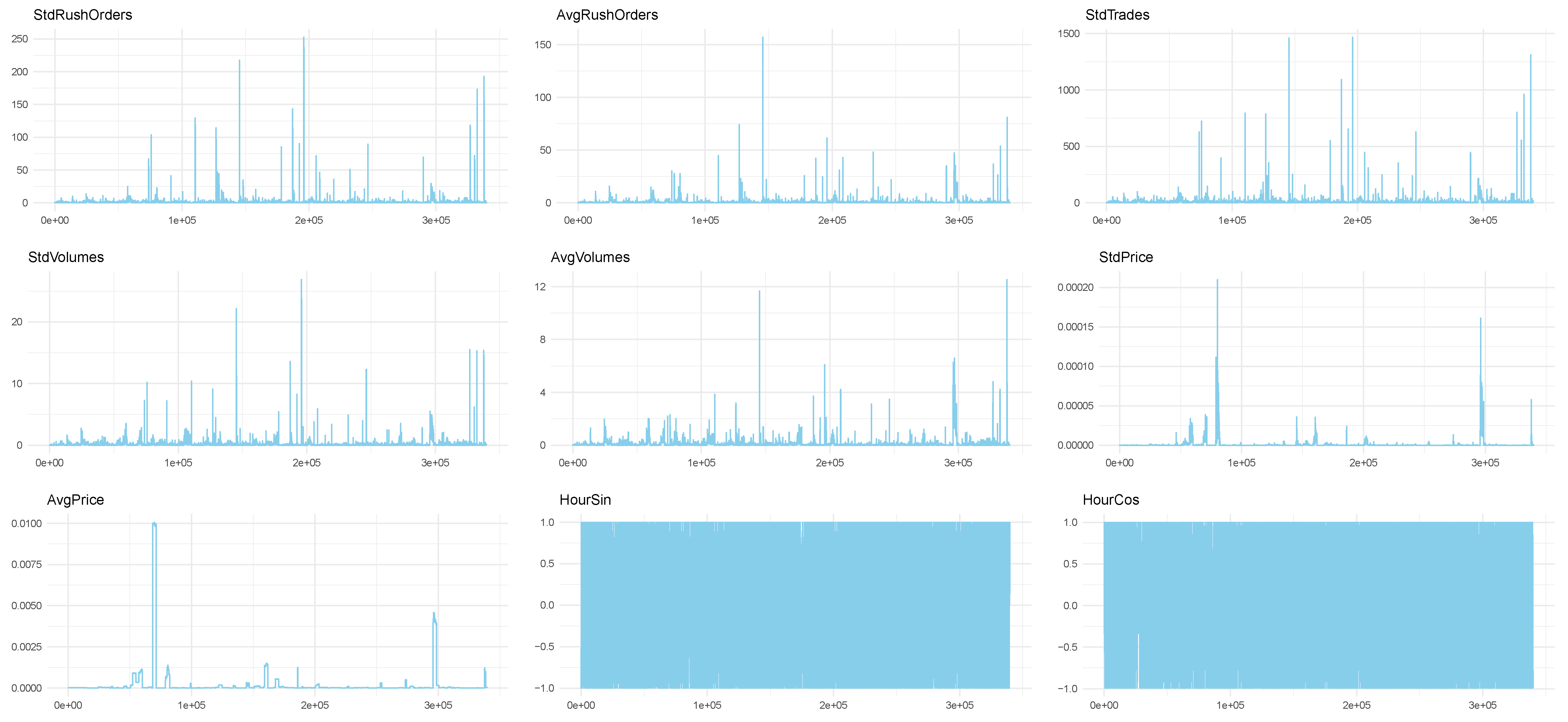
  • StdRushOrders and AvgRushOrders: the moving standard deviation and the average of the volume of rush orders in each chunk of the moving window.
  • StdTrades: the moving standard deviation of the number of trades.
  • StdVolumes and AvgVolumes: the moving standard deviation and the average of the volume of trades in each chunk of the moving window.
  • StdPrice and AvgPrice: the moving standard deviation and average of the closing price.
  • HourSin, HourCos, MinuteCos, MinuteSin: the hour and minute of the first transaction in each chunk. We used the sine and cosine functions to express their cyclical nature3.
We also tested the moving average of the maximum price in each chunk, as proposed in La Morgia et al. (2020, 2023). However, it was almost perfectly collinear with the average of the closing price and was not included in our analysis.
The number of data points corresponding to different combinations of chunk sizes and window sizes, and the frequency of detection of pump-and-dump schemes (i.e., the number of times where Y t = 1 ) in both levels and in %, when the pump-and-dump is flagged from the moment of the public announcement up to 60/120 s and 60 min before it, respectively, are reported in Table 4. The ADF and KPSS unit root test statistics for the average number of rush orders, average trade volumes, and average closing price, as well as the p-values of the Jarque–Bera normality tests, are presented in Table 5.
All the regressors used in our analysis, except MinuteCos and MinuteSin, which are too dense to be visible in a plot, for a chunk size of 60 s and a window size of 60 min are illustrated in Figure A1 in Appendix B. The plots for the other combinations of chunk sizes and window sizes are available from the authors upon request.
Table 4 indicates that the occurrence of Y t = 1 , signifying a pump-and-dump event, is very rare (less than 0.2% of all instances) if the pump-and-dump is flagged 1 or 2 min before the public announcement. The situation can be improved if we identify pump-and-dump schemes during the time between the public announcement and the 60-min period preceding it, which represents approximately 2.6% of all instances. As a result, detecting a pump-and-dump poses a considerable challenge. Moreover, while the regressors are generally stationary, their distribution strongly deviates from normality; see Table 5.4 In this regard, to evaluate the robustness of our analysis, we will also examine in Section 5 the potential utility of a generalized Box–Cox transformation that accounts for zero values, which may potentially improve the accuracy of classification.

4.2. Empirical Analysis

As previously discussed, we used various types of regressors in conjunction with three distinct classifiers (Logistic Regression, Random Forest, and the AdaBoost classifier) to identify the onset of a pump-and-dump scheme. Due to the limited number of pump-and-dump instances in our dataset, we did not partition the data into standard training and testing sets. Instead, we employed a 5-fold cross-validation method to obtain a more reliable performance evaluation (see also La Morgia et al. (2020, 2023) for similar approaches). For the random forest classifier, we employed a forest of 200 trees, with a maximum depth of 5 for each tree. For the AdaBoost classifier, we used 10 weak classifiers.
For the sake of space and interest, given the very large dataset at our disposal, we focused exclusively on the 5-fold cross-validation, whereas a small summary of the in-sample analysis can be found in the Appendix C.
Due to the large class imbalance in our dataset, we employed the resampling methods discussed in Section 3.1 to address this issue and we artificially balanced the dataset during model training. Resampling techniques used to create synthetic balanced datasets are also commonly referred to as “subsampling” techniques. The detailed implementation in R with the caret package can be found at https://topepo.github.io/caret/subsampling-for-class-imbalances.html, accessed on 1 December 2022. For our 5-fold cross-validation, we considered ten possible data configurations as follows:
1
Model training using the original dataset with pump-and-dumps flagged 1 or 2 min before the public announcement;
2–5
Model training using synthetic balanced data created with Random Under-Sampling (RUS), Random Over-Sampling (ROS), Synthetic Minority Over-sampling Technique (SMOTE), and the Random Over-Sampling Examples (ROSE) method, respectively, with pump-and-dumps flagged 1 or 2 min before the public announcement.
6
Model training using the original dataset with pump-and-dumps flagged 60 min before the public announcement;
7–10
Model training using synthetic balanced data created with Random Under-Sampling (RUS), Random Over-Sampling (ROS), Synthetic Minority Over-sampling Technique (SMOTE), and the Random Over-Sampling Examples (ROSE) method, respectively, with pump-and-dumps flagged 60 min before the public announcement.
The above-mentioned procedures were employed to train our three classifiers and evaluate their performances in detecting pump-and-dump schemes with crypto-assets. The following performance metrics were then used to evaluate the three competing classifiers:
  • Area under the Receiver Operating Characteristic (ROC) curve (AUC): it is a metric that measures the ability of a binary classification model to distinguish between positive and negative classes. It is calculated as the area under the receiver operating characteristic (ROC) curve, which plots the true positive rate against the false positive rate at various classification thresholds. AUC is commonly used to evaluate the overall performance of a classification model, and it ranges from 0 to 1, with a higher score indicating better performance; see Sammut and Webb (2011), pp. 869–75, and references therein for more details.
  • H-measure: the AUC has some well-known drawbacks, such as potentially providing misleading results when ROC curves cross. However, a more serious deficiency of the AUC (recognized only recently by Hand (2009) is that it is fundamentally incoherent in terms of misclassification costs, as it employs different misclassification cost distributions for different classifiers. This is problematic because the severity of misclassification for different points is a property of the problem rather than the classifiers that have been selected. The H-measure, proposed by Hand (2009) and Hand and Anagnostopoulos (2022), is a measure of classification performance that addresses the incoherence of AUC by introducing costs for different types of misclassification. However, it is common for the precise values of costs to be unknown at the time of classifier evaluation. To address this, they proposed taking the expectation over a distribution of likely cost values. While researchers should choose this distribution based on their knowledge of the problem, Hand (2009) and Hand and Anagnostopoulos (2022) also recommended a standard default distribution, such as beta distribution, for conventional measures, and they also generalized this approach to cover cases when class sizes are unknown. Moreover, in many problems, class sizes are extremely unbalanced (as in our case with pump-and-dumps), and it is rare to want to treat the two classes symmetrically. To address this issue, the H-measure requires a Severity Ratio (SR) that represents how much more severe misclassifying a class 0 instance is than misclassifying a class 1 instance. The severity ratio is formally defined as S R = c 0 / c 1 , where c 0 > 0 is the cost of misclassifying a class 0 datapoint as class 1. It is sometimes more convenient to consider the normalized cost c = c 0 / ( c 0 + c 1 ) , so that S R = c / ( 1 c ) , where c is in the range [0,1]. By default, the severity ratio is set to the reciprocal of the relative class frequency, i.e., S R = π ^ 1 / π ^ 0 , so that misclassifying the rare class is considered a graver mistake. For more detailed motivation of this default value, see Hand and Anagnostopoulos (2014).
  • Accuracy: it is a measure of the correct classification rate, which is the ratio of the number of correct predictions to the total number of predictions made. It is a widely used performance metric for binary classification, but it can be misleading in cases of imbalanced datasets.
  • Sensitivity: it measures the proportion of true positive predictions out of all the actual positive cases in the dataset. In other words, it measures how well the model identifies the positive cases correctly (in our case, the number of pump-and-dumps).
  • Specificity: it measures the proportion of true negative predictions out of all the actual negative cases in the dataset. In other words, it measures how well the model identifies the negative cases correctly.
The first two metrics are threshold-independent and do not depend on the specific choice of the threshold used to determine the final assigned class, whereas the last three metrics do depend on the choice of the threshold. In the latter case, we considered the following possible values:
  • p = 50 % : this is the classical level used in many applications in various fields;
  • p = 0.18 % : this level is close to the empirical frequency of pump-and-dumps in the dataset where they are flagged 1 or 2 min before the public announcement (that is, close to the so-called observed prevalence5, π ^ 1 , 1 o r 2 m i n . );
  • p = 2.6 % : this level is close to the empirical frequency of pump-and-dumps in the dataset where they are flagged 60 min before the public announcement ( π ^ 1 , 60 m i n . ).
We chose thresholds close to the observed prevalence because this is often the optimal choice for datasets with very low prevalence; see Freeman and Moisen (2008) and references therein for more details. We would like to emphasize that there are several methods available to select the optimal threshold, and the choice of the threshold ultimately depends on the cost function employed by the model user. Two large reviews with detailed applications in R software can be found in López-Ratón et al. (2014) and Thiele and Hirschfeld (2021).
The performance metrics of the 5-fold cross-validation for the ten possible data configurations, three classifiers, and for different chunk sizes and window sizes are reported in Table 6, Table 7, Table 8, Table 9, Table 10 and Table 11.
Table 6 reports the results for the original dataset with pump-and-dumps flagged 1 or 2 min before the public announcement, and it clearly demonstrates the impact of using classifiers with a heavily imbalanced dataset and a traditional threshold of p = 50 % on accuracy and sensitivity. The results show that accuracy is almost perfect, but sensitivity is close to zero, indicating an inability to detect a n y pump-and-dumps. However, by setting the threshold close to the observed prevalence ( p = 0.2 % ), the results significantly improved, with sensitivity exceeding 50% for both the random forest and logit models. AdaBoost, on the other hand, continued to struggle. If we use threshold-independent measures, the random forest model performs the best, while AdaBoost is the worst. Regarding chunk sizes and window sizes, the best results seem to be obtained with a chunk size of 30 s and a window size of 60 min, consistent with the findings reported in La Morgia et al. (2020, 2023).
When considering the original dataset with pump-and-dumps flagged 60 min before the public announcement (Table 9), the performance of both random forest and logit models improved significantly, with the random forest showing an AUC, H-measure, accuracy, sensitivity, and specificity remarkably close to 1 for almost all chunk sizes and window sizes. These metrics are the best across all 10 data configurations considered in this study. AdaBoost remained the worst model, although its metrics improved as well.
If we consider resampling methods to build synthetic balanced datasets with pump-and-dumps flagged 1 or 2 min before the announcement (Table 7 and Table 8), we can observe improvements in threshold-dependent metrics with p = 50 % , while there are no significant differences in threshold-dependent metrics with p = 0.18 % and threshold-independent metrics compared to the baseline case. However, particularly in the case of random forests together with Random Under-Sampling and ROSE methods, the results can be much worse. On the other hand, the AdaBoost classifier seems to benefit the most from resampling methods.
If we consider resampling methods to build synthetic balanced datasets with pump-and-dumps flagged 60 min before the announcement (Table 10 and Table 11), the results are generally better than the case with pump-and-dumps flagged 1 or 2 min before the announcement, with the exception of the ROSE method, which continues to show rather poor results. However, there are again no qualitative differences with the baseline case without resampling methods, which is worse only if threshold-dependent metrics with p = 50 % are considered.
The main result that emerges from this analysis is that the most effective approach to detecting pumps-and-dumps is by using the random forest model with a small chunk size (maximum of 30 s) and a window size of at least one hour, while setting the threshold close to the observed prevalence in the dataset for pump-and-dumps flagged 60 min before the announcement. Although resampling methods may be useful in some cases, particularly when using threshold-dependent metrics with p = 50 % , threshold-independent measures were not affected, and a better balance between sensitivity and specificity can be obtained by simply choosing a proper probability threshold. Moreover, detecting pump-and-dumps in real-time involves high-dimensional, high-frequency data, and the use of resampling methods to build synthetic datasets could be time-consuming, making such methods less practical. Additionally, implementing these methods for real-time detection would require a significant investment in hardware, which may not be feasible for crypto-exchanges and financial regulators due to the associated high financial costs.
Finally, we remark that our empirical analysis indirectly confirms the large-scale Monte Carlo simulations and case study in the medical field recently reported by van den Goorbergh et al. (2022), who showed that using Random Under-Sampling, Random Over-Sampling, and SMOTE methods resulted in poorly calibrated models that did not provide higher areas under the ROC curve compared to models developed without correction for class imbalance. Furthermore, they also showed that a better balance between sensitivity and specificity can be achieved by simply adjusting the probability threshold.

5. A Robustness Check: Transforming the Data Using a Generalized Box–Cox Tranformation

Even though all the regressors are stationary, some of them exhibit a large variability. Therefore, we investigated how our previous results would change by transforming the data to stabilize their variance. To achieve this, we transformed all the regressors (except for the four periodic functions of time) using the generalized version of the Box–Cox transformation proposed by Hawkins and Weisberg (2017). This method allows the inclusion of zeros and nonpositive values in the transformation. Their approach uses the original Box–Cox family of scaled power transformations, given by ( w λ 1 ) / λ for λ 0 and log ( w ) for λ = 0 , on the following transformed data:
w = 0.5 ( y + y 2 + γ 2 )
where y is the original data and λ and γ are either user-selected parameters or are estimated; see Hawkins and Weisberg (2017) for the full details on this transformation6.
The performance metric differences of the 5-fold cross-validation between the transformed datasets and the original datasets, with pump-and-dumps flagged 1 or 2 min before the public announcement, are reported in Table 12.
The differences are minimal and almost zero in all cases, indicating that using transformed regressors does not improve the classification process. This is a positive result, as computing the generalized Box–Cox transformation with high-dimensional and high-frequency data can be computationally demanding. The performance metric differences in the case of resampling methods used to build synthetic balanced data deliver qualitatively similar results. Therefore, for the sake of interest and space, they are not reported here.

6. Discussion and Conclusions

Detecting pump-and-dump schemes in the cryptocurrency market using high-frequency data is a daunting task due to the rarity of pump-and-dump cases in these datasets, which typically account for less than 0.2% of all cases. Additionally, despite VIP members of social media groups organizing these market manipulations, supposedly receiving detailed information about them seconds or minutes before the general public, unusual trading volumes can occur much earlier, which complicates the detection process. These challenges significantly affect the performance of any machine learning classifier employed to identify pump-and-dump activities, resulting in the difficulty of accurately detecting such instances in a timely manner.
To address the first problem, we proposed building synthetic balanced datasets generated according to four resampling methods for class imbalances proposed in the statistical literature. To address the second problem, we suggested flagging a pump-and-dump from the minute of the public announcement up to 60 min before it. This approach can deal with the insiders’ anticipated purchases of targeted crypto-assets and the issue of imbalanced datasets.
To verify the validity of our proposals, we collected data about pump-and-dump schemes from Pumpolymp, which is a website that provides detailed information about all Telegram groups dealing with crypto pump-and-dumps, and managed to extract 351 pump signals relative to the Binance crypto exchange that took place in 2021 and 2022. The historical transaction level data of the identified pumped coins were obtained using the CryptoCurrency eXchange Trading Library (CCXT). We used various types of regressors in conjunction with three distinct classifiers (logistic regression, random forest, and the AdaBoost classifier) to identify the onset of a pump-and-dump scheme.
Our empirical analysis showed that the most effective approach to detecting pump-and-dumps was using the original imbalanced dataset with pump-and-dumps flagged 60 min in advance, together with a random forest model with data segmented into 30-s chunks and regressors computed with a moving window of 1 h. We also found that a better balance between sensitivity and specificity could be achieved by merely adjusting the probability threshold, such as setting the threshold close to the observed prevalence in the original dataset. Although resampling methods were useful in some cases, particularly when using threshold-dependent metrics with a probability level equal to p = 50 % , threshold-independent measures were not affected, and in some cases they even provided worse AUC and H-measures compared to models developed without correction for class imbalance. Thus, our empirical evidence confirmed the large-scale Monte Carlo simulations performed by van den Goorbergh et al. (2022) who showed that using Random Under-Sampling, Random Over-Sampling, and SMOTE methods resulted in poorly calibrated models.
We highlight that detecting pump-and-dumps in real-time involves high-dimensional data, and the use of resampling methods to build synthetic datasets could be time-consuming, making such methods less practical. Implementing these methods for real-time detection would require a significant investment in hardware, which may not be feasible for crypto-exchanges and financial regulators due to the associated high financial costs.
Finally, we performed a set of robustness checks to verify that our results also held when transforming the data to stabilize their variance using a generalized version of the Box–Cox transformation to allow the inclusion of zeros and non-positive values. The differences were minimal, indicating that using transformed regressors did not improve the classification process.
We remark that we selected thresholds close to the observed prevalence because this is often the optimal choice for datasets with very low prevalence. However, the optimal threshold ultimately depends on the cost function employed by the model user. We leave a detailed analysis of the methods to find the optimal threshold to detect pump-and-dumps as an avenue for future research.
In the context of pump-and-dump scheme detection, it is important to acknowledge the potential for incorrect identifications and the impact this can have on the application of resampling methods to build synthetic balanced datasets. Our study assumes that all pump-and-dump schemes have been accurately identified through a separate empirical strategy. However, there is a possibility, if not likelihood, of noise or misclassifications in this higher-level identification process. The presence of incorrect identifications introduces a source of bias into the training sample used for model development. If the identification process exhibits a significant Type 1 error (false positive rate), the utilization of synthetic samples could potentially amplify this bias. This can be particularly problematic in cases of class imbalance, where the minority class (pump-and-dump schemes) may not be properly identified, resulting in an underrepresentation of the true positive cases. It is crucial to address this issue in future research. Conducting experiments on simulated data could provide valuable insights into the impact of misclassifications on the effectiveness of resampling methods. By intentionally introducing noise or biases in the identification process, researchers can examine how the use of synthetic samples exacerbates or mitigates these issues. Additionally, exploring alternative strategies for accurate identification of pump-and-dump schemes and assessing their influence on resampling techniques can contribute to the development of more robust and reliable models in the detection of this financial fraud. The robust methods and the large simulation studies in Bunkhumpornpat et al. (2009) and Barua et al. (2012) can provide valuable starting points.

Author Contributions

Conceptualization, D.F. and Y.X.; methodology, D.F. and Y.X.; software, D.F. and Y.X.; validation, D.F. and Y.X.; formal analysis, D.F.; investigation, D.F. and Y.X.; resources, D.F. and Y.X.; data curation, D.F. and Y.X.; writing—original draft preparation, D.F. and Y.X.; writing—review and editing, D.F.; visualization, D.F. and Y.X.; supervision, D.F.; project administration, D.F.; funding acquisition, D.F. All authors have read and agreed to the published version of the manuscript.

Funding

The first-named author gratefully acknowledges financial support from the grant of the Russian Science Foundation, n. 20-68-47030.

Data Availability Statement

The data are available from the authors upon request.

Conflicts of Interest

The authors declare no conflict of interest.

Appendix A

The RUS method reduces the number of instances in the majority class by randomly sampling from it until it matches the number of samples in the minority class. Suppose we have a dataset of n observations with a binary outcome variable Y that takes values 0 or 1, where Y = 1 denotes the event of interest. Let p be the proportion of observations with Y = 1 , so that p = n 1 / n , where n 1 is the number of observations with Y = 1 . Typically, p is much smaller than 0.5, indicating class imbalance. The RUS method involves randomly selecting a subset of observations with Y = 0 to match the number of observations with Y = 1 . Let n 0 be the number of observations with Y = 0 , so that n 0 = n n 1 . Then, we randomly select n 1 observations from the n 0 observations with Y = 0 to create a balanced dataset of 2 n 1 observations. RUS can be an effective method for addressing class imbalance, particularly when the dataset is large enough so that randomly selecting a subset of observations with Y = 0 does not result in loss of information. However, it may not work well if the dataset is small or if the minority class contains important information that is lost during under-sampling.
The ROS method involves randomly replicating observations with Y = 1 to create a balanced dataset. Specifically, we randomly select n 0 n 1 observations with replacement from the original n 1 observations with Y = 1 until we have a total of n 0 observations with Y = 1 . This results in a dataset where the number of observations with Y = 0 is equal to the number of observations with Y = 1 . ROS can be an effective method for addressing class imbalance, particularly when the dataset is small or when the minority class contains important information that should not be lost during under-sampling. However, it may not work well if the minority class contains outliers or noisy data.
SMOTE is a data augmentation method that creates synthetic minority class observations by interpolating between existing minority class observations. The basic idea is to identify each minority class observation and then create new synthetic observations by interpolating between it and its k nearest minority class neighbors. The SMOTE algorithm is performed through the following steps:
  • Identify the minority class observations with Y = 1 .
  • Randomly select a minority class observation x i from the dataset.
  • Find the k nearest minority class neighbors of x i in the feature space, where k is a user-defined parameter.
  • Create synthetic observations: for each nearest neighbor x j , generate a synthetic observation x i , n e w by randomly interpolating between x i and x j in the feature space:
    x i , n e w = x i + r a n d ( 0 , 1 ) · ( x j x i )
    where r a n d ( 0 , 1 ) is a random number between 0 and 1.
  • Repeat steps 2–4 until the desired number of synthetic observations have been generated.
SMOTE can be an effective method for addressing class imbalance, particularly when the dataset is small and when the minority class is not close to the majority class in the feature space. However, it may not work well if the minority class is sparse or if there is high overlap between the minority and majority classes in the feature space. Additionally, the choice of k can impact the effectiveness of the algorithm, as larger values of k can result in more diverse synthetic observations, but can also increase the risk of introducing noise or outliers.
The ROSE technique aims to address class imbalance by generating artificial samples from the feature space neighbourhood around the minority class. This technique combines over-sampling and under-sampling, and comprises four steps:
  • Resample the majority class data using a bootstrap resampling technique to reduce the number of majority class samples to a ratio of 50% via under-sampling.
  • Resample the minority class data using a bootstrap resampling technique to increase the number of minority class samples to a ratio of 50% via over-sampling.
  • Combined the data from steps 1 and 2 to create a new training sample.
  • Generate new synthetic data for both the majority and minority classes in their respective neighborhoods. The neighborhood shape is defined by the kernel density function with a Gaussian kernel K H j and a smoothing matrix H j , j = 0 , 1 , with a d dimension (where d is the number of independent variables), where H j = d i a g ( h 1 ( j ) , , h d ( j ) ) and h d ( j ) is defined as follows:
    h q ( j ) = 4 ( d + 2 ) n 1 / ( d + 4 ) · σ ^ q ( j ) , q = 1 , , d .
    Here, σ ^ q ( j ) is the standard deviation of the q-th dimension of the observations belonging to a given class.
These four steps are repeated for each training sample to produce a new synthetic training sample of approximately equal size as the original dataset, with the number of instances for both classes being equally represented. The ROSE technique represents an effective method for generating synthetic samples, as it leverages the available information to synthesize new samples that are more representative of the minority class. Moreover, using the synthetic generation of new examples in ROSE strengthens the learning process and estimates the distribution of the chosen measure of accuracy. The artificial training set can be used to estimate the classification model, while the originally observed data are reserved for testing the classifier. Alternatively, cross-validation or smoothed bootstrap methods can be used. Creating new artificial examples from an estimate of the conditional densities of the two classes allows for overcoming the limits of both the apparent error and the holdout method, which are not advisable in extreme imbalanced learning due to the scarcity of rare class data.

Appendix B

Figure A1. Regressors used in the empirical analysis (except for MinuteCos and MinuteSin) for a chunk size of 60 s and a window size of 60 min.
Econometrics 11 00022 g0a1

Appendix C

For the sake of space and interest, we provide a condensed summary of the in-sample empirical results using the complete data sample for a chunk size of 60 s and a window size of 60 min7. The full set of results are available from the authors upon request. The parameter estimates for the logit model can be found in Table A1, while Figure A2 displays the variable importance plots as measured by the random forest model (see Breiman (2001) and Strobl et al. (2007) for the mathematical details of these importance measures).
We remark that the logit regression may encounter significant challenges in the presence of class imbalance; see King and Zeng (2001), He and Garcia (2009), and Sun et al. (2009). Similarly, the variable importance measures computed using random forests may be misspecified in the case of extreme class imbalance, as in our study; see Janitza et al. (2013) for a detailed discussion. Therefore, we advise interpreting the reported results cautiously. This is precisely why our main analysis focuses on forecasting for real-time detection of pump-and-dump schemes, rather than on identifying the most influential variables.
Table A1. Parameters estimates of the logit model with the full data sample.
EstimateStd. Errorz ValuePr (>|z|)
(Intercept)−4.01030.0162−247.020.0000
std_order0.14460.01549.360.0000
avg_order−0.24730.0248−9.970.0000
std_trades−0.01440.0023−6.310.0000
std_volume−0.16150.0849−1.900.0572
avg_volume0.69750.15054.630.0000
std_price40,943.05512073.120119.750.0000
avg_price−66.399414.6226−4.540.0000
hour_sin−0.66540.0181−36.840.0000
hour_cos−1.11780.0196−56.960.0000
minute_sin−0.03800.0156−2.430.0150
minute_cos0.03320.01522.180.0291
Figure A2. Variable importance measures for the random forest model.
Econometrics 11 00022 g0a2

Appendix D

Figure A3. Buy (+) and sell (−) orders 24 h prior to the announced pump-and-dump. The x-axis represents 1-h intervals. Buy/sell orders that were three standard deviations above/below the mean were identified as outliers and highlighted in red. P&Ds from n. 1 to n. 8.
Econometrics 11 00022 g0a3
Figure A4. Buy (+) and sell (−) orders 24 h prior to the announced pump-and-dump. The x-axis represents 1-h intervals. Buy/sell orders that were three standard deviations above/below the mean were identified as outliers and highlighted in red. P&Ds from n. 9 to n. 16.
Econometrics 11 00022 g0a4
Figure A5. Buy (+) and sell (−) orders 24 h prior to the announced pump-and-dump. The x-axis represents 1-h intervals. Buy/sell orders that were three standard deviations above/below the mean were identified as outliers and highlighted in red. P&Ds from n. 17 to n. 24.
Econometrics 11 00022 g0a5
Figure A6. Buy (+) and sell (−) orders 24 h prior to the announced pump-and-dump. The x-axis represents 1-h intervals. Buy/sell orders that were three standard deviations above/below the mean were identified as outliers and highlighted in red. P&Ds from n. 25 to n. 32.
Econometrics 11 00022 g0a6
Figure A7. Buy (+) and sell (−) orders 24 h prior to the announced pump-and-dump. The x-axis represents 1-h intervals. Buy/sell orders that were three standard deviations above/below the mean were identified as outliers and highlighted in red. P&Ds from n. 33 to n. 40.
Econometrics 11 00022 g0a7
Figure A8. Buy (+) and sell (−) orders 24 h prior to the announced pump-and-dump. The x-axis represents 1-h intervals. Buy/sell orders that were three standard deviations above/below the mean were identified as outliers and highlighted in red. P&Ds from n. 41 to n. 48.
Econometrics 11 00022 g0a8
Figure A9. Buy (+) and sell (−) orders 24 h prior to the announced pump-and-dump. The x-axis represents 1-h intervals. Buy/sell orders that were three standard deviations above/below the mean were identified as outliers and highlighted in red. P&Ds from n. 49 to n. 56.
Econometrics 11 00022 g0a9
Figure A10. Buy (+) and sell (−) orders 24 h prior to the announced pump-and-dump. The x-axis represents 1-h intervals. Buy/sell orders that were three standard deviations above/below the mean were identified as outliers and highlighted in red. P&Ds from n. 57 to n. 64.
Econometrics 11 00022 g0a10
Figure A11. Buy (+) and sell (−) orders 24 h prior to the announced pump-and-dump. The x-axis represents 1-h intervals. Buy/sell orders that were three standard deviations above/below the mean were identified as outliers and highlighted in red. P&Ds from n. 65 to n. 72.
Econometrics 11 00022 g0a11
Figure A12. Buy (+) and sell (−) orders 24 h prior to the announced pump-and-dump. The x-axis represents 1-h intervals. Buy/sell orders that were three standard deviations above/below the mean were identified as outliers and highlighted in red. P&Ds from n. 73 to n. 80.
Econometrics 11 00022 g0a12
Figure A13. Buy (+) and sell (−) orders 24 h prior to the announced pump-and-dump. The x-axis represents 1-h intervals. Buy/sell orders that were three standard deviations above/below the mean were identified as outliers and highlighted in red. P&Ds from n. 81 to n. 88.
Econometrics 11 00022 g0a13
Figure A14. Buy (+) and sell (−) orders 24 h prior to the announced pump-and-dump. The x-axis represents 1-h intervals. Buy/sell orders that were three standard deviations above/below the mean were identified as outliers and highlighted in red. P&Ds from n. 89 to n. 96.
Econometrics 11 00022 g0a14
Figure A15. Buy (+) and sell (−) orders 24 h prior to the announced pump-and-dump. The x-axis represents 1-h intervals. Buy/sell orders that were three standard deviations above/below the mean were identified as outliers and highlighted in red. P&Ds from n. 97 to n. 104.
Econometrics 11 00022 g0a15
Figure A16. Buy (+) and sell (−) orders 24 h prior to the announced pump-and-dump. The x-axis represents 1-h intervals. Buy/sell orders that were three standard deviations above/below the mean were identified as outliers and highlighted in red. P&Ds from n. 105 to n. 112.
Econometrics 11 00022 g0a16
Figure A17. Buy (+) and sell (−) orders 24 h prior to the announced pump-and-dump. The x-axis represents 1-h intervals. Buy/sell orders that were three standard deviations above/below the mean were identified as outliers and highlighted in red. P&Ds from n. 113 to n. 120.
Econometrics 11 00022 g0a17
Figure A18. Buy (+) and sell (−) orders 24 h prior to the announced pump-and-dump. The x-axis represents 1-h intervals. Buy/sell orders that were three standard deviations above/below the mean were identified as outliers and highlighted in red. P&Ds from n. 121 to n. 128.
Econometrics 11 00022 g0a18
Figure A19. Buy (+) and sell (−) orders 24 h prior to the announced pump-and-dump. The x-axis represents 1-h intervals. Buy/sell orders that were three standard deviations above/below the mean were identified as outliers and highlighted in red. P&Ds from n. 129 to n. 136.
Econometrics 11 00022 g0a19
Figure A20. Buy (+) and sell (−) orders 24 h prior to the announced pump-and-dump. The x-axis represents 1-h intervals. Buy/sell orders that were three standard deviations above/below the mean were identified as outliers and highlighted in red. P&Ds from n. 137 to n. 144.
Econometrics 11 00022 g0a20
Figure A21. Buy (+) and sell (−) orders 24 h prior to the announced pump-and-dump. The x-axis represents 1-h intervals. Buy/sell orders that were three standard deviations above/below the mean were identified as outliers and highlighted in red. P&Ds from n. 145 to n. 152.
Econometrics 11 00022 g0a21
Figure A22. Buy (+) and sell (−) orders 24 h prior to the announced pump-and-dump. The x-axis represents 1-h intervals. Buy/sell orders that were three standard deviations above/below the mean were identified as outliers and highlighted in red. P&Ds from n. 153 to n. 160.
Econometrics 11 00022 g0a22
Figure A23. Buy (+) and sell (−) orders 24 h prior to the announced pump-and-dump. The x-axis represents 1-h intervals. Buy/sell orders that were three standard deviations above/below the mean were identified as outliers and highlighted in red. P&Ds from n. 161 to n. 168.
Econometrics 11 00022 g0a23
Figure A24. Buy (+) and sell (−) orders 24 h prior to the announced pump-and-dump. The x-axis represents 1-h intervals. Buy/sell orders that were three standard deviations above/below the mean were identified as outliers and highlighted in red. P&Ds from n. 169 to n. 176.
Econometrics 11 00022 g0a24
Figure A25. Buy (+) and sell (−) orders 24 h prior to the announced pump-and-dump. The x-axis represents 1-h intervals. Buy/sell orders that were three standard deviations above/below the mean were identified as outliers and highlighted in red. P&Ds from n. 177 to n. 184.
Econometrics 11 00022 g0a25
Figure A26. Buy (+) and sell (−) orders 24 h prior to the announced pump-and-dump. The x-axis represents 1-h intervals. Buy/sell orders that were three standard deviations above/below the mean were identified as outliers and highlighted in red. P&Ds from n. 185 to n. 192.
Econometrics 11 00022 g0a26
Figure A27. Buy (+) and sell (−) orders 24 h prior to the announced pump-and-dump. The x-axis represents 1-h intervals. Buy/sell orders that were three standard deviations above/below the mean were identified as outliers and highlighted in red. P&Ds from n. 193 to n. 200.
Econometrics 11 00022 g0a27
Figure A28. Buy (+) and sell (−) orders 24 h prior to the announced pump-and-dump. The x-axis represents 1-h intervals. Buy/sell orders that were three standard deviations above/below the mean were identified as outliers and highlighted in red. P&Ds from n. 201 to n. 208.
Econometrics 11 00022 g0a28
Figure A29. Buy (+) and sell (−) orders 24 h prior to the announced pump-and-dump. The x-axis represents 1-h intervals. Buy/sell orders that were three standard deviations above/below the mean were identified as outliers and highlighted in red. P&Ds from n. 209 to n. 216.
Econometrics 11 00022 g0a29
Figure A30. Buy (+) and sell (−) orders 24 h prior to the announced pump-and-dump. The x-axis represents 1-h intervals. Buy/sell orders that were three standard deviations above/below the mean were identified as outliers and highlighted in red. P&Ds from n. 217 to n. 224.
Econometrics 11 00022 g0a30
Figure A31. Buy (+) and sell (−) orders 24 h prior to the announced pump-and-dump. The x-axis represents 1-h intervals. Buy/sell orders that were three standard deviations above/below the mean were identified as outliers and highlighted in red. P&Ds from n. 225 to n. 232.
Econometrics 11 00022 g0a31
Figure A32. Buy (+) and sell (−) orders 24 h prior to the announced pump-and-dump. The x-axis represents 1-h intervals. Buy/sell orders that were three standard deviations above/below the mean were identified as outliers and highlighted in red. P&Ds from n. 233 to n. 240.
Econometrics 11 00022 g0a32
Figure A33. Buy (+) and sell (−) orders 24 h prior to the announced pump-and-dump. The x-axis represents 1-h intervals. Buy/sell orders that were three standard deviations above/below the mean were identified as outliers and highlighted in red. P&Ds from n. 241 to n. 248.
Econometrics 11 00022 g0a33
Figure A34. Buy (+) and sell (−) orders 24 h prior to the announced pump-and-dump. The x-axis represents 1-h intervals. Buy/sell orders that were three standard deviations above/below the mean were identified as outliers and highlighted in red. P&Ds from n. 249 to n. 256.
Econometrics 11 00022 g0a34
Figure A35. Buy (+) and sell (−) orders 24 h prior to the announced pump-and-dump. The x-axis represents 1-h intervals. Buy/sell orders that were three standard deviations above/below the mean were identified as outliers and highlighted in red. P&Ds from n. 257 to n. 264.
Econometrics 11 00022 g0a35
Figure A36. Buy (+) and sell (−) orders 24 h prior to the announced pump-and-dump. The x-axis represents 1-h intervals. Buy/sell orders that were three standard deviations above/below the mean were identified as outliers and highlighted in red. P&Ds from n. 265 to n. 272.
Econometrics 11 00022 g0a36
Figure A37. Buy (+) and sell (−) orders 24 h prior to the announced pump-and-dump. The x-axis represents 1-h intervals. Buy/sell orders that were three standard deviations above/below the mean were identified as outliers and highlighted in red. P&Ds from n. 273 to n. 280.
Econometrics 11 00022 g0a37
Figure A38. Buy (+) and sell (−) orders 24 h prior to the announced pump-and-dump. The x-axis represents 1-h intervals. Buy/sell orders that were three standard deviations above/below the mean were identified as outliers and highlighted in red. P&Ds from n. 281 to n. 288.
Econometrics 11 00022 g0a38
Figure A39. Buy (+) and sell (−) orders 24 h prior to the announced pump-and-dump. The x-axis represents 1-h intervals. Buy/sell orders that were three standard deviations above/below the mean were identified as outliers and highlighted in red. P&Ds from n. 289 to n. 296.
Econometrics 11 00022 g0a39
Figure A40. Buy (+) and sell (−) orders 24 h prior to the announced pump-and-dump. The x-axis represents 1-h intervals. Buy/sell orders that were three standard deviations above/below the mean were identified as outliers and highlighted in red. P&Ds from n. 297 to n. 304.
Econometrics 11 00022 g0a40
Figure A41. Buy (+) and sell (−) orders 24 h prior to the announced pump-and-dump. The x-axis represents 1-h intervals. Buy/sell orders that were three standard deviations above/below the mean were identified as outliers and highlighted in red. P&Ds from n. 305 to n. 312.
Econometrics 11 00022 g0a41
Figure A42. Buy (+) and sell (−) orders 24 h prior to the announced pump-and-dump. The x-axis represents 1-h intervals. Buy/sell orders that were three standard deviations above/below the mean were identified as outliers and highlighted in red. P&Ds from n. 313 to n. 320.
Econometrics 11 00022 g0a42
Figure A43. Buy (+) and sell (−) orders 24 h prior to the announced pump-and-dump. The x-axis represents 1-h intervals. Buy/sell orders that were three standard deviations above/below the mean were identified as outliers and highlighted in red. P&Ds from n. 321 to n. 328.
Econometrics 11 00022 g0a43
Figure A44. Buy (+) and sell (−) orders 24 h prior to the announced pump-and-dump. The x-axis represents 1-h intervals. Buy/sell orders that were three standard deviations above/below the mean were identified as outliers and highlighted in red. P&Ds from n. 329 to n. 336.
Econometrics 11 00022 g0a44
Figure A45. Buy (+) and sell (−) orders 24 h prior to the announced pump-and-dump. The x-axis represents 1-h intervals. Buy/sell orders that were three standard deviations above/below the mean were identified as outliers and highlighted in red. P&Ds from n. 337 to n. 344.
Econometrics 11 00022 g0a45
Figure A46. Buy (+) and sell (−) orders 24 h prior to the announced pump-and-dump. The x-axis represents 1-h intervals. Buy/sell orders that were three standard deviations above/below the mean were identified as outliers and highlighted in red. P&Ds from n. 345 to n. 351.
Econometrics 11 00022 g0a46

Notes

1
https://pumpolymp.com (accessed on 1 December 2022).
2
https://github.com/ccxt/ccxt (accessed on 1 December 2022).
3
The four periodic regressors were computed as originally proposed by La Morgia et al. (2020, 2023):
H o u r S i n : sin ( 2 · π · h o u r / 23 ) H o u r C o s : cos ( 2 · π · h o u r / 23 ) M i n u t e S i n : sin ( 2 · π · m i n u t e / 59 ) M i n u t e C o s : cos ( 2 · π · m i n u t e / 59 )
The original Python code used by La Morgia et al. (2020, 2023) to compute these regressors can be found at https://github.com/SystemsLab-Sapienza/pump-and-dump-dataset/blob/master/features.py (accessed on 1 December 2022).
4
For a couple of combinations of chunk sizes and window sizes, both ADF and KPSS tests rejected their null hypotheses. We remark that a lack a unit root does not immediately imply (strict) stationarity. Moreover, strong heteroskedasticity, nonlinear time trends, or other reasons can make a time series non stationary. Furthermore, there is simulation evidence showing that the ADF test should be preferred in the case of a large time sample; see Arltová and Fedorová (2016) and references therein. It is for all these reasons that we will also use a generalized Box–Cox transformation to evaluate the robustness of our analysis.
5
The observed prevalence is the proportion of positive cases in the actual dataset, which is calculated as the number of positive cases divided by the total number of cases in the dataset.
6
This generalization of the Box–Cox transformation is implemented in the R package car.
7
The authors want to thank an anonymous referee for bringing this issue to our attention.

References

  1. Akbani, Rehan, Stephen Kwek, and Nathalie Japkowicz. 2004. Applying support vector machines to imbalanced datasets. In Machine Learning: ECML 2004: 15th European Conference on Machine Learning, Pisa, Italy, September 20–24. 2004. Proceedings 15. Berlin: Springer, pp. 39–50. [Google Scholar]
  2. Antonopoulos, Andreas. 2014. Mastering Bitcoin: Unlocking Digital Cryptocurrencies. Sonoma County: O’Reilly Media, Inc. [Google Scholar]
  3. Arltová, Markéta, and Darina Fedorová. 2016. Selection of Unit Root Test on the Basis of Length of the Time Series and Value of AR(1) Parameter. Statistika: Statistics & Economy Journal 96: 47–64. [Google Scholar]
  4. Barua, Sukarna, Md Monirul Islam, Xin Yao, and Kazuyuki Murase. 2012. MWMOTE–majority weighted minority oversampling technique for imbalanced data set learning. IEEE Transactions on Knowledge and Data Engineering 26: 405–25. [Google Scholar] [CrossRef]
  5. Bouraoui, Taoufik. 2015. Does’ pump and dump’affect stock markets? International Journal of Trade, Economics and Finance 6: 45. [Google Scholar] [CrossRef]
  6. Breiman, Leo. 2001. Random forests. Machine Learning 45: 5–32. [Google Scholar] [CrossRef]
  7. Breiman, Leo, Jerome Friedman, Richard Olshen, and Charles Stone. 1984. Classification and Regression Trees. Monterey: Wadsworth & Brooks. [Google Scholar]
  8. Bunkhumpornpat, Chumphol, Krung Sinapiromsaran, and Chidchanok Lursinsap. 2009. Safe-level-smote: Safe-level-synthetic minority over-sampling technique for handling the class imbalanced problem. In Advances in Knowledge Discovery and Data Mining: 13th Pacific-Asia Conference, PAKDD 2009 Bangkok, Thailand, April 27–30. Proceedings 13. Berlin: Springer, pp. 475–82. [Google Scholar]
  9. Charu, C. Aggarwal. 2019. Outlier Analysis. Berlin: Springer. [Google Scholar]
  10. Chawla, Nitesh V. 2003. C4. 5 and imbalanced data sets: Investigating the effect of sampling method, probabilistic estimate, and decision tree structure. In Proceedings of the ICML. Toronto: CIBC, vol. 3, p. 66. [Google Scholar]
  11. Chawla, Nitesh V., Kevin W. Bowyer, Lawrence O. Hall, and W. Philip Kegelmeyer. 2002. Smote: Synthetic minority over-sampling technique. Journal of Artificial Intelligence Research 16: 321–57. [Google Scholar] [CrossRef]
  12. Cieslak, David A., and Nitesh V. Chawla. 2008. Learning decision trees for unbalanced data. In Machine Learning and Knowledge Discovery in Databases: European Conference, ECML PKDD 2008, Antwerp, Belgium, September 15–19. Proceedings, Part I 19. Berlin: Springer, pp. 241–56. [Google Scholar]
  13. Dhawan, Anirudh, and Tālis Putniņš. 2023. A new wolf in town? pump-and-dump manipulation in cryptocurrency markets. Review of Finance 27: 935–75. [Google Scholar] [CrossRef]
  14. Feder, Amir, Neil Gandal, J. T. Hamrick, Tyler Moore, Arghya Mukherjee, Farhang Rouhi, and Marie Vasek. 2018. The Economics of Cryptocurrency Pump and Dump Schemes. Technical Report, CEPR Discussion Papers, No. 13404. London: Centre for Economic Policy Research. [Google Scholar]
  15. Freeman, Elizabeth A., and Gretchen G. Moisen. 2008. A comparison of the performance of threshold criteria for binary classification in terms of predicted prevalence and kappa. Ecological Modelling 217: 48–58. [Google Scholar] [CrossRef]
  16. Frieder, Laura, and Jonathan Zittrain. 2008. Spam works: Evidence from stock touts and corresponding market activity. Hastings Communications and Entertainment Law Journal 30: 479–520. [Google Scholar] [CrossRef]
  17. Guo, Hongyu, and Herna L. Viktor. 2004. Boosting with data generation: Improving the classification of hard to learn examples. In Innovations in Applied Artificial Intelligence: 17th International Conference on Industrial and Engineering Applications of Artificial Intelligence and Expert Systems, IEA/AIE 2004, Ottawa, Canada, May 17–20. Proceedings 17. Berlin: Springer, pp. 1082–91. [Google Scholar]
  18. Hamrick, J. T., Farhang Rouhi, Arghya Mukherjee, Amir Feder, Neil Gandal, Tyler Moore, and Marie Vasek. 2021. An examination of the cryptocurrency pump-and-dump ecosystem. Information Processing & Management 58: 102506. [Google Scholar]
  19. Hand, David J. 2009. Measuring classifier performance: A coherent alternative to the area under the roc curve. Machine Learning 77: 103–23. [Google Scholar] [CrossRef]
  20. Hand, David J., and Christoforos Anagnostopoulos. 2014. A better beta for the h measure of classification performance. Pattern Recognition Letters 40: 41–46. [Google Scholar] [CrossRef]
  21. Hand, David J., and Christoforos Anagnostopoulos. 2022. Notes on the h-measure of classifier performance. Advances in Data Analysis and Classification 17: 109–24. [Google Scholar] [CrossRef]
  22. Hand, David J., and Veronica Vinciotti. 2003. Choosing k for two-class nearest neighbour classifiers with unbalanced classes. Pattern Recognition Letters 24: 1555–62. [Google Scholar] [CrossRef]
  23. Hastie, Trevor, Robert Tibshirani, and Jerome Friedman. 2017. The Elements of Statistical Learning: Data Mining, Inference, and Prediction, 2nd ed. 12th Printing. Berlin: Springer. [Google Scholar]
  24. Hawkins, D. M., and S. Weisberg. 2017. Combining the box-cox power and generalised log transformations to accommodate nonpositive responses in linear and mixed-effects linear models. South African Statistical Journal 51: 317–28. [Google Scholar] [CrossRef]
  25. He, Haibo, and Edwardo A. Garcia. 2009. Learning from imbalanced data. IEEE Transactions on Knowledge and Data Engineering 21: 1263–84. [Google Scholar]
  26. Janitza, Silke, Carolin Strobl, and Anne-Laure Boulesteix. 2013. An auc-based permutation variable importance measure for random forests. BMC Bioinformatics 14: 119. [Google Scholar] [CrossRef]
  27. Kamps, Josh, and Bennett Kleinberg. 2018. To the moon: Defining and detecting cryptocurrency pump-and-dumps. Crime Science 7: 18. [Google Scholar] [CrossRef]
  28. King, Gary, and Langche Zeng. 2001. Logistic regression in rare events data. Political Analysis 9: 137–63. [Google Scholar] [CrossRef]
  29. Kotsiantis, Sotiris, Dimitris Kanellopoulos, and Panayiotis Pintelas. 2006. Handling imbalanced datasets: A review. GESTS International Transactions on Computer Science and Engineering 30: 25–36. [Google Scholar]
  30. Krinklebine, Karlos. 2010. Hacking Wall Street: Attacks And Countermeasures. Chicago: Independently Published. [Google Scholar]
  31. Kukar, Matjaz, and Igor Kononenko. 1998. Cost sensitive learning with neural networks. In ECAI 98: 13th European Conference on Artificial Intelligence. Hoboken: John Wiley & Sons, Ltd., vol. 15, pp. 88–94. [Google Scholar]
  32. La Morgia, Massimo, Alessandro Mei, Francesco Sassi, and Julinda Stefa. 2020. Pump and dumps in the bitcoin era: Real time detection of cryptocurrency market manipulations. Paper presented at 2020 29th International Conference on Computer Communications and Networks (ICCCN), Honolulu, HI, USA, August 3–6; pp. 1–9. [Google Scholar]
  33. La Morgia, Massimo, Alessandro Mei, Francesco Sassi, and Julinda Stefa. 2023. The doge of wall street: Analysis and detection of pump and dump cryptocurrency manipulations. ACM Transactions on Internet Technology 23: 1–28. [Google Scholar] [CrossRef]
  34. Lee, Sauchi Stephen. 1999. Regularization in skewed binary classification. Computational Statistics 14: 277–92. [Google Scholar] [CrossRef]
  35. Lin, Yi, Yoonkyung Lee, and Grace Wahba. 2002. Support vector machines for classification in nonstandard situations. Machine Learning 46: 191–202. [Google Scholar] [CrossRef]
  36. López-Ratón, Mónica, María Xosé Rodríguez-Álvarez, Carmen Cadarso-Suárez, and Francisco Gude-Sampedro. 2014. OptimalCutpoints: An R package for selecting optimal cutpoints in diagnostic tests. Journal of Statistical Software 61: 1–36. [Google Scholar] [CrossRef]
  37. Lunardon, Nicola, Giovanna Menardi, and Nicola Torelli. 2014. Rose: A package for binary imbalanced learning. R Journal 6: 79–89. [Google Scholar] [CrossRef]
  38. McCarthy, Kate, Bibi Zabar, and Gary Weiss. 2005. Does cost-sensitive learning beat sampling for classifying rare classes? In Proceedings of the 1st International Workshop on Utility-Based Data Mining. New York: Gary Weiss, pp. 69–77. [Google Scholar]
  39. Mease, David, Abraham J. Wyner, and Andreas Buja. 2007. Boosted classification trees and class probability/quantile estimation. Journal of Machine Learning Research 8: 409–39. [Google Scholar]
  40. Menardi, Giovanna, and Nicola Torelli. 2014. Training and assessing classification rules with imbalanced data. Data Mining and Knowledge Discovery 28: 92–122. [Google Scholar] [CrossRef]
  41. Narayanan, Arvind, Joseph Bonneau, Edward Felten, Andrew Miller, and Steven Goldfeder. 2016. Bitcoin and Cryptocurrency Technologies: A Comprehensive Introduction. Princeton: Princeton University Press. [Google Scholar]
  42. Nghiem, Huy, Goran Muric, Fred Morstatter, and Emilio Ferrara. 2021. Detecting cryptocurrency pump-and-dump frauds using market and social signals. Expert Systems with Applications 182: 115284. [Google Scholar] [CrossRef]
  43. Ouyang, Liangyi, and Bolong Cao. 2020. Selective pump-and-dump: The manipulation of their top holdings by chinese mutual funds around quarter-ends. Emerging Markets Review 44: 100697. [Google Scholar] [CrossRef]
  44. Pukelsheim, Friedrich. 1994. The three sigma rule. The American Statistician 48: 88–91. [Google Scholar]
  45. Riddle, Patricia, Richard Segal, and Oren Etzioni. 1994. Representation design and brute-force induction in a boeing manufacturing domain. Applied Artificial Intelligence an International Journal 8: 125–47. [Google Scholar] [CrossRef]
  46. Rousseeuw, Peter J., and Annick M. Leroy. 2005. Robust Regression and Outlier Detection. Hoboken: John Wiley & Sons. [Google Scholar]
  47. Sammut, Claude, and Geoffrey Webb. 2011. Encyclopedia of Machine Learning. Berlin: Springer. [Google Scholar]
  48. Schiavo, Rosa A., and David J. Hand. 2000. Ten more years of error rate research. International Statistical Review 68: 295–310. [Google Scholar] [CrossRef]
  49. Shao, Sisi. 2021. The effectiveness of supervised learning models in detection of pump and dump activity in dogecoin. In Second IYSF Academic Symposium on Artificial Intelligence and Computer Engineering. Bellingham: SPIE, Volume 12079, pp. 356–63. [Google Scholar]
  50. Siering, Michael. 2019. The economics of stock touting during internet-based pump and dump campaigns. Information Systems Journal 29: 456–83. [Google Scholar] [CrossRef]
  51. Siris, Vasilios A., and Fotini Papagalou. 2004. Application of anomaly detection algorithms for detecting syn flooding attacks. Paper presented at IEEE Global Telecommunications Conference, GLOBECOM’04, Dallas, TX, USA, November 29–December 3; Volume 4, pp. 2050–54. [Google Scholar]
  52. Strobl, Carolin, Anne-Laure Boulesteix, Achim Zeileis, and Torsten Hothorn. 2007. Bias in random forest variable importance measures: Illustrations, sources and a solution. BMC Bioinformatics 8: 25. [Google Scholar] [CrossRef] [PubMed]
  53. Sun, Yanmin, Andrew K. C. Wong, and Mohamed S. Kamel. 2009. Classification of imbalanced data: A review. International Journal of Pattern Recognition and Artificial Intelligence 23: 687–719. [Google Scholar] [CrossRef]
  54. Tantithamthavorn, Chakkrit, Ahmed E. Hassan, and Kenichi Matsumoto. 2018. The impact of class rebalancing techniques on the performance and interpretation of defect prediction models. IEEE Transactions on Software Engineering 46: 1200–19. [Google Scholar] [CrossRef]
  55. Thiele, Christian, and Gerrit Hirschfeld. 2021. Cutpointr: Improved Estimation and Validation of Optimal Cutpoints in R. Journal of Statistical Software 98: 1–27. [Google Scholar] [CrossRef]
  56. Ting, Kai Ming. 2002. An instance-weighting method to induce cost-sensitive trees. IEEE Transactions on Knowledge and Data Engineering 14: 659–65. [Google Scholar] [CrossRef]
  57. US Security and Exchange Commission. 2005. Pump&Dump.con: Tips for Avoiding Stock Scams on the Internet; Technical Report. Washington, DC: US Security and Exchange Commission.
  58. van den Goorbergh, Ruben, Maarten van Smeden, Dirk Timmerman, and Ben Van Calster. 2022. The harm of class imbalance corrections for risk prediction models: Illustration and simulation using logistic regression. Journal of the American Medical Informatics Association 29: 1525–34. [Google Scholar] [CrossRef]
  59. Victor, Friedhelm, and Tanja Hagemann. 2019. Cryptocurrency pump and dump schemes: Quantification and detection. Paper presented at 2019 International Conference on Data Mining Workshops (ICDMW), Beijing, China, November 8–11; pp. 244–51. [Google Scholar]
  60. Weiss, Gary M. 2004. Mining with rarity: A unifying framework. ACM Sigkdd Explorations Newsletter 6: 7–19. [Google Scholar] [CrossRef]
  61. Weiss, Gary M., and Foster Provost. 2001. The Effect of Class Distribution on Classifier Learning: An Empirical Study. Technical Report. Piscataway: Rutgers University. [Google Scholar]
  62. Withanawasam, Rasika, Peter Whigham, and Timothy Crack. 2013. Characterising trader manipulation in a limit-order driven market. Mathematics and Computers in Simulation 93: 43–52. [Google Scholar] [CrossRef]
  63. Wongvorachan, Tarid, Surina He, and Okan Bulut. 2023. A comparison of undersampling, oversampling, and smote methods for dealing with imbalanced classification in educational data mining. Information 14: 54. [Google Scholar] [CrossRef]
  64. Xu, Jiahua, and Benjamin Livshits. 2019. The anatomy of a cryptocurrency pump-and-dump scheme. In USENIX Security Symposium. Santa Clara: USENIX Association, pp. 1609–25. [Google Scholar]
  65. Zaki, Mohamed, David Diaz, and Babis Theodoulidis. 2012. Financial market service architectures: A “pump and dump” case study. Paper presented at 2012 Annual SRII Global Conference, San Jose, CA, USA, July 24–27; pp. 554–63. [Google Scholar]
Table 1. An example of pump-and-dumps signals.
Coin SymbolExchangeBuy RangeTarget 1Target 2Target 3Stop Loss
ADXBinance800–83090011001200750
AGIXBinance280–290320350380250
POLYBinance1020–1050115012001300900
CTSIBinance720–7408009001100650
FORBinance93–9811011512590
Table 2. Names of cryptoassets (Binance symbols) and dates and time of the announced pump-and-dumps.
NamesDates and TimeNamesDates and TimeNamesDates and TimeNamesDates and Time
ADX2022-09-20 15:56:00ATM2022-01-12 17:37:00SNT2021-10-23 16:31:00NAS2021-08-22 17:00:00
IRIS2022-09-17 13:24:00ASR2022-01-09 16:30:00ADX2021-10-23 16:15:00POND2021-08-22 13:10:00
STEEM2022-09-16 11:05:00POWR2022-01-08 08:10:00AGIX2021-10-22 13:28:00GVT2021-08-21 16:00:00
BTS2022-09-15 12:57:00VIB2022-01-02 17:12:00POA2021-10-21 16:00:00FOR2021-08-21 13:04:00
PROM2022-09-15 08:52:00NEBL2022-01-02 17:00:00EVX2021-10-21 11:24:00AION2021-08-20 13:41:00
REQ2022-09-11 14:42:00ATM2021-12-31 18:32:00NXS2021-10-21 10:59:00WRX2021-08-20 11:40:00
ARDR2022-09-11 12:21:00PIVX2021-12-28 14:27:00RDN2021-10-21 07:41:00ARPA2021-08-20 04:13:00
SUPER2022-09-11 11:54:00POWR2021-12-28 14:13:00BRD2021-10-20 16:54:00NU2021-08-20 02:08:00
AGIX2022-09-11 09:19:00PNT2021-12-26 18:53:00AVAX2021-10-19 13:03:00FOR2021-08-17 12:03:00
PIVX2022-09-11 08:41:00RAMP2021-12-26 15:45:00BEAM2021-10-17 17:48:00OAX2021-08-17 02:54:00
GTO2022-09-06 10:52:00TCT2021-12-25 14:13:00ANT2021-10-17 07:27:00CTXC2021-08-16 05:46:00
CVX2022-09-06 06:53:00OG2021-12-25 13:55:00WAXP2021-10-16 17:35:00ADX2021-08-15 17:31:00
WABI2022-09-01 08:32:00AGIX2021-12-24 17:21:00IRIS2021-10-16 17:14:00BEAM2021-08-15 16:48:00
SUPER2022-08-29 15:19:00CTXC2021-12-24 12:49:00GXS2021-10-16 16:20:00RDN2021-08-15 04:13:00
AION2022-08-29 10:29:00NEBL2021-12-24 12:39:00PNT2021-10-15 15:52:00MDA2021-08-10 17:38:00
ELF2022-08-28 09:20:00RDN2021-12-17 13:47:00IRIS2021-10-14 20:49:00ARPA2021-08-10 04:44:00
ADX2022-08-26 14:08:00RAMP2021-12-16 14:52:00WABI2021-10-14 15:00:00ARPA2021-08-09 17:57:00
CTXC2022-08-26 12:18:00AST2021-12-16 14:04:00GXS2021-10-13 14:27:00AVAX2021-08-08 13:44:00
DOCK2022-08-24 07:37:00SNT2021-12-16 12:47:00POND2021-10-13 14:16:00APPC2021-08-08 01:00:00
AION2022-08-23 10:43:00NXS2021-12-16 02:32:00BRD2021-10-12 17:19:00ANKR2021-08-07 15:16:00
NEXO2022-08-20 04:56:00AST2021-12-09 06:00:00SKL2021-10-12 16:58:00CTXC2021-08-07 14:59:00
OAX2022-08-18 14:03:00TCT2021-12-09 02:20:00VIB2021-10-12 11:36:00BRD2021-08-06 11:34:00
ELF2022-08-14 11:50:00QLC2021-12-08 18:54:00VIB2021-10-12 10:27:00LSK2021-08-06 03:31:00
VIB2022-08-14 07:00:00SNM2021-12-07 16:00:00WNXM2021-10-10 17:00:00EVX2021-08-05 04:02:00
IDEX2022-08-14 06:32:00GRS2021-12-06 16:00:00VIB2021-10-10 05:31:00BTS2021-08-02 23:13:00
WABI2022-08-14 03:31:00ADX2021-12-06 06:45:00VIB2021-10-09 17:20:00NEBL2021-07-30 09:24:00
PHA2022-08-11 15:51:00NEBL2021-12-05 15:00:00NXS2021-10-09 14:38:00ARPA2021-07-27 13:47:00
BEAM2022-08-07 17:40:00NXS2021-12-04 12:59:00POA2021-10-09 13:13:00DREP2021-07-25 17:00:00
SUPER2022-08-05 08:46:00ELF2021-12-02 19:30:00ADX2021-10-09 06:27:00EVX2021-07-25 15:29:00
BRD2022-07-30 11:38:00QSP2021-11-30 12:31:00NAV2021-10-08 16:17:00NXS2021-07-25 15:22:00
FOR2022-07-29 14:55:00VIB2021-11-29 07:49:00SKY2021-10-08 15:42:00QLC2021-07-25 12:03:00
SUPER2022-07-29 10:39:00ALPHA2021-11-29 05:21:00VIB2021-10-08 12:40:00FOR2021-07-25 04:24:00
AGIX2022-07-29 08:32:00VIB2021-11-28 18:53:00QSP2021-10-08 12:10:00GRS2021-07-24 16:58:00
VIB2022-07-27 11:54:00PHB2021-11-28 17:00:00ANT2021-10-07 05:39:00GVT2021-07-24 16:40:00
RNDR2022-07-24 07:29:00GRS2021-11-28 16:01:00BTCST2021-10-07 05:27:00POA2021-07-23 13:03:00
MDA2022-07-23 13:16:00FXS2021-11-28 15:48:00QLC2021-10-05 18:15:00FOR2021-07-18 18:34:00
FXS2022-07-22 11:31:00VIB2021-11-28 15:26:00SKY2021-10-05 15:00:00REQ2021-07-17 16:57:00
DOCK2022-07-21 10:48:00FOR2021-11-28 07:09:00GTO2021-10-05 12:54:00CTSI2021-07-16 14:50:00
LOKA2022-07-18 13:00:00GXS2021-11-27 16:50:00EVX2021-10-03 16:51:00TRU2021-07-16 14:35:00
OCEAN2022-07-17 17:10:00NXS2021-11-27 16:37:00GXS2021-10-02 17:32:00POA2021-07-11 17:00:00
FIO2022-07-17 15:56:00TKO2021-11-27 10:49:00QLC2021-10-02 11:03:00OAX2021-07-11 12:00:00
VIB2022-07-16 16:28:00ELF2021-11-26 04:19:00APPC2021-09-30 14:07:00VIA2021-07-10 14:42:00
DOCK2022-07-16 15:09:00NAV2021-11-26 01:21:00MTH2021-09-28 14:18:00FIS2021-07-07 19:06:00
BEAM2022-07-16 12:31:00MDA2021-11-23 15:00:00SUPER2021-09-25 11:07:00ARPA2021-07-07 13:35:00
CTXC2022-07-15 10:08:00REQ2021-11-23 11:54:00FIO2021-09-23 14:20:00TWT2021-07-06 14:30:00
MDT2022-07-14 18:23:00ARDR2021-11-21 13:27:00NXS2021-09-22 16:00:00MDA2021-07-05 16:14:00
PHA2022-07-14 11:45:00PIVX2021-11-21 11:08:00EVX2021-09-22 14:24:00NEBL2021-07-05 15:17:00
LOKA2022-07-14 05:37:00NXS2021-11-20 13:36:00PNT2021-09-22 13:14:00IDEX2021-07-03 16:12:00
DOCK2022-07-13 17:06:00RAMP2021-11-19 11:03:00NEBL2021-09-22 13:07:00LINK2021-07-01 21:10:00
HIGH2022-07-13 09:56:00APPC2021-11-16 16:22:00NAV2021-09-21 13:50:00QSP2021-07-01 19:07:00
PIVX2022-07-12 15:36:00NXS2021-11-16 16:00:00FXS2021-09-19 17:00:00DLT2021-07-01 17:52:00
MLN2022-07-12 12:33:00NAS2021-11-14 15:00:00BRD2021-09-19 14:51:00OAX2021-06-29 14:27:00
ADX2022-07-11 14:09:00EVX2021-11-12 16:00:00AION2021-09-18 12:47:00ARPA2021-06-28 17:30:00
VIB2022-07-11 13:45:00ATM2021-11-12 15:43:00CTXC2021-09-15 17:00:00DOGE2021-06-27 19:14:00
BEAM2022-07-09 13:41:00ASR2021-11-12 15:36:00PIVX2021-09-15 15:29:00MTH2021-06-27 17:00:00
OAX2022-07-01 09:25:00NAS2021-11-12 14:37:00CHZ2021-09-14 12:30:00ADX2021-06-26 16:08:00
ATM2022-03-22 10:45:00EVX2021-11-11 12:29:00RDN2021-09-13 18:10:00ELF2021-06-24 15:55:00
ASR2022-03-22 10:08:00OAX2021-11-09 16:56:00GTO2021-09-12 12:40:00WABI2021-06-20 17:00:00
AST2022-03-19 16:04:00SUPER2021-11-09 03:49:00DLT2021-09-11 16:00:00TRU2021-06-20 14:36:00
ATA2022-03-16 18:52:00EPS2021-11-08 14:12:00ROSE2021-09-11 12:22:00NAV2021-06-20 11:00:00
MITH2022-03-14 14:12:00VIB2021-11-07 18:58:00PHB2021-09-11 11:42:00VIA2021-06-19 17:48:00
SNM2022-03-14 10:00:00VIB2021-11-07 17:21:00ALGO2021-09-11 07:24:00CDT2021-06-18 14:22:00
POND2022-03-13 14:57:00MTH2021-11-07 17:00:00QLC2021-09-10 17:41:00NAS2021-06-16 16:29:00
FIRO2022-03-13 09:57:00NXS2021-11-06 11:02:00AVAX2021-09-10 12:16:00ARK2021-06-16 15:09:00
FOR2022-03-12 06:41:00NULS2021-11-05 19:11:00OAX2021-09-10 12:13:00SXP2021-06-16 10:32:00
MDX2022-02-15 12:41:00QSP2021-11-05 09:46:00SOL2021-09-09 17:48:00CTXC2021-06-15 16:41:00
OG2022-02-15 10:26:00BRD2021-11-04 13:36:00FUN2021-09-09 14:00:00ONE2021-06-15 16:36:00
KLAY2022-02-14 20:10:00REQ2021-11-04 13:16:00NEAR2021-09-08 08:26:00REP2021-06-15 16:00:00
FOR2022-02-13 15:10:00BEL2021-11-04 09:41:00ADX2021-09-07 14:28:00RLC2021-06-15 15:54:00
SKL2022-02-13 10:21:00FIRO2021-11-03 16:25:00ALGO2021-09-06 16:53:00OST2021-06-15 15:53:00
NEBL2022-02-11 14:30:00MTH2021-11-03 06:29:00SFP2021-09-06 11:06:00MATIC2021-06-14 12:31:00
GRS2022-02-09 14:08:00OAX2021-11-02 16:16:00DOGE2021-09-05 23:32:00DLT2021-06-13 17:01:00
ELF2022-02-07 14:39:00CHR2021-11-01 14:57:00NXS2021-09-05 17:39:00FIO2021-06-13 17:01:00
BTG2022-02-07 12:24:00VIB2021-10-31 17:06:00VIB2021-09-05 17:00:00LIT2021-06-13 16:59:00
QLC2022-02-05 16:50:00BRD2021-10-31 15:00:00MDA2021-09-05 11:03:00QSP2021-06-13 16:00:00
DEGO2022-02-04 12:30:00DUSK2021-10-31 09:29:00PNT2021-09-04 18:00:00GVT2021-06-12 14:45:00
AGIX2022-02-03 14:40:00NEBL2021-10-30 17:30:00ALPHA2021-09-02 17:03:00POA2021-06-11 14:54:00
BICO2022-02-03 12:54:00RDN2021-10-30 16:06:00CHZ2021-09-01 08:38:00QLC2021-06-09 16:13:00
OG2022-02-03 09:49:00NXS2021-10-30 05:24:00SKL2021-08-30 18:40:00WABI2021-06-07 13:28:00
MDX2022-02-02 18:04:00VIB2021-10-27 21:13:00BRD2021-08-29 17:00:00CND2021-06-06 17:00:00
ASR2022-01-27 12:19:00ARDR2021-10-26 17:06:00ICP2021-08-29 13:38:00MTH2021-06-06 17:00:00
OM2022-01-26 11:31:00GRS2021-10-26 15:15:00BNB2021-08-29 12:54:00POA2021-06-06 10:49:00
SNM2022-01-26 11:12:00SC2021-10-26 10:46:00KEEP2021-08-27 19:27:00ELF2021-06-06 08:48:00
OG2022-01-26 11:03:00VIB2021-10-24 19:15:00GXS2021-08-27 16:00:00MTL2021-06-04 17:59:00
QLC2022-01-26 10:41:00EVX2021-10-24 17:00:00QSP2021-08-27 15:50:00ENJ2021-06-03 12:55:00
PIVX2022-01-24 18:59:00IDEX2021-10-24 14:47:00BLZ2021-08-24 06:38:00REEF2021-06-03 05:04:00
PIVX2022-01-18 16:00:00FOR2021-10-24 14:00:00TCT2021-08-24 00:51:00EOS2021-06-01 15:21:00
ELF2022-01-17 17:46:00VIB2021-10-24 09:05:00SRM2021-08-22 20:31:00
Table 3. An example of coin (raw) data.
SymbolTimestampDatetimeSidePriceAmountbtc_VOLUME
ADX/BTC16636029637252022-09-19T15:56:03.725Zsell8.23 × 10 6 6940.00571162
ADX/BTC16636029655412022-09-19T15:56:05.541Zsell8.23 × 10 6 1920.00158016
ADX/BTC16636029701022022-09-19T15:56:10.102Zsell8.23 × 10 6 7050.00580215
ADX/BTC16636029782082022-09-19T15:56:18.208Zbuy8.24 × 10 6 4150.0034196
ADX/BTC16636030166492022-09-19T15:56:56.649Zbuy8.25 × 10 6 29100.0240075
ADX/BTC16636030284932022-09-19T15:57:08.493Zbuy8.26 × 10 6 29280.02418528
ADX/BTC16636030296722022-09-19T15:57:09.672Zsell8.26 × 10 6 4570.00377482
ADX/BTC16636030375032022-09-19T15:57:17.503Zbuy8.27 × 10 6 12760.01055252
Table 4. The number of data points corresponding to different combinations of chunk sizes and window sizes, and the frequency of detection of pump-and-dump schemes (P&D) in both levels and in %, when the pump-and-dump is flagged from the moment of the public announcement up to 60/120 s and 60 min before it, respectively.
Chunk Size/…
…/Window Size
N. of DataN. of Times Y t = 1 (%) P&D Flagged 1 or 2 min before AnnouncementN. of Times Y t = 1 (%) P&D Flagged 60 min before Announcement
30 s./10 m.441,130518 (0.12%)11,534 (2.61%)
30 s./30 m.457,804535 (0.12%)11,900 (2.60%)
30 s./60 m.460,033537 (0.12%)11,938 (2.60%)
60 s./10 m.320,178503 (0.15%)8378 (2.62%)
60 s./30 m.337,519532 (0.16%)8777 (2.60%)
60 s./60 m.339,782537 (0.16%)8818 (2.60%)
90 s./10 m.258,095455 (0.18%)6659 (2.58%)
90 s./30 m.274,723484 (0.18%)7035 (2.56%)
90 s./60 m.277,034488 (0.18%)7076 (2.55%)
Table 5. ADF and KPSS tests, and p-values of the Jarque–Bera normality tests for different combinations of chunk sizes and window sizes. ** The null hypothesis is rejected at the 1% probability level; * The null hypothesis is rejected at the 5% probability level ( H 0 , A D F : unit root, H 0 , K P S S : stationarity).
Chunk Size/…
…/Window Size
AvgRushOrders
ADF/KPSS
AvgPrice
ADF/KPSS
AvgVolumes
ADF/KPSS
AvgRushOrders
JB (p-Value)
AvgPrice
JB (p-Value)
AvgVolumes
JB (p-Value)
30 s./10 m.−60.28 **/0.66 *−6.27 **/1.40 **−40.28 **/0.76 **0.000.000.00
30 s./30 m.−45.86 **/0.57 *−6.38 **/1.37 **−36.87 **/0.69 **0.000.000.00
30 s./60 m.−40.25 **/0.51 *−6.40 **/1.37 **−32.49 **/0.68 **0.000.000.00
60 s./10 m.−56.26 **/0.41−7.48 **/0.88 **−35.60 **/0.450.000.000.00
60 s./30 m.−39.42 **/0.35−7.67 **/0.88 **−30.69 **/0.420.000.000.00
60 s./60 m.−36.91 **/0.32−7.70 **/0.88 **−29.58 **/0.410.000.000.00
90 s./10 m.−51.46 **/0.31−8.21 **/0.70 *−33.82 **/0.350.000.000.00
90 s./30 m.−37.26 **/0.27−8.45 **/0.65 *−28.71 **/0.320.000.000.00
90 s./60 m.−32.93 **/0.24−8.49 **/0.68 *−25.69 **/0.310.000.000.00
Table 6. Performance metrics of 5-fold cross-validation. Original data with pump-and-dumps flagged 1 or 2 min before the public announcement.
(1) ORIGINAL DATA (P&Ds Flagged 1 or 2 min before Announcement)
Chunk/WindowThreshold IndependentThreshold Dependent (p = 50%)Threshold Dependent (p = 0.18%)
…/ModelAUCH-MeasureAccuracySensitivitySpecificityAccuracySensitivitySpecificity
30 s./10 m. Ada.0.520.041.000.011.001.000.051.00
Logit0.730.161.000.011.000.760.530.76
Random Forest0.820.551.000.071.000.970.650.97
30 s./30 m. Ada.0.520.031.000.011.001.000.041.00
Logit0.730.161.000.001.000.750.530.75
Random Forest0.810.531.000.081.000.970.630.97
30 s./60 m. Ada.0.510.021.000.001.001.000.031.00
Logit0.730.161.000.001.000.750.540.75
Random Forest0.840.601.000.071.000.970.690.97
60 s./10 m. Ada.0.530.051.000.041.001.000.061.00
Logit0.720.161.000.021.000.640.720.64
Random Forest0.750.391.000.091.000.950.530.95
60 s./30 m. Ada.0.530.041.000.031.001.000.051.00
Logit0.720.161.000.011.000.640.730.64
Random Forest0.740.381.000.111.000.950.510.95
60 s./60 m. Ada.0.510.021.000.001.001.000.021.00
Logit0.720.151.000.011.000.640.730.64
Random Forest0.770.431.000.071.000.950.570.95
90 s./10 m. Ada.0.530.051.000.051.001.000.061.00
Logit0.730.181.000.031.000.610.770.61
Random Forest0.710.301.000.101.000.940.460.94
90 s./30 m. Ada.0.530.051.000.041.001.000.061.00
Logit0.730.171.000.011.000.610.770.61
Random Forest0.720.341.000.091.000.940.490.94
90 s./60 m. Ada.0.520.041.000.021.001.000.051.00
Logit0.730.171.000.011.000.620.770.62
Random Forest0.750.391.000.071.000.950.530.95
Table 7. Performance metrics of 5-fold cross-validation. Balanced data created with Random Under-Sampling (RUS) and Random Over-Sampling (ROS), with pump-and-dumps flagged 1 or 2 min before the public announcement.
RANDOM UNDER-SAMPLING (P&Ds Flagged 1 or 2 min before Announcement)
Chunk/WindowThreshold IndependentThreshold Dependent (p = 50%)Threshold Dependent (p = 0.18%)
…/ModelAUCH-MeasureAccuracySensitivitySpecificityAccuracySensitivitySpecificity
30 s./10 m. Ada.0.740.160.610.750.610.310.940.31
Logit0.740.170.600.760.600.001.000.00
Random Forest0.870.450.760.800.760.001.000.00
30 s./30 m. Ada.0.740.150.560.810.560.290.950.29
Logit0.720.150.600.770.600.001.000.00
Random Forest0.870.450.750.810.750.001.000.00
30 s./60 m. Ada.0.740.150.540.840.540.260.960.26
Logit0.730.150.600.780.600.001.000.00
Random Forest0.890.520.740.850.740.001.000.00
60 s./10 m. Ada.0.760.180.650.750.650.280.960.28
Logit0.730.170.600.760.600.001.000.00
Random Forest0.840.360.730.770.730.001.000.00
60 s./30 m. Ada.0.730.140.590.770.590.270.950.26
Logit0.730.150.590.770.590.001.000.00
Random Forest0.820.330.710.780.710.001.000.00
60 s./60 m. Ada.0.730.140.540.820.540.250.950.25
Logit0.720.140.600.760.600.001.000.00
Random Forest0.830.330.710.770.710.001.000.00
90 s./10 m. Ada.0.770.210.700.690.700.250.970.25
Logit0.740.180.620.750.620.001.000.00
Random Forest0.820.340.730.760.730.001.000.00
90 s./30 m. Ada.0.750.170.630.760.630.300.950.30
Logit0.730.160.600.760.600.001.000.00
Random Forest0.810.310.720.740.720.001.000.00
90 s./60 m. Ada.0.740.160.610.760.610.240.970.24
Logit0.730.160.610.770.610.001.000.00
Random Forest0.810.310.710.730.710.001.000.00
RANDOM OVER-SAMPLING (P&Ds Flagged 1 or 2 min before Announcement)
Chunk/WindowThreshold IndependentThreshold Dependent (p = 50%)Threshold Dependent (p = 0.18%)
…/ModelAUCH-MeasureAccuracySensitivitySpecificityAccuracySensitivitySpecificity
30 s./10 m. Ada.0.680.100.560.770.560.530.800.53
Logit0.740.170.600.760.600.001.000.00
Random Forest0.830.521.000.181.000.920.690.92
30 s./30 m. Ada.0.650.070.630.660.630.600.700.60
Logit0.730.150.600.780.600.001.000.00
Random Forest0.820.531.000.191.000.930.680.93
30 s./60 m. Ada.0.670.090.530.800.530.520.800.52
Logit0.730.150.600.780.600.001.000.00
Random Forest0.830.561.000.181.000.920.690.92
60 s./10 m. Ada.0.710.150.620.800.620.620.810.62
Logit0.730.170.600.750.600.001.000.00
Random Forest0.760.371.000.131.000.890.590.89
60 s./30 m. Ada.0.670.090.580.750.580.570.770.57
Logit0.720.150.600.760.600.001.000.00
Random Forest0.750.381.000.111.000.910.560.91
60 s./60 m. Ada.0.660.080.570.740.570.540.770.54
Logit0.720.150.600.770.600.001.000.00
Random Forest0.770.431.000.091.000.930.580.93
90 s./10 m. Ada.0.710.140.670.710.670.590.800.59
Logit0.740.190.610.770.610.001.000.00
Random Forest0.720.291.000.131.000.880.520.88
90 s./30 m. Ada.0.700.130.660.710.660.640.740.64
Logit0.740.170.600.790.600.001.000.00
Random Forest0.720.331.000.111.000.920.500.92
90 s./60 m. Ada.0.690.110.590.770.590.570.780.57
Logit0.730.160.600.790.600.001.000.00
Random Forest0.740.371.000.101.000.920.540.93
Table 8. Performance metrics of 5-fold cross-validation. Balanced data created with the Synthetic Minority Over-sampling Technique (SMOTE) and the Random Over-Sampling Examples (ROSE) method, with pump-and-dumps flagged 1 or 2 min before the public announcement.
Synthetic Minority Over-Sampling Technique (SMOTE)-(P&Ds Flagged 1 or 2 min before Announcement)
Chunk/WindowThreshold IndependentThreshold Dependent (p = 50%)Threshold Dependent (p = 0.18%)
…/ModelAUCH-MeasureAccuracySensitivitySpecificityAccuracySensitivitySpecificity
30 s./10 m. Ada.0.690.120.600.780.600.600.780.60
Logit0.740.170.610.750.610.001.000.00
Random Forest0.830.501.000.241.000.830.740.83
30 s./30 m. Ada.0.670.090.610.730.600.600.730.60
Logit0.730.150.610.770.610.001.000.00
Random Forest0.830.541.000.271.000.870.720.87
30 s./60 m. Ada.0.680.110.610.750.610.560.780.55
Logit0.730.150.610.770.610.001.000.00
Random Forest0.850.581.000.241.000.890.750.89
60 s./10 m. Ada.0.670.110.740.570.740.720.610.72
Logit0.730.170.610.750.610.001.000.00
Random Forest0.780.361.000.141.000.780.680.78
60 s./30 m. Ada.0.660.100.760.560.760.760.560.76
Logit0.720.150.610.760.610.001.000.00
Random Forest0.790.401.000.141.000.820.690.82
60 s./60 m. Ada.0.660.090.660.650.660.660.650.66
Logit0.720.150.600.770.600.001.000.00
Random Forest0.790.421.000.121.000.850.670.85
90 s./10 m. Ada.0.690.130.710.640.710.690.670.69
Logit0.740.180.620.760.620.001.000.00
Random Forest0.740.301.000.131.000.790.620.79
90 s./30 m. Ada.0.670.120.740.590.740.720.620.72
Logit0.740.170.610.790.610.001.000.00
Random Forest0.760.341.000.141.000.820.630.82
90 s./60 m. Ada.0.670.110.710.620.710.710.620.71
Logit0.740.170.610.790.610.001.000.00
Random Forest0.760.371.000.111.000.860.600.86
Random Over-Sampling Examples (ROSE)-(P&Ds Flagged 1 or 2 min before Announcement)
Chunk/WindowThreshold IndependentThreshold Dependent (p = 50%)Threshold Dependent (p = 0.18%)
…/ModelAUCH-MeasureAccuracySensitivitySpecificityAccuracySensitivitySpecificity
30 s./10 m. Ada.0.540.060.980.100.990.980.100.98
Logit0.740.170.600.770.590.001.000.00
Random Forest0.550.071.000.081.000.960.140.96
30 s./30 m. Ada.0.530.040.980.080.980.980.090.98
Logit0.730.150.590.780.590.001.000.00
Random Forest0.550.061.000.071.000.920.170.92
30 s./60 m. Ada.0.530.020.970.080.970.970.080.97
Logit0.730.150.590.780.590.001.000.00
Random Forest0.570.061.000.071.000.830.300.83
60 s./10 m. Ada.0.540.060.990.090.990.990.100.99
Logit0.730.160.590.770.590.001.000.00
Random Forest0.550.071.000.081.000.970.120.97
60 s./30 m. Ada.0.540.050.990.090.990.980.090.99
Logit0.720.140.590.770.590.001.000.00
Random Forest0.540.061.000.071.000.950.120.95
60 s./60 m. Ada.0.530.030.980.070.980.980.070.98
Logit0.720.140.590.780.590.001.000.00
Random Forest0.520.051.000.071.000.920.120.92
90 s./10 m. Ada.0.550.070.990.100.990.990.110.99
Logit0.740.180.590.800.590.001.000.00
Random Forest0.550.081.000.091.000.970.120.98
90 s./30 m. Ada.0.540.050.990.080.990.980.090.99
Logit0.730.160.590.790.590.001.000.00
Random Forest0.540.061.000.071.000.960.110.96
90 s./60 m. Ada.0.530.040.980.080.990.980.080.98
Logit0.730.160.590.800.590.001.000.00
Random Forest0.530.051.000.071.000.940.120.94
Table 9. Performance metrics of 5-fold cross-validation. Original data with pump-and-dumps flagged 60 min before the public announcement.
(6) ORIGINAL DATA (P&Ds Flagged 60 min before Announcement)
Chunk/WindowThreshold IndependentThreshold Dependent (p = 50%)Threshold Dependent (p = 2.6%)
…/ModelAUCH-MeasureAccuracySensitivitySpecificityAccuracySensitivitySpecificity
30 s./10 m. Ada.0.510.010.970.011.000.970.011.00
Logit0.710.130.970.001.000.580.770.57
Random Forest0.980.830.990.441.000.870.960.87
30 s./30 m. Ada.0.510.010.970.001.000.970.011.00
Logit0.710.140.970.001.000.580.780.58
Random Forest0.990.910.990.631.000.910.980.91
30 s./60 m. Ada.0.500.010.970.001.000.970.011.00
Logit0.720.140.970.001.000.590.790.58
Random Forest0.990.940.990.731.000.930.990.93
60 s./10 m. Ada.0.500.010.970.001.000.970.011.00
Logit0.710.130.970.001.000.580.780.58
Random Forest0.960.750.980.271.000.830.940.83
60 s./30 m. Ada.0.500.010.970.011.000.970.011.00
Logit0.720.140.970.001.000.580.780.58
Random Forest0.990.870.990.521.000.880.970.88
60 s./60 m. Ada.0.500.010.970.001.000.970.011.00
Logit0.720.140.970.001.000.590.800.58
Random Forest0.990.910.990.621.000.900.980.90
90 s./10 m. Ada.0.500.010.970.001.000.970.011.00
Logit0.710.140.970.001.000.590.770.59
Random Forest0.940.700.980.201.000.810.920.81
90 s./30 m. Ada.0.500.010.970.001.000.970.011.00
Logit0.720.140.970.001.000.600.780.59
Random Forest0.970.820.980.391.000.860.950.85
90 s./60 m. Ada.0.500.010.970.001.000.970.011.00
Logit0.720.150.970.001.000.600.790.59
Random Forest0.990.890.990.541.000.890.980.89
Table 10. Performance metrics of 5-fold cross-validation. Balanced data created with Random Under-Sampling (RUS) and Random Over-Sampling (ROS), with pump-and-dumps flagged 60 min before the public announcement.
RANDOM UNDER-SAMPLING (P&Ds Flagged 60 min before Announcement)
Chunk/WindowThreshold IndependentThreshold Dependent (p = 50%)Threshold Dependent (p = 2.6%)
…/ModelAUCH-MeasureAccuracySensitivitySpecificityAccuracySensitivitySpecificity
30 s./10 m. Ada.0.700.130.730.610.730.570.780.56
Logit0.700.130.580.770.580.031.000.00
Random Forest0.960.700.850.920.850.111.000.09
30 s./30 m. Ada.0.720.140.700.640.700.530.820.52
Logit0.710.130.590.770.590.031.000.00
Random Forest0.980.810.900.950.900.161.000.14
30 s./60 m. Ada.0.720.150.700.650.700.540.830.54
Logit0.710.140.600.770.600.031.000.00
Random Forest0.990.860.930.960.930.211.000.19
60 s./10 m. Ada.0.710.140.680.670.680.550.820.54
Logit0.710.130.580.770.580.031.000.00
Random Forest0.930.600.800.900.800.081.000.06
60 s./30 m. Ada.0.730.150.590.790.580.460.890.45
Logit0.710.140.590.770.590.031.000.00
Random Forest0.970.750.870.940.870.111.000.08
60 s./60 m. Ada.0.730.150.650.710.650.470.890.46
Logit0.720.140.600.770.600.031.000.00
Random Forest0.980.810.900.950.900.141.000.11
90 s./10 m. Ada.0.730.150.580.790.570.490.880.48
Logit0.710.130.590.780.580.031.000.00
Random Forest0.910.530.770.880.770.071.000.05
90 s./30 m. Ada.0.720.140.610.760.610.460.900.45
Logit0.720.140.590.780.590.031.000.00
Random Forest0.950.670.830.920.830.091.000.06
90 s./60 m. Ada.0.720.140.610.760.610.500.880.49
Logit0.720.140.610.780.600.031.000.00
Random Forest0.970.760.870.940.870.111.000.09
RANDOM OVER-SAMPLING (P&Ds Flagged 60 min before Announcement)
Chunk/WindowThreshold IndependentThreshold Dependent (p = 50%)Threshold Dependent (p = 2.6%)
…/ModelAUCH-MeasureAccuracySensitivitySpecificityAccuracySensitivitySpecificity
30 s./10 m. Ada.0.670.120.750.580.750.750.590.75
Logit0.710.130.580.770.580.031.000.00
Random Forest0.980.790.990.651.000.610.990.60
30 s./30 m. Ada.0.670.120.750.580.760.740.600.74
Logit0.710.130.590.770.590.031.000.00
Random Forest0.990.890.990.771.000.700.990.70
30 s./60 m. Ada.0.690.140.740.600.740.700.640.70
Logit0.720.140.600.770.600.031.000.00
Random Forest0.990.931.000.831.000.781.000.78
60 s./10 m. Ada.0.700.120.640.710.640.610.750.61
Logit0.710.130.580.770.580.031.000.00
Random Forest0.960.730.990.501.000.580.980.57
60 s./30 m. Ada.0.700.120.540.840.530.520.850.51
Logit0.710.140.590.770.590.031.000.00
Random Forest0.980.870.990.691.000.720.990.72
60 s./60 m. Ada.0.690.120.580.780.580.580.790.57
Logit0.720.140.600.780.600.031.000.00
Random Forest0.990.900.990.761.000.740.990.73
90 s./10 m. Ada.0.690.110.580.790.570.570.800.56
Logit0.710.130.590.780.580.031.000.00
Random Forest0.950.670.980.391.000.560.980.55
90 s./30 m. Ada.0.690.110.600.760.600.580.800.57
Logit0.720.140.600.770.590.031.000.00
Random Forest0.970.810.990.591.000.650.980.64
90 s./60 m. Ada.0.700.120.560.820.560.550.840.54
Logit0.720.140.610.780.600.031.000.00
Random Forest0.980.880.990.711.000.730.990.72
Table 11. Performance metrics of 5-fold cross-validation. Balanced data created with the Synthetic Minority Over-sampling Technique (SMOTE) and the Random Over-Sampling Examples (ROSE) method, with pump-and-dumps flagged 60 min before the public announcement.
Synthetic Minority Over-Sampling Technique (SMOTE) (P&Ds Flagged 60 min before Announcement)
Chunk/WindowThreshold IndependentThreshold Dependent (p = 50%)Threshold Dependent (p = 2.6%)
…/ModelAUCH-MeasureAccuracySensitivitySpecificityAccuracySensitivitySpecificity
30 s./10 m. Ada.0.700.120.630.700.630.550.790.54
Logit0.710.130.580.770.580.031.000.00
Random Forest0.970.750.980.720.990.530.990.52
30 s./30 m. Ada.0.680.120.750.580.760.710.620.71
Logit0.710.130.590.770.590.031.000.00
Random Forest0.990.860.990.821.000.620.990.61
30 s./60 m. Ada.0.680.120.740.600.740.700.640.70
Logit0.710.140.610.780.600.031.000.00
Random Forest0.990.910.990.881.000.681.000.67
60 s./10 m. Ada.0.670.120.760.570.760.760.570.76
Logit0.710.130.580.770.580.031.000.00
Random Forest0.940.640.970.580.980.470.980.46
60 s./30 m. Ada.0.690.110.580.790.570.570.800.57
Logit0.710.140.590.770.590.031.000.00
Random Forest0.980.810.990.731.000.580.990.56
60 s./60 m. Ada.0.690.130.680.680.680.620.730.62
Logit0.720.140.610.780.600.031.000.00
Random Forest0.990.860.990.811.000.611.000.60
90 s./10 m. Ada.0.670.120.760.570.760.740.590.74
Logit0.710.130.590.770.580.031.000.00
Random Forest0.920.580.970.480.980.450.980.43
90 s./30 m. Ada.0.680.120.660.680.660.630.720.63
Logit0.720.140.600.770.590.031.000.00
Random Forest0.960.740.980.650.990.510.990.50
90 s./60 m. Ada.0.700.120.640.710.640.590.770.59
Logit0.720.140.610.780.600.031.000.00
Random Forest0.980.810.990.750.990.570.990.56
Random Over-Sampling Examples (ROSE) (P&Ds Flagged 60 min before Announcement)
Chunk/WindowThreshold IndependentThreshold Dependent (p = 50%)Threshold Dependent (p = 2.6%)
…/ModelAUCH-MeasureAccuracySensitivitySpecificityAccuracySensitivitySpecificity
30 s./10 m. Ada.0.500.000.920.050.940.910.060.94
Logit0.700.120.580.770.570.031.000.00
Random Forest0.660.080.960.060.980.340.870.33
30 s./30 m. Ada.0.500.000.940.050.960.930.050.96
Logit0.710.130.590.770.580.031.000.00
Random Forest0.730.140.860.300.880.130.990.10
30 s./60 m. Ada.0.500.000.930.050.950.920.050.94
Logit0.710.130.590.760.590.031.000.00
Random Forest0.760.170.610.800.610.061.000.04
60 s./10 m. Ada.0.500.000.940.040.970.930.040.95
Logit0.710.130.580.780.580.031.000.00
Random Forest0.550.020.970.030.990.760.330.77
60 s./30 m. Ada.0.500.000.940.040.970.930.040.95
Logit0.710.130.590.770.580.031.000.00
Random Forest0.660.080.960.050.990.370.870.36
60 s./60 m. Ada.0.500.000.930.040.950.930.040.95
Logit0.710.140.590.770.590.031.000.00
Random Forest0.730.140.910.190.930.160.980.13
90 s./10 m. Ada.0.500.000.950.020.980.940.030.97
Logit0.710.130.580.780.580.031.000.00
Random Forest0.520.010.970.020.990.830.190.85
90 s./30 m. Ada.0.500.000.940.040.960.930.040.96
Logit0.710.140.590.780.590.031.000.00
Random Forest0.620.050.970.030.990.540.680.54
90 s./60 m. Ada.0.500.000.930.040.960.930.040.96
Logit0.720.140.590.770.590.031.000.00
Random Forest0.700.100.950.080.980.250.950.23
Table 12. Performance metric differences of the 5-fold cross-validation between the transformed dataset and the original dataset with pump-and-dumps flagged 1 or 2 min before the public announcement.
(1) ORIGINAL DATA (P&Ds Flagged 1 or 2 min before Announcement)
Chunk/WindowThreshold IndependentThreshold Dependent (p = 50%)Threshold Dependent (p = 0.18%)
…/ModelAUCH-MeasureAccuracySensitivitySpecificityAccuracySensitivitySpecificity
30 s./10 m. Ada.0.000.010.000.000.000.000.010.00
Logit−0.02−0.030.000.010.00−0.03−0.02−0.03
Random Forest0.010.020.000.010.000.000.030.00
30 s./30 m. Ada.−0.01−0.010.000.000.000.00−0.010.00
Logit0.000.000.000.000.00−0.02−0.03−0.02
Random Forest0.00−0.010.000.000.000.00−0.010.00
30 s./60 m. Ada.−0.01−0.010.000.000.000.00−0.010.00
Logit0.000.000.000.000.000.00−0.020.00
Random Forest0.010.020.000.010.000.000.020.00
60 s./10 m. Ada.0.000.000.000.000.000.000.000.00
Logit−0.03−0.040.000.020.00−0.070.06−0.07
Random Forest0.010.020.000.000.000.000.020.00
60 s./30 m. Ada.0.000.000.00−0.020.000.000.000.00
Logit−0.01−0.010.000.010.00−0.030.05−0.03
Random Forest−0.01−0.020.000.010.000.00−0.010.00
60 s./60 m. Ada.0.000.010.000.000.000.000.010.00
Logit0.000.000.000.010.00−0.010.03−0.01
Random Forest0.000.000.000.010.000.000.010.00
90 s./10 m. Ada.0.00−0.010.000.000.000.00−0.010.00
Logit−0.03−0.050.000.030.00−0.070.06−0.07
Random Forest0.00−0.010.000.010.000.00−0.010.00
90 s./30 m. Ada.0.000.000.000.010.000.000.000.00
Logit−0.02−0.020.000.010.00−0.050.04−0.05
Random Forest0.020.030.000.000.000.000.040.00
90 s./60 m. Ada.0.000.000.000.010.000.000.000.00
Logit−0.01−0.010.000.010.00−0.020.03−0.02
Random Forest0.030.040.000.000.000.000.050.00
Disclaimer/Publisher’s Note: The statements, opinions and data contained in all publications are solely those of the individual author(s) and contributor(s) and not of MDPI and/or the editor(s). MDPI and/or the editor(s) disclaim responsibility for any injury to people or property resulting from any ideas, methods, instructions or products referred to in the content.

